


Export citation and abstract BibTeX RIS

Content from this work may be used under the terms of the Creative Commons Attribution 3.0 licence. Any further distribution of this work must maintain attribution to the author(s) and the title of the work, journal citation and DOI.
The original manuscript (Albash et al 2012 New. J. Phys. 14 123016) contained a few minor mistakes that we have corrected below. The results and conclusions of our work are not affected by these mistakes. The up-to-date arXiv version of our paper (arXiv:1206.4197) includes all of the corrections.
4. Derivation of adiabatic master equations
4.3. Master equation in the adiabatic limit with rotating wave approximation: Lindblad form
Following equation (52) when we discuss the rotating wave approximation, we implicitly assume a non-degeneracy condition. This should have been stated explicitly. We provide here the more general case of degenerate subspaces.
We note that ![${\mu }_{{dc}}(t,0)+{\mu }_{{ba}}(t,0)={\displaystyle \int }_{0}^{t}{\rm{d}}\tau \left[{\omega }_{{dc}}(\tau )+{\omega }_{{ba}}(\tau )-({\phi }_{d}(\tau )-{\phi }_{c}(\tau ))+({\phi }_{b}(\tau )-{\phi }_{a}(\tau ))\right].$](https://content.cld.iop.org/journals/1367-2630/17/12/129501/revision1/njp521699ieqn1.gif) One can now make the argument that when the
One can now make the argument that when the  limit is taken, terms for which the integrand vanishes will dominate, thus enforcing the 'energy conservation' condition
  . This is a similar rotating wave approximation as made in the standard time-independent treatment, although here, the approximation of phase cancellation is made along the entire time evolution of the instantaneous energy eigenstates. Clearly, in light of the appearance of other terms involving t in equation (52b), this argument is far from rigorous. Nevertheless, we proceed from equation (52b) to write, in the
  limit
limit

where we have defined a new index ω such that:

Note that the set of  's involved in the sum
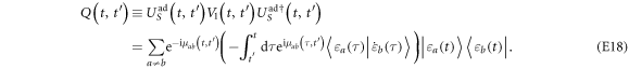
  is evolving in time since it corresponds to differences of the instantaneous energy eigenvalues, but we suppress the time dependence for notational brevity. We show in appendix G how, by performing a transformation back to the Schrödinger picture, along with a double-sided adiabatic approximation, we arrive from equation (53) at the Schrödinger picture adiabatic master equation in Lindblad form:

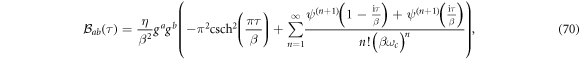
where the Hermitian Lamb shift term is

and we have defined

5. An illustrative example: transverse field Ising chain coupled to a boson bath
5.2. Correlation function analysis
Appendix B. Markov approximation bound.
Following the notation in this section, the expression for  should not include a g2, and equation (B8) should read:

Appendix E. Non-adiabatic corrections.
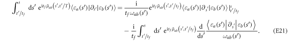
Equation (E18) should read
Equation (E19) should read:

Equation (E20) should read:

equation (E21) should read
Equation (E22) should read:

Appendix F. Short time bound.
We provide the following rewrite of this appendix section that includes numerous fixes.
We wish to bound the error associated with neglecting Θ in equation (40), i.e., we wish to bound

Using that the operator  satisfies:

we can write a formal solution for  as:
as:

Therefore we can bound:


where we used equation (E17) and the fact that supoperator norm between two unitaries is always upper bounded by 2 in the second line, and the standard adiabatic estimate to bound  (recall subsection E.2). While h of equation (26) is expressed in terms of a matrix element, a more careful analysis (e.g., [10]) would replace this with an operator norm. Thus we shall make the plausible assumption that
 ![$h\sim {t}_{f}{\mathrm{max}}_{{t}^{\prime }\in [t-\tau ,t]}\parallel {\partial }_{{t}^{\prime }}{H}_{S}({t}^{\prime }){\parallel }_{\infty },$](https://content.cld.iop.org/journals/1367-2630/17/12/129501/revision1/njp521699ieqn11.gif) and, dropping the subdominant
and, dropping the subdominant  we can write

where ![$\tilde{h}={\mathrm{max}}_{{t}^{\prime }\in [t-\tau ,t]}\frac{{t}_{f}}{{t}^{\prime }}\parallel \left[{H}_{S}(t)-{{\rm{e}}}^{-{\rm{i}}{H}_{S}(t){t}^{\prime }}{H}_{S}(t-{t}^{\prime }){{\rm{e}}}^{{\rm{i}}{H}_{S}(t){t}^{\prime }}\right]{\parallel }_{\infty }.$](https://content.cld.iop.org/journals/1367-2630/17/12/129501/revision1/njp521699ieqn13.gif) We can now bound the error term in equation (42b). Let
We can now bound the error term in equation (42b). Let 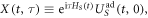 so that
  We can then write
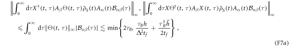
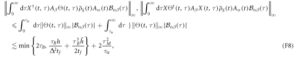


The first term on the rhs of (F6a) is the approximation we have used in equation (42b). The terms in (F6b) and (F6c) can be bounded as follows, using equation (F5), the unitarity of X, the fact that  and recalling that
  First we assume that equation (12) applies. Then:
where in the last inequality we used the fact that if  then
then ![${[\mathrm{min}(2,x)]}^{2}={x}^{2}\leqslant 2x,$](https://content.cld.iop.org/journals/1367-2630/17/12/129501/revision1/njp521699ieqn19.gif) and if
and if  then again
 ![${[\mathrm{min}(2,x)]}^{2}=2\mathrm{min}(2,x)\leqslant 2x,$](https://content.cld.iop.org/journals/1367-2630/17/12/129501/revision1/njp521699ieqn21.gif) with
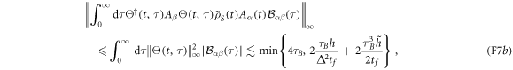
with  in order to avoid having to extend equation (12) to higher values of n. In all, then, the approximation error in equation (42b) is
 ![$O[\mathrm{min}\{{\tau }_{B},\frac{{\tau }_{B}h}{{{\rm{\Delta }}}^{2}{t}_{f}}+\frac{{\tau }_{B}^{3}\tilde{h}}{{t}_{f}}\}].$](https://content.cld.iop.org/journals/1367-2630/17/12/129501/revision1/njp521699ieqn23.gif)
Next we recall from the discussion in section 2.3 that equation (12) must, in the case of a Markovian bath with a finite cutoff, be replaced by the weaker condition (23), reflecting fast decay up to  followed by power-law decay. In this case the terms in (F6b) can instead be bounded as follows:
in place of (F7b). A similar modification can be computed for the term in (F6c). To compute the order of  we recall that
  (equation (75)), and that
  Thus
Thus ![$\frac{{\tau }_{M}^{2}}{{\tau }_{\mathrm{tr}}}\sim {[{\omega }_{c}\mathrm{ln}(\beta {\omega }_{c})]}^{-1}.$](https://content.cld.iop.org/journals/1367-2630/17/12/129501/revision1/njp521699ieqn28.gif) It follows that we can safely ignore the
It follows that we can safely ignore the  term in equation (F8) provided equation (77) is satisfied. The analysis of the term in (F6c) does not change this conclusion.