


Abstract
An important challenge in quantum science is to fully understand the efficiency of energy flow in networks. Here we present a simple and intuitive explanation for the intriguing observation that optimally efficient networks are not purely quantum, but are assisted by some interaction with a 'noisy' classical environment. By considering the system's dynamics in both the site-basis and the momentum-basis, we show that the effect of classical noise is to sustain a broad momentum distribution, countering the depletion of high mobility terms which occurs as energy exits from the network. This picture suggests that the optimal level of classical noise is reciprocally related to the linear dimension of the lattice; our numerical simulations verify this prediction to high accuracy for regular 1D and 2D networks over a range of sizes up to thousands of sites. This insight leads to the discovery that dramatic further improvements in performance occur when a driving field targets noise at the low mobility components. The simulation code which we wrote for this study has been made openly available at figshare4.
Export citation and abstract BibTeX RIS

Content from this work may be used under the terms of the Creative Commons Attribution 3.0 licence. Any further distribution of this work must maintain attribution to the author(s) and the title of the work, journal citation and DOI.
The study of energy transfer in quantum networks is a broad field, ranging from abstract theoretical studies [1–11] through to experimentally observed transport dynamics of real networks [12, 13], for instance in light-harvesting complexes [14–20]. An important observation is that while generally a purely quantum mechanical energy transfer process (i.e. a quantum random walk) is inherently faster than the classical equivalent, nevertheless when one measures the efficiency of a network in terms of the time needed for a unit of energy to completely traverse it, then it is often optimal to temper the purely quantum dynamics with a degree of classical 'noise'. This noise may be, for example, dephasing of the quantum state [21] or a spontaneous hopping process; in each case the ideal level of noise is non-zero, and for the latter case this has recently been verified for networks of arbitrary topology and sizes up to thousands of sites [22].
It is well established that the optimal level of noise varies dramatically according to the particular features of the underlying system. For example, for an input and an exit site bridged by a topologically disordered network, noise leads to classical diffusion, and this limit has been found to be generally optimal [23]. A similar geometrical setup finds that noise generally improves systems with low efficiency and deteriorates those specific instances which perform particularly well under quantum diffusion [24, 25]. Further, it is well known that for homogeneous linear chains where the excitation enters on one end and exits on the opposite end, any noise at all is detrimental [22, 26–30]. Intriguingly, however, with the exception of some specific cases such as the preceding one, noise generally remains advantageous.
In traditional Förster theory [31] dephasing noise assumes a beneficial role by inducing line-broading, which improves the transfer rate between sites with energy mismatch. At the same time, it renders the resulting dynamics incoherent, and hence suboptimal. By contrast, the early work of Haken, Strobl and Reineker [32–34] considers both classical and quantum diffusion as contributing to transport, and in some limits even captures the fact that a certain amount of noise can be advantageous [27, 35]. However, it does not provide a deeper insight into this intriguing observation and the subtle effects giving rise to it.
Therefore, various explanations for classically-assisted quantum transport have recently been proposed [26, 27, 35–45] (see [46] for a review of earlier works on quantum transport phenomena). For example, [27] addresses both line-broadening and the suppression of destructive interference as basic mechanisms underlying this phenomenon. Very recently, [47] introduced several further mechanisms occurring in simple energy-transfer models with few sites, which may also persist in larger networks, whereas [48] provides a simple way of understanding why there exists an optimal amount of exciton wavefunction delocalisation in photosynthetic networks in terms of a 'quantum Goldilocks principle'. Generally, in networks with disorder (e.g. irregularities in the site couplings) the quantum state can become locally trapped [3]. Injecting classical noise can break this localisation, as has for instance been recently experimentally observed in ultra-cold atomic systems on optical lattices [49]. Similar to classical noise, even a very weak local measurement can suppress Anderson localization, hence enhancing quantum transport [50]. Classical noise has been found to be advantageous even in perfectly ordered networks. For such systems it is generally argued that quantum networks suffer from a kind of locking effect, where destructive interference occurs between the different possible pathways to the exit site.
Following the notion of invariant subspaces introduced in [27], an equivalent statement of this effect is that some of the spatial eigenstates of the system (which are in general highly non-local) may have zero amplitude on a given site—if such a site happened to be the exit, then any part of the initial wavefunction associated with such an eigenstate would never be able to leave the network. Classical noise disrupts such eigenstates, thus alleviating the problem. This concept has recently also been labelled the 'orthogonal subspace' to the trapping superoperator and used to derive an asymptotic scaling theory for energy transport [51]. In this paper we will say that a system exhibits 'quantum locking' if there is a finite probability of energy remaining on the network as  (for zero noise). Strict quantum locking occurs in certain network topologies, however, a much larger class of networks exhibits an 'approximate' variant of it, where the amplitude of certain eigenstates on the exit site is small (as opposed to identically zero), i.e. there is a degree of destructive interference present, however, without effecting a complete cancellation of the wavefunction on the exit site. As we have defined it above, quantum locking is perhaps the most intuitive way in which destructive interference may inhibit transfer to the exit site. However, note that interference-related effects can also have other consequences affecting transport, and the mechanism we discuss in this paper could alternatively be seen as an instance in this category.
It is well-established that quantum locking, despite its importance and conceptual elegance, does not provide a comprehensive explanation for noise-assisted quantum transport even in highly ordered networks: there are a number of basic cases where classical noise does assist quantum transport, and yet provably there is no quantum locking effect present. The simplest example (figure 1(a)) is the one-dimensional (1D) chain with an exit site at one end and an initial excitation site within the chain [22, 30]. Indeed, a deformed linear chain constitutes an example without even approximate quantum locking, and yet classical noise remains beneficial (see appendix
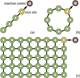
Figure 1. Some of the regular network topologies considered here: (a) linear (b) ring, and (c) rectangular lattices. Each circle represents a site, i.e. a molecule or other entity which can be excited by a quantum of energy; the excitation can hop from one molecule to the nearest neighbouring molecule and leave the network via the exit site.
Download figure:
Standard image High-resolution imageIn this paper, we will argue that classically-assisted quantum transport in regular networks can be intuitively understood by viewing the dynamics through a combination of the site-basis and the momentum-basis pictures. We begin by explaining the basic principle, before developing the idea more formally and finally checking the predictions versus intensive numerical simulations. Our analysis in this paper is restricted to the case where there is a single quantum of energy in the network, although we anticipate that our argument translates straightforwardly to multiple energy quanta, as long as the density of excitations is low and interactions between excitations rarely happen. (We note in passing that in certain photosynthetic systems, the single excitation model is certainly appropriate since fewer than 10 photons are absorbed per molecule per second [52], while the coupling strength of molecules  , and thus the transport process is
  times faster than the absorption process.) We identify the site basis with states written as
  , which corresponds to the energy being definitely located at site-i, and we will assign the index x to the 'exit' site. We will presently define the momentum basis as the standard canonical complement to the site basis.
To explain the process let us first consider a rather contrived model for classical noise: we will subject our quantum system to a periodic series of instantaneous events where the state is completely dephased in the site basis. We initialise our system by injecting energy at some randomly chosen location, i.e. we select some random initial state  , and there follows a period of evolution before the first dephasing event. State
  will of course correspond to a broad superposition of states in the momentum picture. The components with a high group velocity will rapidly transit the network and will be the first to impinge on the exit site (to 'hit' that site in the terminology of random walks). There will then be a finite probability per unit time of the energy exciting the system; over time if the energy does not exit, the wavefunction will skew further and further toward lower group velocity terms. Suppose that this has occurred for some period, and then the first of our classical noise events occurs.
This dephasing event is equivalent to measuring the system in the site basis, and then forgetting the outcome. In effect we are reinitialising the system to some state  (although of course this choice is not purely random, since a given site j is more likely if it is closer to the original site i). But regardless of which
  we select, the important point is that the momentum distribution is now once again broad and includes elements with a high group velocity. Thus our periodic classical noise process repeatedly reinvigorates, or rejuvenates, the momentum distribution and so counters the skew towards low mobility elements. In-between noise events the high group velocity components will reach the exit and be removed. Clearly there is some optimal rate of classical noise: if it is too strong, i.e. the frequency of the events is too high, then after one event another will occur before the more rapidly propagating components can exit—this would merely reduce the quantum random walk to a classical one without any advantage. Conversely, too weak a level of classical noise will mean that we miss the opportunity to rejuvenate the momentum distribution.
This line of thought leads one to conclude that the optimal frequency of the classical noise should depend on the lattice size. In a larger lattice, the high momentum components have further to go to reach the exit, and so a longer period should be allowed between the classical noise events. One might expect a  dependence, where N is the linear dimension of the lattice (so that a square lattice has N2 sites). In the following, this conjecture is verified to a high degree of accuracy by our numerical simulations.
The transport of energy in a regular network with identical sites can be modelled as ( )
)

where the coherent transport is given by the Hamiltonian

where h.c. denotes the Hermitian conjugate and the noisy classical process is either classical hopping (CH)

with

or pure dephasing (PD)

and the excitation leaves the network via the exit site-x according to the process

Here, ρ is the state of the network,  and
and  are ladder operators describing transitions between the ground state
  and the excited state
  of the site-i,
  denotes two connected sites, J is the coupling strength,
  and p are the relative weightings of the quantum and classical processes (
 ) [22, 23, 53], the constant
  for 1D chain, 2D square, and three-dimensional (3D) cubic lattices, respectively, and Γ is the strength of the exit coupling from the network. Note that we do not need to explicitly include the reaction centres depicted in figure 1 in our model.
Our single-excitation subspace is spanned by  , where the state
  and
and  denotes the overall ground state of the entire system. When p = 0, the transport process is purely quantum mechanical; when p = 1, the transport becomes a completely classical random walk in the CH model, and will be switched off entirely in the PD model. Here our analysis will be largely focused on the CH model, but we note that the same basic argument will apply to PD.
In order to measure the transport efficiency, we look at the probability that at time t the energy quantum has failed to exit the network, ![$P(t)={\rm Tr}[\rho (t)\sum _{i=1}^{N}\sigma _{i}^{+}\sigma _{i}^{-}]$](https://content.cld.iop.org/journals/1367-2630/17/1/013057/revision1/njp507415ieqn22.gif) . This is the 'population' remaining on the network. In cases where there is no quantum locking all population eventually vanishes; one such system is the 1D chain with the exit at one end of the chain, as shown in figures 1(a) and 2(a). Moreover, it will always vanish when we have finite classical noise. Therefore we can gauge the transport efficiency, or rather the inefficiency, by finding the average dwelling time in the network which we define as
. This is the 'population' remaining on the network. In cases where there is no quantum locking all population eventually vanishes; one such system is the 1D chain with the exit at one end of the chain, as shown in figures 1(a) and 2(a). Moreover, it will always vanish when we have finite classical noise. Therefore we can gauge the transport efficiency, or rather the inefficiency, by finding the average dwelling time in the network which we define as  . We regard a network as optimised when this quantity has been minimised.
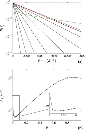
Figure 2. For a 1D chain of N = 40 sites with an 'exit' site at one end (see figure 1(a)), and a range of classical hopping rates p, we plot (a) the probability P(t) that the energy quantum is still on the network, and (b) the average dwelling time  . The energy is initially located at a randomly chosen site, so that curves are computed using an initial
  . We set the exit coupling to be
  . In (a), the green line corresponds to the pure coherent transport case p = 0, the red line corresponds to the pure CH case p = 1, and black lines represents
  from bottom to top, respectively. In (b), one can find that the average dwelling time is minimised at a finite CH rate
  .
.
Download figure:
Standard image High-resolution imageFor the 1D chain, the average dwelling time for different CH rates p is shown in figure 2(b). We note that the average dwelling time is minimized at  for the chain with lattice size N = 40 when we take the exit to be site N.
In the single-excitation subspace of the 1D chain, the momentum eigenstate with wave vector  is
is

where  ,
,  , and a is the lattice constant. The eigenenergy of the state
  is
is  , and the corresponding group velocity is
  . Therefore, a wavefunction formed from states in the middle of the band has a high group velocity
  , while a superposition of states at the edge of the band has a low group velocity
  .
.
Suppose that at t = 0 our excitation is at site i, then inverting equation (7) we see that in the momentum basis the state has a probability of  associated with the eigenstate
  . Hence, the site-localised excitation will have significant population in both the high- and the low-velocity states. As we have discussed, the higher-velocity components leave the system first, leaving behind an ever more slowly falling population remnant.
Suppose that a finite level of CH is present. Even though our noise models (equations (3) and (5)) are continuous, we can map this onto discrete events whereby the excitation is effectively reinitialized during the transport process. For a short time  , the state evolves as

In the single-excitation subspace, the effect of CH can be expressed as

where


Hence, a CH event  corresponds to a measurement of the position of the excitation at site j followed by moving the excitation to a randomly chosen neighbouring molecule i, i.e. effectively reinitialising the excitation to one of the neighbouring sites.
The presence of dephasing PD will have essentially the same effect, of course without the final 'hop'; it can be expressed as

where


Thus for both our models of continuous classical noise, we may equivalently think in terms of an occasional reinitialisation process where part of the population in low-velocity states will be promoted to high-velocity states. To optimize the transport efficiency, the high-velocity component has to leave the network before the next CH or PD event happens. Therefore, the optimal level of classical noise p decreases with the time required to leave the network, i.e. the lattice size. Notice that this implies that in the limit  , the optimal rate
  . In other words, for very large ordered lattices we expect that the classical noise mechanism described here will no longer be advantageous.
In figure 3 we show how the momentum distribution  evolves over time, starting from a broad initial distribution corresponding to a site eigenstate
  . For the purely quantum limit p = 0 one finds that populations in high-velocity states,
  , vanish much faster than those in low-velocity states, so our initially even distribution becomes highly skewed as time passes. For the pure CH case, populations with different momenta vanish with almost the same rate, but this rate is much slower than the coherent transport (note the units of the time axis are ten times greater). In the 'best of both worlds' case a modest level of CH serves to rejuvenate the distribution, i.e. to keep it relatively even. The high-velocity components can still escape from the network quite efficiently, while at the same time the lingering wings of the distribution are depleted as we transfer population from low-velocity states to high-velocity states via CH events. As a result, although population in high-velocity states persists for longer than it does in the purely quantum case, nevertheless the overall transport efficiency is increased. This explanation remains valid in the presence of moderate levels of disorder as we show in appendix

Figure 3. Colour maps showing the populations associated with momentum eigenstates Pk on the one-dimensional chain lattice with N = 40 sites (see figure 2) for (a) the pure coherent transport case p = 0, (b) the optimal CH rate p = 0.029, and (c) the pure CH case p = 1. Note that the time range (horizontal axis) is ten times greater for (c), and that therefore the pure classical hopping is very inferior to the other two. Inset plots show population distributions at the time  , with total probability stated.
Download figure:
Standard image High-resolution imageThe analysis so far has been presented in terms of the 1D lattice, but the same arguments equally apply to higher dimensional regular lattices. We now present the results of numerical simulations which we have performed on 1D, 2D and 3D arrays. In all cases we observe a  scaling of the optimal noise level, where N is the linear dimension of the array. This is fully consistent with the expectation that the phenomenon of momentum rejuvenation applies to regular networks of any dimension.
To be specific, we should in fact anticipate that the quantity  will scale in this way, according to the following reasoning: the effective rate at which we reinitialise the momentum distribution goes with pJ, but the rate at which the quantum coherent evolution occurs is proportional to
  , see equation (2). Thus the width which the excitation's spatial distribution can reach between reinitialisation events varies with
  , and we expect that this width should be proportional to the linear lattice size N (and therefore the average distance between a randomly chosen site and the exit site). Thus we expect to see

where b is a constant of proportionality and we have also added an adjustment c to allow for finite size effects (which should be significant only for small arrays). We do not predict the specific values of these constants, which will depend for example on the location of the exit site (corner, edge or internal to the lattice). However, we expect that the above expression will be accurately obeyed if b and c are treated as free fitting parameters. In figure 4 we display the results of a series of numerical experiments where we test our hypothesis. We find that the proposed function does indeed fit the data well. Corresponding fitting parameters and confidence intervals are shown in appendix
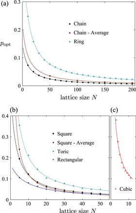
Figure 4. The optimal classical hopping (CH) rate  of (a) one-dimensional chain lattices and ring lattices with N sites, (b) two-dimensional square lattices, torus lattices with N × N sites, and rectangle lattices with
  sites, and (c) three-dimensional cubic lattices with
  sites. The optimal CH rate depends on the position of the exit site. The exit site is placed at the end on chain lattices and a corner on square, rectangular, and cubic lattices as examples. Optimal CH rates given by the average remaining population for all possible positions of the exit site are also considered for chain and square lattices. The curves are obtained by fitting the function
  , and fitting parameters are shown in table C.1. We have supposed that
  and the energy is initially located at a randomly chosen site.
Download figure:
Standard image High-resolution imageTable C.1. Fitting parameters of curves in figure 4.
| Lattice type | b | c |
|---|---|---|
| Chain | 1.453 | 8.311 |
| Chain—average | 2.081 | 7.371 |
| Ring | 4.483 | 3.657 |
| Square | 1.493 | 1.128 |
| Square—average | 1.209 | −1.17 |
| Toric | 2.404 | −0.660 |
| Rectangular | 1.443 | 7.068 |
| Cubic | 1.29 | −0.4443 |
It is worth noting that one can obtain a reasonable estimate of the optimal rate of classical noise merely by applying our simple discretised picture: fully dephasing events occur intermittently, in place of the real continuous noise. We suppose that the single-excitation state evolves coherently, i.e. p = 0, and is completely reinitialized with the period τ. A complete reinitialization reads

which means the excitation is initialized at a randomly chosen site. If P(t) denotes the population in the network at time t when p = 0 (i.e. the green curve in figure 2), the population after n occurrences of the reinitialization event with period τ is  . Therefore, roughly speaking, the population in the network decays with a rate
  . For the chain with the size N = 40 shown in figure 2, we extract a maximum of the decay rate
  at
at  . Comparing the frequency of complete reinitializations with the CH rate,
  , then this optimal period corresponds to the CH rate p = 0.023, which is remarkably close to the observed optimal CH rate p = 0.029.
How does the role of noise in overcoming quantum locking compare to its role in this momentum rejuvenation picture? We know that quantum locking is a significant effect in many systems. For example in a regular 2D square array there will always be finite quantum locking in the absence of noise, and therefore the assistance provided by noise is, in part, to remove this locking effect. However there are also many cases where there is no quantum locking in the zero-noise limit. Our numerical simulations indicate that such cases include the following (for any location of the initial state and exit, unless otherwise noted):
- A 1D array with the exit at one end, and the initial excitation site within the chain.
- A 2D array
 with and the exit in a corner.
 - Any 2D array with dimensions , where N* and M* are two different primes.
- Any 2D array with multiple exit sites forming the perimeter (shown analytically in appendix
D ). - Any 2D array with (arbitrarily small) random perturbations to the coupling strengths or the on-site energies.


For all these cases we would expect that the momentum rejuvenation picture still applies, since it has no special reliance on symmetries in the system. And indeed in all these cases we find that there is a finite value of classical noise which optimises the network. Therefore we conjecture that the momentum rejuvenation picture is a complementary explanation for noise-assisted transport in regular arrays; which not only captures the important role of noise in disrupting quantum locking, but also applies to networks which do not feature locking.
In support of this view, we note that figure 4(b) contains one instance of a network where locking is present (the square array) and one for which it is not (rectangular with exit on the corner). For small networks we note that the optimal amount of noise is higher for the square lattice compared to the rectangular one. In fact, this is not unexpected since here the noise is advantageous for overcoming the locking effect as well as maintaining a broad momentum distribution.
One might ask if the random classical noise from a network's environment is an ideal means of maximising the transport efficiency, or whether other mechanisms might lead to even higher efficiency. According to the picture we have presented, classical noise effectively rejuvenates the whole momentum distribution indiscriminately. It would presumably be even more beneficial if one could somehow preferentially rejuvenate the low velocity states, leaving the high velocity state unperturbed. We now present a simple one-dimensional example where this becomes possible when a global driving field is applied.
Let us assume that each lattice site possesses an additional excited state  (see figure 5(a)). These higher excited levels form a second excited tier of the network, which will in general experience different hopping strengths
  . For simplicity let us assume for now that no classical noise is present and that the coupling strength
  is negligible compared to J. (Note that only
  is a requirement for the control protocol described here, but the present assumption makes the following argument particularly straightforward.) As a result, we have purely quantum transport in the lower excited manifold spanned by the
  levels, governed by the hamiltonian 2 with p = 0.

Figure 5. (a) Level structure of molecules with driven transitions between the excited state  and the higher excited state
  . Because of the hopping coupling, a 'conduction' band with the width
  is formed around the energy of the state
  . (b) Colour map showing the populations associated with momentum eigenstates Pk on a network with driving fields; as in figure 3 (which shares the same colour scale), a one-dimensional chain lattice with N = 40 sites is considered as an example. Here, the Rabi frequency
  and the decay rate
  . Comparison with figure 3 shows that the population remaining on the network at time
  is significantly smaller than for the passive optimal quantum-classical hybrid network (0.0024 versus 0.0473).
Download figure:
Standard image High-resolution imageLet ω be the energy difference between  and
and  ; the application of global driving fields with frequencies
  will then drive transitions between low velocity
  states (indicated by red circles in figure 5(a)) and
  states. At the same time, high-velocity transitions are detuned and thus suppressed. The driving Hamiltonian is given by

where the Rabi frequency Ω is proportional to the intensity of the applied field, and  and
and  are ladder operators describing transitions between the state
  and the state
  of the site i.
The only other process we require is dissipative relaxation from the second excited tier back into the lower excited manifold, e.g. phonon-assisted transitions which randomise the momentum of the electronic state. These can be described by the following Lindblad superoperator

where γ is the decay rate from the state  to the state
  .
.
Under these circumstances, the population is preferentially pumped from low-velocity states to the excited state, from which it decays to any momentum state (as shown in figure 5(b)). Thus by targeting the low-velocity state we achieve a much faster transfer (i.e. lower population remaining on the network) than for the optimal quantum-classical hybrid network shown in figure 3(b).
In conclusion, we offer an intuitive explanation for the observation that classically assisted quantum transport can be more efficient than pure quantum evolution, even in systems where quantum locking is negligible. We predict that the optimal level of classical noise will scale inversely with the linear dimension of the array, and our numerical simulations have confirmed this behaviour for systems of up to 2500 sites. The picture we have presented is one in which the classical environment acts to continually rejuvenate the momentum distribution of the quantum particle as it traverses the network. In general terms the existence of wave packet components with low velocity can classed as an interference effect; here we have introduced a momentum picture which we believe provides the correct intuitive perspective for understanding this aspect of noise-assisted quantum transport. We use the intuition gained from adopting this viewpoint to show that the use of global driving fields can be far more efficient than simple random noise.
4http://figshare.com/articles/Quantum_Classical_Hybrid_Transport_Simulations/10501058
Acknowledgments
We thank Viv Kendon and Shane Mansfield for helpful conversations. This work was supported by the EPSRC platform Grant 'Molecular Quantum Devices' (EP/J015067/1) and by the National Research Foundation and Ministry of Education, Singapore. The authors gratefully acknowledge financial support from the Oxford Martin School Programme on Bio-Inspired Quantum Technologies. The work of FC has been supported by EU FP7 Marie-Curie Programme (Career Integration Grant) and by MIUR-FIRB grant (Project No. RBFR10M3SB).
Appendix A.: Deformed chains
In this appendix we discuss an example of the momentum rejuvenation mechanism for a system where there is not even approximate quantum locking.
In uniform chains with the 'exit' site at one end, all eigenstates have finite amplitudes on the exit site given by  for the eigenstate
  . Hence, there is no strict quantum locking in these uniform chains (
 ). However, in such a chain all states with a k close to 0 or π are only very weakly coupled to the exit site, whilst those with
  have maximal coupling. These weakly coupled states may then cause an approximate quantum locking effect. Let us now instead consider a deformed chain with N sites and the 'exit' site at one of the ends, for which the Hamiltonian reads

where  and
and  . In this deformed chain, the eigenstates are given by

where  ;
;  ;
;  ,
,  ;
;  and
and  . The eigenenergy of the state
  is
is  . For the amplitude of the state
  on the exit site one finds
  if
if  and
and  if
if  . Therefore, all eigenstates are equally coupled to the exit site except two of them (
 ) whose coupling is reduced by only a factor of
  .
.
It is then fair to state that there is no significant level of quantum locking preventing transport to the exit site, so that from the quantum locking picture one would not expect noise to be advantageous. By contrast, considering the momentum space distribution of the chain, we expect that momentum rejuvenation still ought to play a beneficial role. Our numerical results shown in figure A1 confirm that the concept of noise-assisted transport remains fully applicable. In this case this is clearly due to the momentum rejuvenation effect, rather than quantum locking.
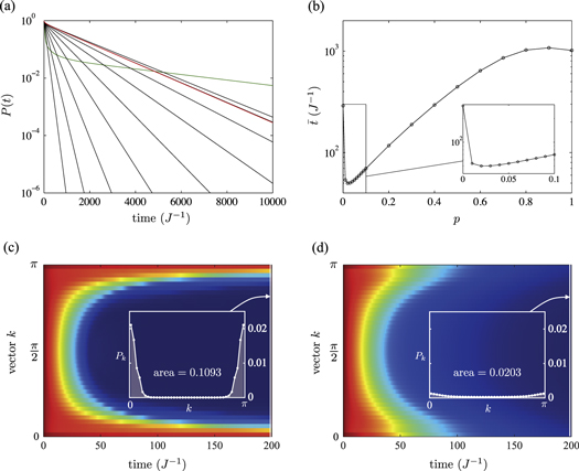
Figure A1. Energy transport in deformed 1D chains of N = 40 sites with an 'exit' site at one end. The rates of classical hopping are scaled according to the quantum hopping rates. (c) and (d) share the same colour scale with figure 3.
Download figure:
Standard image High-resolution imageAppendix B.: Disorder
The momentum rejuvenation mechanism is robust to disorder as shown in figure B1 . In the presence of disorder, pure quantum transport is slowed down by wave-function localisation [3, 39, 40, 48]. However, as long as there is no energy eigenstate that is completely decoupled from the exit site, the excitation can still eventually leave the network to the reaction centre. When disorder is not too strong and the momentum eigenstates are still a good approximation of the energy eigenstates (as is, e.g., the case for the 10% fluctuations in the quantum hopping strength underlying figure B1), the picture of momentum rejuvenation enabling faster transport remains valid. Generally speaking, disordered systems then benefit from noise both for overcoming localisation as well as for momentum rejuvenation. As long as the level of disorder is weak, momentum rejuvenation continues to play the more important role in noise-assisted quantum transport.
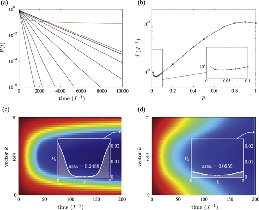
Figure B1. Energy transport in disordered 1D chains of N = 40 sites with an 'exit' site at one end. In these disordered chains, the quantum hopping strength is normally distributed with the average value  and variance
  . The populations P(t) and Pk (thereby
  ) are the average values obtained from 1000 samples. Comparing (a) and (b) with figure 2, the energy transport is generally slowed down by the localisation effect. An optimal CH rate still exists in (b). As shown in (c) and (d) (which share the same colour scale with figure 3), the momentum rejuvenation is still significant in these disordered chains.
Download figure:
Standard image High-resolution imageAppendix C.: Fitting parameters
The parameters used in the line fittings for figure 4 are shown in table C.1. In table C.2 , we show the 95% confidence interval of the fitting parameters for figure 4, which were obtained by the MATLAB function 'fit'.
Table C.2. 95% confidence bounds of fittings in figure 4.
| Lattice type | b | c |
|---|---|---|
| Chain | (1.429, 1.477) | (7.892, 8.731) |
| Chain—average | (2.041, 2.12) | (6.093, 8.649) |
| Ring | (4.435, 4.531) | (3.441, 3.873) |
| Square | (1.439, 1.547) | (0.8296, 1.426) |
| Square—average | (1.178, 1.239) | (−1.292, −1.049) |
| Toric | (2.286, 2.523) | (−0.969, −0.352) |
| Rectangular | (1.344, 1.541) | (5.937, 8.200) |
| Cubic | (1.071, 1.51) | (−0.8898, 0.001 22) |
Appendix D.: Perimeter exit
For a rectangular network of the type shown in figure D1 , the Hamiltonian reads

Here, the on-site energy  and quantum hopping strength
  need not be all identical, but we assume that
  for all nearest neighbour terms. If all sites on the perimeter are exit sites (yellow sites in figure D1), i.e. coupled to the reaction centre, a locked state is an eigenstate of the Hamiltonian with zero amplitude on the whole perimeter. In general, in the single-excitation subspace the locked state can be written as

where the amplitude  for all
  . Here, the set
  contains the four corner sites, and the set
  contains all other sites on the perimeter. Furthermore, we use
  to denote sites on an imagined inner perimeter (blue sites in figure D1), all of these are coupled to perimeter sites. Since,
  is an eigenstate,
  where
where  is the eigenenergy of the locked state. For perimeter sites in
  ,
,  , where the site
  is the only off-perimeter site coupled to the perimeter site-i. However, from
  and
and  it follows that
  .
.

Figure D1. A rectangular network with the whole perimeter filled by exit sites.
Download figure:
Standard image High-resolution image
Therefore, for a state to be locked, not only does its amplitude on the perimeter have to be zero, its amplitude on the inner perimeter must also vanish. Letting the inner perimeter now take the role of the exit sites and repeating the previous discussion, one finds by induction that a locked state possesses zero amplitude on the whole network. In other words, there is no locked state for such a network with the whole perimeter filled by exit sites.