


Abstract
We write the charge-free Maxwell equations in a form analogous to that of the Dirac equation for a free electron. This allows us to apply to light some of the ideas developed for the relativistic theory of the electron. Valuable insight is gained, thereby, into the forms of the optical spin and orbital angular momenta.
Export citation and abstract BibTeX RIS

Content from this work may be used under the terms of the Creative Commons Attribution 3.0 licence. Any further distribution of this work must maintain attribution to the author(s) and the title of the work, journal citation and DOI.
1. Historical introduction
Maxwellʼs equations are remarkable in that they have survived the introduction of quantum theory and of both the special and general theories of relativity. The form in which the equations are expressed has changed many times, however. It is interesting to note that in his original paper, Maxwell used no fewer than twenty symbols to represent his various fields [1]. It was Heaviside who, in the words of Sir Edmund Whittaker, 'clear(ed) away this accumulation of rubbish' and gave us Maxwellʼs equations in their now familiar form [2]. For the free electromagnetic field, that is in the absence of charges and currents, we write these as
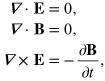

Here we have used the natural system of units in which ε0 and μ0 are both unity, as is the speed of light. The quantities  and
and  are the (real) electric field and the magnetic field (or perhaps, more properly, the magnetic flux density). It is common, also, to write these in a manifestly Lorentz-invariant form by use of the field tensor
  or, indeed, in general covariant form to allow for the description of non-inertial frames of motion or the effects of a gravitational field [3, 4].
We shall be interested in the links between Maxwellʼs equations and those arising in quantum mechanics and especially in relativistic quantum theory. Perhaps the first step in this direction was published in the earliest days of the old quantum theory, although such a link was not the initial aim. Riemann and Silberstein introduced the complex vector field

the effect of which is to reduce Heavisideʼs four equations into just two [5–8]
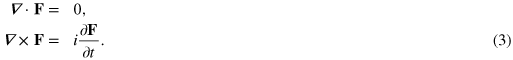
The Riemann–Silberstein vector appears in some textbooks [9, 10] and has been applied to a variety of problems in classical electromagnetism including calculating the fields associated with a moving charge [11]. Of these two equations, the first may be viewed as a constraint on the forms of the allowed Riemann–Silberstein vectors with the second providing the dynamics. We can write the second equation in a matrix form [12–16]

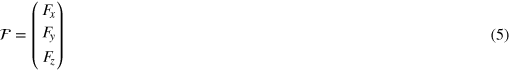
where  is the column vector
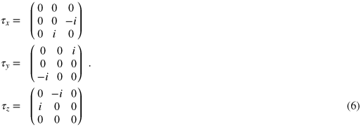
and τ is a vector, the components of which are the familiar spin-1 matrices [17]
When written in the form (4) Maxwellʼs equations are reminiscent of the Schrödinger and Dirac equations. This is yet more apparent if we multiply by ℏ and introduce the momentum operator, 

and identify  as our Hamiltonian. It is interesting to note the similarity between this equation and the two component theory of Weyl, appropriate for neutrinos, which we can obtain by replacing the three-component
  with a two-component field and the spin-1 τ-matrices with the familiar Pauli matrices appropriate for spin-
 particles [18].
Although it is not our main aim, no account of this topic would be complete without a discussion of the photon wave function. It is not surprising, given the above analysis, that many authors have sought a wave function for the photon. Perhaps the most natural approach is to adopt the Riemann–Silberstein vector, or equivalently  , for this purpose [12, 13, 15, 16, 19–21]. One objection we might raise to this is that
  has the dimensions of the square root of an energy density rather than the square root of a (probability) density normally associated with a wave function. It has been suggested that we can solve this problem by dividing
  by
by  or
or  so that each frequency component of the field is divided by
  [22–26]. The problem with this, however, is that the resulting wave functions exhibit highly nonlocal behaviour and a number of other undesirable features [16]. We can take the Riemann–Silberstein vector as our wave function but it is necessary to get the dimensions right either by dividing by the mean energy or by introducing the reciprocal of the Hamiltonian into the definition of our scalar product. These issues are discussed further in the excellent review article by Białynicki-Birula [16].
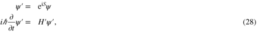
It is not our main aim to investigate quantum optical effects and we neither require nor seek a photon wave function. Instead, we seek to exploit the analogy between Maxwellʼs equations and the Dirac equation to learn something about, classical optics and, in particular, the mechanical properties of light. There exist a variety of Dirac-like formulations of Maxwellʼs equations, but the most appropriate for our purposes is essentially that proposed by Darwin [27, 28] for a six-component 'spinor'1 ψ:
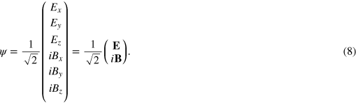
Our time-dependent Maxwell equations then acquire the form

where each element in the matrix represents a 3 × 3 matrix. It is this equation that we shall refer to as the optical Dirac equation. It is important to state this clearly as there are a number of equations that could also justifiably be given this title; in addition to those already mentioned earlier, for example, we should also mention in this regard the existence of Dirac-like formulations of Maxwellʼs equations based on four-component spinors [32, 33].
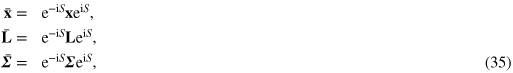
We should note that our spinor (8) is not unique. We shall find the physically relevant mechanical properties of the fields are expressed in terms of products of ψ and its conjugate  and so we can multiply ψ by any phase factor and leave the physical properties unchanged. This is analogous, of course, to the undefined global phase of the wavefunction in quantum mechanics. There is also a more subtle symmetry between the electric and magnetic fields, due to Heaviside and Larmor [34–36]. This is the observation that the free-field Maxwell equations (1) are invariant under the transformation

where θ is any angle. It follows that physically meaningful properties of the field should also respect this symmetry [37] and this idea has been useful in deriving forms for the spin and orbital angular momenta of the field [38, 39] and for its helicity [40–45]. We note that a variant of this symmetry applies also for gravitational waves and leads to locally conserved quantities analogous to those for electromagnetic waves [46]. We can enact the transformation (10) on our spinor by means of a unitary operator in the form

and it follows that, any spinor of this form will give equivalent results. The choice of spinor is, therefore, a conventional one and we opt to work with ψ as given in (8).
In this paper we apply to our optical Dirac equation some of the methods that have been developed for Diracʼs electron equation. We find, in particular, that the Foldy–Wouthysen transformation and the elimination of optical, Zitterbewegung lead, in a natural way, to familiar slowly-varying quantities.
The paper is intended to present the new material in its historical context and for this reason well-known material is blended with the less familiar and with material we believe to be original. It may help the more experienced and widely-read reader, however, to give an indication of where the novel material is to be found. The optical Foldy–Wouthysen transformation has been adapted from one for particles with spin 0 or spin 1 [47] but has not, to my knowledge, been applied to optics. The associated splitting of the fields into positive and negative frequency parts and the consequent derivation of the paraxial wave equation is, I think, new as is the approach to deriving slowly-varying mechanical properties. The spin and orbital angular momenta, helicity, zilches and infra-zilches have been given previously, but the novelty here is to show that they all arise naturally from the Dirac formalism.
It is pleasing to find, in particular, that many of the hard-won properties of optical angular momentum appear naturally from the optical Dirac equation.
2. The Dirac equation: a reminder
The Dirac equation was formulated to provide a quantum theory of the electron and a major motivation for this work was the existence of 'duplexity' phenomena, in which the number of observed energy eigenstates for an electron in an atom is twice that given by Schrödinger theory [48]. We note with interest, in light of our investigation of optical angular momentum, Diracʼs observation that 'the resultant orbital angular momentum of an electron moving in an orbit in a central field of force is not a constant'. In its place, it is the total angular momentum, comprised of both an orbital and a spin part that is conserved.
The Dirac equation is now a standard part of the physics curriculum and a discussion of it can be found in any of a number of now standard texts [49–53]. We present, in this section, only a brief review of this material as a precursor to studying the corresponding features of our optical Dirac equation. Further details can be found by consulting the cited texts. The electron Dirac equation has the form

where m is the mass of the electron and we continue to work in units in which the speed of light is unity. The state ψ is a four-component spinor and the operators α and β are the 4 × 4 matrices
where σ is a vector, the components of which are the familiar Pauli matrices, 0 is the 2 × 2 zero matrix and I is the unit matrix. The square of each of these matrices is the unit matrix and they mutually anticommute

We can identify the positive quantity  with the probability density for the electron position by normalizing it so that integration over all space gives unity. This density obeys an associated continuity equation, which may be derived directly from the Dirac equation
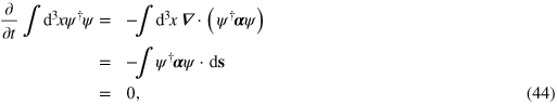

where  is identified as the probability current

This leads us to identify α as the velocity operator for the electron. The eigenvalues of the three operators, αx
, αy
and αz
are all  , which each correspond to the velocity of light. We can resolve this apparent conflict with experience by noting that a wave-packet formed by superposing energy eigenstates moves with the expected group velocity given by the ratio of the average momentum and the average energy. There is a remnant of the velocity eigenvalues in the rapid oscillations associated with the positive- and negative-energy components of the state. This, Zitterbewegung has a frequency in excess of
  or, equivalently, a spatial period comparable to the Compton wavelength of the electron.
2.1. Mechanical properties
The properties of an electron in relativistic quantum theory are represented by operators, just as in the more familiar non-relativistic theory. The position and momentum operators,  and
and  satisfy the canonical commutation relation

and the Dirac equation (12) leads directly to the Hamiltonian operator

This, together with the Heisenberg equation of motion, provides the evolution equations for the operators representing mechanical properties of interest. The position operator, for example, satisfies the equation

which we recognize as the velocity operator. The momentum operator commutes with the Hamiltonian and so, unlike the velocity operator, it is a constant of the motion

This demonstrates the conservation of momentum for a free electron.
It is with the angular momentum that the surprises begin, as the orbital angular momentum for a free electron is not conserved. We can define an orbital angular momentum operator precisely as in non-relativistic quantum theory

This operator does not commute with the Dirac Hamiltonian and so satisfies the non-trivial equation of motion

In contrast with the non-relativistic theory, the orbital angular momentum of a free electron, or of one confined a by a rotationally symmetric potential, is not a constant of the motion. Diracʼs resolution of this paradoxical situation was to add to the orbital angular momentum a spin angular momentum

Like the orbital angular momentum, this is not a constant of the motion, but satisfies the equation of motion

In relativistic quantum theory the spin and orbital angular momenta are naturally coupled together and it is only the total angular momentum, given by the sum of these, that is conserved. The total angular momentum operator

is a constant of the motion. It is this quantity, rather than the orbital or spin angular momenta, that appears in the relativistic expressions for atomic spectra [50, 51, 54]. We should note that the separation implicit in (25) is not, itself, Lorentz covariant.
2.2. Foldy–Wouthuysen transformation
It is apparent that the velocity operator for a Dirac electron is very different from that in non-relativistic quantum theory. This feature, together with the non-conservation of spin and orbital angular momentum and a desire to understand the non-relativistic limit motivated the discovery of a unitary transformation that diagonalizes the Dirac Hamiltonian [55]. The required unitary operator is generated by an Hermitian and time-independent operator, S, and has the form [51, 55]

where  is the magnitude of the momentum and θ is a parameter to be determined. It is not difficult to find that the required value of θ is

The Foldy–Wouthuysen transformation produces a new state and Dirac equation of the form
where  is the transformed (diagonal) Hamiltonian

The operator β has eigenvalues  , with the positive eigenvalue corresponding to the upper two components of ψ and the negative to the lower two. Clearly, the transformation has succeeded in separating the positive energy states from those with negative energy. The eigenvalues of
  , moreover, are
  in agreement with the relationship between energy, mass and momentum,
  , familiar from relativistic kinematics.
Our transformed Dirac equation has the form

If we consider only low energies in the non-relativistic regime then this, on making a binomial expansion, reduces to

If we further restrict our attention only to the two-component positive energy part of the state and shift our zero of energy, so as to remove the constant m term, then we recover the familiar Schrödinger equation for a free particle.
The operators representing the mechanical and other properties of the electron are also transformed by the Foldy–Wouthuysen transformation. In particular, the position operator  is transformed to [55]
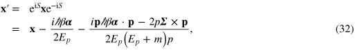
where Ep
is the operator  . The momentum operator commutes with S and so is unchanged by the transformation. The orbital and spin angular momenta are also changed by the Foldy–Wouthuysen transformation, with the orbital angular momentum operator becoming

The total angular momentum commutes with S and so is unchanged by the transformation. We can readily use this fact to obtain the transformed spin angular momentum operator. It is important to realize that using the transformed Hamiltonian, states and observables is entirely equivalent to working with the untransformed quantities and the original Dirac equation.
2.3. Mean properties
In the non-relativistic limit the position and momentum operators are  and
and  , as they are in the Dirac theory. With this non-relativistic limit in mind, it is reasonable to ask what role these operators play in the transformed system. We note that in the transformed picture, the original position operator satisfies the equation of motion

For a positive energy state this gives the velocity operator we might have expected:  . For a negative energy state the velocity is the same apart from an overall minus sign. The, Zitterbewegung or rapid oscillations, associated with an instantaneous velocity equal to that of light, has disappeared. For this reason, Foldy and Wouthuysen refer to the operator
  in their transformed system as the, mean-position operator. Working with this mean-position operator,
  , and the transformed Dirac equation (30) gives the familiar Schrödinger evolution in the non-relativistic limit. The other original operators
  and
Σ
are similarly the, mean-orbital and mean-spin angular momenta. It is important to note that it is these mean quantities that correspond to the those familiar from non-relativistic quantum theory [55].
and
Σ
are similarly the, mean-orbital and mean-spin angular momenta. It is important to note that it is these mean quantities that correspond to the those familiar from non-relativistic quantum theory [55].
The mean quantities can also be used with the original Dirac equation by simply inverting the Foldy–Wouthuysen transformation. This means, in particlar, that the mean position, orbital and spin angular momentum operators appropriate for use with the Dirac equation are, respectively,
echoing the quantities introduced by Pryce [56, 57]. The mean orbital and spin angular momenta, unlike their unaveraged counterparts, commute with the Hamiltonian and so are true constants of the motion. In the Foldy–Wouthuysen picture this means that

or, for the original Dirac Hamiltonian

3. Properties of the optical Dirac equation
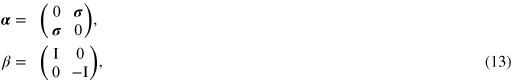
It is natural to ask if the Dirac equation can be applied to particles with spins other than the  associated with the electron [58] and an early application was to the (bosonic) mesons [59]. Our interest, of course, is the representation of the electromagnetic waves in Dirac form and to this end we rewrite our optical Dirac equation (9) in the form

where we associate the 'momentum' operator  with
with  and α is a vector the components of which are the 6 × 6 matrices

To these three matrices we add the 6 × 6 form of Diracʼs β-matrix

We have deliberately written these matrices using the same notation as that for the electron Dirac equation, so as to emphasize the similarities between them. The differences are apparent in the fact that the matrices for the optical Dirac equation are 6 × 6, rather than the 4 × 4 for the electron, and also that the commutation relations among the matrices are rather different [47, 59–65]. These are summarized in appendix
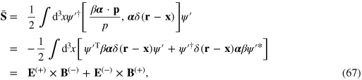
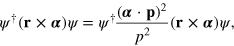
The optical Dirac equation leads to the same conservation law as for its electronic counterpart (15) but the relevant quantites are now the energy density 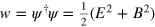 and the Poynting vector
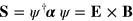
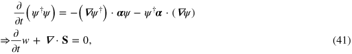
which we recognise as Poyntingʼs theorem. The difference in the dimensions of ψ for the electron and optical Dirac equations is manifested, here, in the change of meaning of the continuity equation from the local conservation of probability to the local conservation of energy.
3.1. Mechanical properties of light
The derivation of Poyntingʼs theorem as the continuity equation for the optical Dirac equation led us to identify the density of energy and the flux of energy, or the momentum density, as

To these we can add the density of the optical angular momentum, which we write as

We trust that no confusion will arise if we stick with established convention in which both the optical angular-momentum density and the electron probability current are represented by  . Each of these mechanical quantities is globally conserved, of course, and we should confirm this fact using the properties of our optical Dirac equation. The global conservation of energy follows directly from the local conservation law (41)
where we have used Gaussʼs theorem and the physical requirement that the fields tend to zero at infinity.
For the remaining properties we can proceed in the same way, using the Dirac equation for ψ and for  . Alternatively, we can exploit further the analogy between the (classical) optical Dirac equation and the (quantum) Dirac equation for the electron, by introducing the 'Hamiltonian' operator

and use Heisenbergʼs equation of motion. Let us emphasize that this is an entirely equivalent procedure to working with the optical Dirac equation itself and that, despite the appearance of ℏ, the description is essentially classical. The optical momentum, for example is, expressed in terms of the operator α and the momentum, density at position  therefore corresponds to the operator
  , where
  is the position operator, as before [66–68]. Both approaches lead to the same result. For the electromagnetic momentum density we find
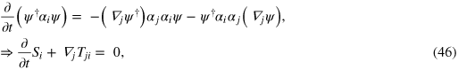
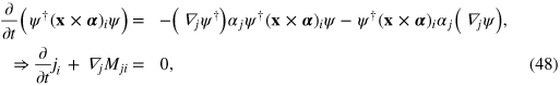
where we have introduced the summation convention in which a repeated index implies a summation over the three cartesian coordinates and Tji is the familiar momentum flux density [36]

In deriving the momentum continuity equation (46) we use the commutation properties of the Kemmer matrices, given in appendix  and
and  which mean that
 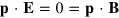 . If we follow the same procedure for the operator
  then we find the familiar local conservation for the electromagnetic angular momentum
where  is given by (43) and Mji
is the angular-momentum flux density [36, 69]
is given by (43) and Mji
is the angular-momentum flux density [36, 69]

3.2. Optical Foldy–Wouthuysen transformation
The expressions obtained in the preceding subsection are exact (within the Maxwell theory of the free field) and contain both rapidly and slowly oscillating contributions. For a monochromatic field of angular frequency ω, for example, the densities and flux densities of the energy, momentum and angular momentum include constant terms and terms oscillating at frequency  . In the majority of situations in optics, this frequency is too high to be observed in the interaction with matter and it is appropriate to remove the rapidly oscillating contributions so as to arrive at slowly-varying or mean properties. This process is known by different terms in different parts of optics: we may think of it as averaging over many optical cycles, the slowly-varying amplitude approximation or, within quantum optics, as making the rotating-wave approximation in the interaction with a detector. The situation is reminiscent and indeed precisely analogous to the, Zitterbewegung apparent in the physical quantities calculated from the Dirac equation for the electron. It is natural to construct the appropriate cycle-averaged optical properties by adopting the same procedure as for the electron: we apply a Foldy–Wouthuysen transformation to diagonalize the Hamiltonian for our optical Dirac equation and then seek suitable operators from which to obtain mean mechanical properties.
The optical Foldy–Wouthuysen transformation we seek is the natural analogue of that for the electron [47] with the required unitary operator having the form

where θ is a function, to be determined, of the, operator  . We can expand the unitary operator (50) in a form analogous to that given for the electron transformation in (26), although the form is complicated, somewhat, by the algebra of the Kemmer, as opposed to Dirac matrices. We find the form

where we define the operator

the properties of which are given in appendix
The desired diagonalized Hamiltonian is obtained by setting  , as shown in appendix
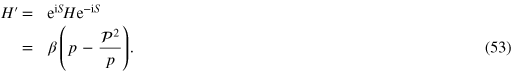
It follows that the eigenvalues of the Hamiltonian are  , corresponding to the wavenumber or angular frequency
  , as
, as  .
.
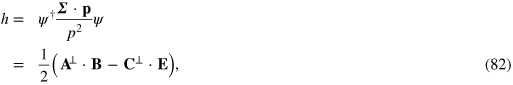
To complete the transformation we need to find the transformed spinor
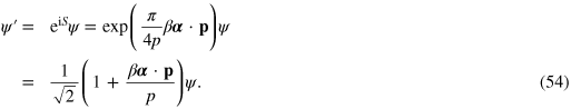
We can write this in terms of our electric and magnetic fields if we introduce complex electric and magnetic fields corresponding to the positive,  , and negative,
  , frequency parts of the field

where

These positive and negative frequency parts of the field are those that arise naturally in the theory of optical coherence and are associated, in the quantum theory of light, with the photon annihilation and creation operators respectively [70–72]. The transformed spinor naturally separates these components with positive frequency electric components in the top three entries and negative frequency components in the lower three

It is useful to note that the action of  on our transformed spinor gives the minus complex conjugate

and similary

We emphasize that the combination of this transformed spinor and the transformed Hamiltonian,  , is exact and fully equivalent to our untransformed quantities.
We conclude this subsection by noting that the paraxial approximation, a mainstay of laser physics [73, 74], is readily derived from our transformed optical Dirac equation. It follows from (53) and the transverse nature of the fields that our transformed Dirac equation has the form

There is no mass term, as in the corresponding equation for the electron (30), but we can arrive at a similar Schrödinger-like equation if one component of the momentum, which we take to be the z-component, is far larger than the others, so that  . In this case we write

If we make the ansatz

and multiply the equation by β, then our transformed Dirac equation becomes

so that cartesian components of the positive and negative frequency parts of both the electric and magnetic fields obey, in this approximation, a suitable paraxial wave equation [73, 74].
3.3. Mean optical properties
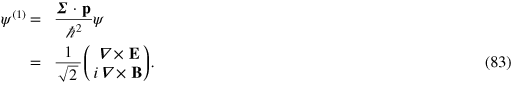
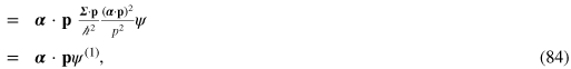
We can use our transformed spinor,  , to arrive at mean mechanical properties by following the procedure Foldy and Wouthuysen applied to the electron Dirac equation [55]. We transform the operators corresponding to the mechanical properties of interest and drop terms that are of odd order in the α, as these introduce cross terms between the positive and negative frequency parts of the spinor. This serves to remove the rapidly oscillating contributions in the same way as the corresponding procedure for the electron removes the, Zitterbewegung.
Let us begin by considering the energy density. We have transformed the spinor and our form for the energy density must be unchanged if we also transform the operator the expectation value of which is the energy density. It is straightforward to see that the operator for the energy density at position  must be
  , where
  is the position operator, as

Naturally, we obtain exactly the same result if we work with our transformed spinor  and the transformed energy density operator
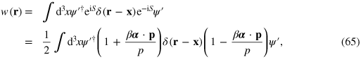
where we have used the fact that both  and
and  contain only transverse fields so that
  and
and  . We obtain the mean or cycle-averaged energy density by keeping only those terms that are of even order in α
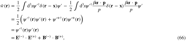
which is the required average. In reaching this result we have used the anti-commutation relation (A.1) and the complex-conjugation properties (58) and (59). This simple expression for the cycle-averaged energy density illustrates the benefit of working with the transformed spinor.
We can continue in the same way, by keeping terms of only even order in α to find the averaged forms of our other mechanical properties. For the momentum density we find
which is the required cycle-averaged form of Poyntingʼs vector. In reaching this expression, we have made use of the readily proved identity

The averaged momentum density (66), although evidently correct, is not in its most useful form. We can obtain a form closer to that used in optics [75] by evaluating the operator product  using (A.9). After a little work we find
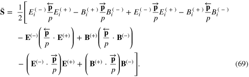
We recall that  and
and  and so write this in the simpler form
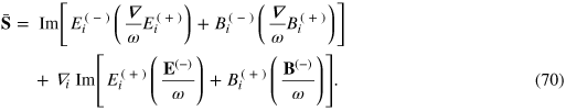
We emphasize that here ω is an, operator and that no restriction to monochromatic or near-monochromatic fields is necessary. The action of the operator  simply divides each temporal Fourier component of the field by its associated angular frequency. The second line in (70) is a divergence and therefore does not contribute to the total momentum density. It should be noted that this operator introduces some spatial averring in that, for example,
  is not simply related to
  at position
  alone. The density of a mechanical property is only defined up to such a divergence and so we are at liberty to neglect this term. If this statement needs justification, we recall that conserved quantities, like momentum, may be obtained from symmetries by means of Noetherʼs theorem and that the local resulting local conservation law only, defines the density up to a divergence [76–79]2
. We note, however, that retaining such divergence terms allows us to express the momentum density in a variety of suggestive forms [80], although, because of the non-uniqueness described above, it is difficult to assign to these any particular physical significance. If we drop the divergence term then we are left with the simple form
alone. The density of a mechanical property is only defined up to such a divergence and so we are at liberty to neglect this term. If this statement needs justification, we recall that conserved quantities, like momentum, may be obtained from symmetries by means of Noetherʼs theorem and that the local resulting local conservation law only, defines the density up to a divergence [76–79]2
. We note, however, that retaining such divergence terms allows us to express the momentum density in a variety of suggestive forms [80], although, because of the non-uniqueness described above, it is difficult to assign to these any particular physical significance. If we drop the divergence term then we are left with the simple form
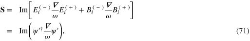
which is reminiscent of the momentum density in non-relativistic quantum theory [81], although the presence of the frequency operator, ω is an important difference.
4. Optical angular momentum
Our task, in this section, is to determine how the optical angular momentum, the orbital and spin components and the helicity arise from our optical Dirac equation. There are three reasons for undertaking this task. Firstly, of course, our discussion of the mechanical effects of light would not be complete without including angular momentum. Secondly angular momentum played an important role in the development of Diracʼs theory of the electron, in particular in determining the necessity of the existence of electron spin and its intimate relationship to the more familiar orbital angular momentum [48]. Finally optical angular momentum is currently a vibrant and active field of research [82–85] and we may hope that an enhanced understanding of optical angular momentum might be helpful in the further development of the field.
4.1. Spin and orbital components of the angular momentum
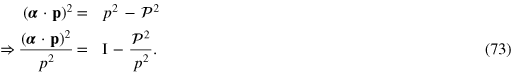
The problem of separating optical angular momentum into spin and orbital parts has an interesting history. It has been suggested, on theoretical grounds, that such a separation is not physically meaningful [86–91], and such a conclusion is, at first sight, natural as these quantities are not separately conserved for the Dirac electron [48]. This position is somewhat at odds, however, with experimental work which suggested, at least in some circumstances, that precisely such a separation is meaningful [92, 93]. The resolution of this apparent contradiction is that the separation of the total angular momentum into spin and orbital parts is indeed a physical one, but that neither the spin nor the orbital components is, by itself, an angular momentum [94, 95]. Both the spin and orbital parts are the generators of rotations that are constrained by the requirement that the rotated fields must be transverse [38, 39].
We have seen that the total angular momentum density is expressed, in the formalism of the optical Dirac equation in terms of the alpha matrices in the form

The spin and orbital parts of this total angular momentum are usually extracted by writing  in terms of the vector potential [94, 95] or both
  in terms of the vector potential and
  in terms of a second vector potential [38, 39] and using integration by parts. Here we make this division directly form the properties of the optical Dirac equation.
At first sight it is far from obvious how to break up  into constant spin and orbital parts. We achieve this by making use of a property of the Kemmer matrices (A.11)
We recall that  , by virtue of the transverse nature of the
  and
and  fields, and hence for any physically allowed fields we have

It follows that we are free to rewrite the total angular momentum density in the form
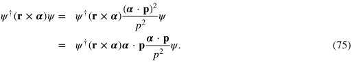
We proceed by evaluating the effect on ψ of the operator  In order to do so we introduce the transverse (divergenceless) and, gauge-invariant parts of two vector potentials,
  and
and  , related to our (transverse) electric and magnetic fields by [9, 96]
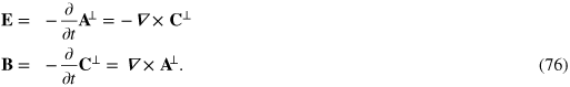
Hence with the aid of elementary vector identities we find

We can complete our calculation of the total angular momentum density by acting with  to the, left on
  . The result is

It is natural to identify these with the orbital, l, and spin, s parts of the angular momentum density and if we write these in terms of the fields and the potentials we find
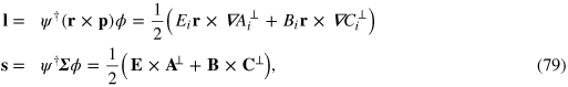
which we recognize as the required Heaviside–Larmor symmetric forms [38, 39, 78]. Had we chosen to act with  to the right we would have recovered
  and it follows that this expression and
  , given in (79), are, identical within the formalism of the optical Dirac equation. We note that, as for the electron, this separation into spin and orbital parts is not Lorentz-covariant.
We do not wish to give the impression that the spin and orbital angular momentum densities given in (79) are unique. Had we written
for example, then we would have obtained expressions for the densities differing only by a surface term, with the total volume-integrated spin and orbital angular momenta unchanged. The possibility of defining different densities for locally conserved quantities associated with the same total properties is familiar, of course, from Noetherʼs theorem [76–78].
4.2. Helicity
In particle physics, the helicity of a single particle is defined as the component of its spin along its momentum [52, 97–100], thus it is natural to define this as the expectation value of  . If we apply this idea to our optical Dirac equation then we are led to a helicity density in the form

It is certainly, possible to define the helicity in this way and, indeed, doing so has some practical advantages [101]. There are two clear reasons, however, why this does not suit our present purposes. The first is that it gives a value that is proportional to ℏ which should not appear in any physical quantity in our essentially classical analysis. The second, more serious, problem is that this quantity does not have the dimensions of an angular momentum density. We can remove both these features if we take our inspiration from (78) to give

but this quantity is a purely imaginary one.
We can recover the required form of the helicity density within from optical Dirac equation by defining the helicity operator to be  , so that the helicity density is
which is the familiar expression [40–45, 78]. The total helicity obtained by integrating this helicity density over all space is the conserved quantity associated with the Heaviside–Larmor symmetry and, in the quantum theory, is ℏ multiplied by the difference between the number of left and right circularly polarized photons.
The difference in form for the helicity operator in the optical Dirac when compared with the analogous quantity for the electron should not come as a surprise, as this has been true for each of the mechanical properties we have considered and has its origins in the fact that  has the dimensions of a probability density for the electron but an energy density for the electromagnetic field [16].
5. Zilch and higher-order conserved quantities
As a final application of the optical Dirac equation, we show how a class of further locally-conserved quantities, and in particular the Zilch [102, 103], arise naturally from it. These quantities have recently come to prominence in the study of chiral interactions [104–110].
We start by noting that if ψ is a solution of the optical Dirac equation, then so too is
The proof of this is straightforward, but instructive
where we have made use of (A.5). It follows that we can derive locally conserved quantities using  in place of ψ or, indeed, in combination with it. We present just one example

where Z000 is one of the components of Lipkinʼs Zilch [102].
We can extend the family of analogous conserved quantities indefinitely [40, 44, 78] by noting that the spinors

are also solutions of the optical Dirac equation. The repeated action of  generates successive curl operations on the fields and thereby produces locally conserved quantities that depend on derivatives of the fields of ever higher order.
It is also possible to extend the set of conserved quantities in the other direction, with successive 'inverse-curl' operations to produce the infra-zilches [44, 78]. These arise naturally on the introduction of a further class of spinors

These are clearly solutions of the optical Dirac equation and denoted with the superscript  by virtue of the fact that

so that the operators  acts on the
  as the, inverse of
  . The simplest new spinor,
  , has the form

The associated locally-conserved quantity  is simply the helicity density (82).
6. Conclusion
The formal connection between Maxwellʼs equations and the Dirac equation was noticed very soon after the latter was first derived and there is an extensive literature on the topic, much of it aimed at formulating a wavefunction for the photon [16, 21]. Our aim in this study has not been to address the quantum properties of light but rather to see what can be learnt about the classical electromagnetic field from the Dirac theory of the electron.
We have seen that many of the properties of light emerge naturally from the optical Dirac equation, including its principal mechanical properties and the associated conservation laws. The familiar operation of cycle averaging optical fields, moreover, is precisely analogous to the suppression of electron, Zitterbewegung and that the introduction of complex fields arises naturally from the Foldy–Wouthuysen diagonalization of the optical Dirac 'Hamiltonian'  . The separation of the angular momentum into spin and orbital parts appears naturally in this formalism as do the infinite sets of conserved quantities: the zilches and infra-zilches.
Analogies between optics and quantum theory are well established, of course. Indeed Gabor once wrote that 'optics was always considered as a good didactical preparation for wave mechanics, now it appears that quantum mechanics is not a bad preparation for optics' [111]. Perhaps, relativistic quantum theory is an even better one.
Acknowledgements
I thank Les Allen, Rob Cameron, Sarah Croke, Fiona Speirits and Alison Yao for their constructive comments and encouragement. This work was supported by the Engineering and Physical Sciences Research Council (EPSRC) under grant number EP/I012451/1, by the Royal Society and by the Wolfson Foundation.
Appendix A.: Properties of the Kemmer matrices
Useful properties of products of our spin-1 Kemmer (39) and (40) matrices follow from their commutators and anticommutators, the simplest of which is

The commutation relation for the alpha matrices is
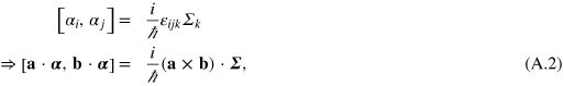
where εijk is the familiar alternating symbol and we have employed the summation convention in which indices appearing twice are summed over the three cartesian directions. The matix Σk is the k-component of the spin operator

Note the similarity with the electron operator (23). An important difference, of course, is that the electron operator has eigenvalues  but that our optical spin operator has eigenvalues
  . These spin matrices commute with β

The operators α and Σ are simply related by

The anticommutator of two alpha matrices is of a more complicated form that the commutator, and follows from the anticommutator of the tau matrices

where  is a symmetric three by three matrix with elements

We can combine this with the commutation relation (A.2) to write the product of two τ matrices in the form

so that

It is also useful to note a simple expression for products of three matrices [59]

We conclude with a list of properties of the matrices in combination with the momentum
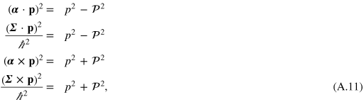
where  is the six by six matrix with dimensions p2

and Π is the three by three symmetric matrix with elements

Our ψ contains only transverse fields and this means that  acting on ψ give zero

Appendix B.: Optical Foldy–Wouthuysen transformation of the Hamiltonian
We seek a unitary transformation that diagonalizes the Hamiltonian operator for our optical Dirac equation. The transformed Hamiltonian has the form
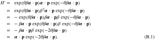
We can use the expanded form of the unitary operator (51) to write this as

To get a diagonal form we need to remove the  part and to this end we choose

The desired Hamiltonian is then

Footnotes
- 1
We use the term 'spinor' here to emphasize the analogy with Dirac spinors for the electron. Of course the strict meaning of the term is intimately associated with transformations, most especially the rotation and Lorentz groups, [29–31]. We do not claim to associate such properties with our ψ and do not associate it with a true spinor in this sense, but retain the term so as to emphasize the analogy with the electron.
- 2
It is beholden on me to alert the reader to two significant errors in the paper by Bliokh et al [79]. Firstly it is stated in their equation (3.36) that the, total spin and orbital angular momenta obtained from the conventional and dual-symmeric Lagrangians are different. They are not, as shown explicitly in [38]. Secondly, in their, note added, the authors, referring to the conventional and dual-symmetric Lagrangians, state that the choice makes a difference and has important physical consequences. It does not; both lead to the same Maxwell equations and are, therefore, physically indistinguishable. They have the same symmetries and conserved quantities as demonstrated in the appendix of [78].