


Abstract
The effects of physical interactions are usually incorporated into the quantum theory by including the corresponding terms in the Hamiltonian. Here we consider the effects of including the gravitational potential energy of massive particles in the Hamiltonian of quantum electrodynamics. This results in a predicted correction to the speed of light that is proportional to the fine structure constant. The correction to the speed of light obtained in this way depends on the gravitational potential and not the gravitational field, which is not gauge invariant and presumably nonphysical. Nevertheless, the predicted results are in reasonable agreement with experimental observations from Supernova 1987a.
Export citation and abstract BibTeX RIS

Content from this work may be used under the terms of the Creative Commons Attribution 3.0 licence. Any further distribution of this work must maintain attribution to the author(s) and the title of the work, journal citation and DOI.
1. Introduction
One might suppose that the effects of a gravitational field on a quantum system could be described, at least to a first approximation, by including the gravitational potential  in the Hamiltonian. That approach has been successfully used, for example, to analyze the results of neutron [1] and atom [2–10] interferometer experiments in a gravitational field. Here we consider a model in which
  is included in the Hamiltonian of quantum electrodynamics. As a result, virtual electron-positron pairs [11–16] have a gravitational potential energy that is the same as that of real particles. A straightforward calculation based on that assumption shows that the velocity of light in a gravitational potential would be reduced by an amount that is proportional to the fine structure constant
  .
.
The predicted correction to the speed of light depends on the gravitational potential and not the gravitational field, and it could be observed locally by comparing the velocity of photons and neutrinos, for example. As a result, the predicted correction to the speed of light is not gauge invariant. These results are also not equivalent to what would be obtained [17–19] from the currently-accepted generalization of the Dirac equation and quantum electrodynamics to curved spacetime [20–25]. The lack of gauge invariance and the disagreement with the generally-covariant Dirac equation both suggest that including the gravitational potential in the Hamiltonian must be nonphysical.
Nevertheless, the predicted correction to the speed of light from this simple model is in reasonable agreement with experimental observations from Supernova 1987a, where the first neutrinos arrived approximately 7.7 h before the first photons [26]. There is no conventional explanation for how that could have occurred and the currently-accepted interpretation of the data is that the first burst of neutrinos must have been unrelated to the supernova [26], despite the fact that the probability of such an event having occurred at random is less than  [27]. The predicted correction to the speed of light, if correct, could explain this long-standing anomaly.
Quantum mechanics and general relativity are two of the most fundamental laws of physics. Quantum mechanics has been verified to very high precision by quantum electrodynamics experiments such as the measurement of the electron g-factor [28, 29]. Experimental tests of general relativity are much more limited and many of the observed phenomena are consistent with other formalisms. As a result, there is currently a great deal of interest in performing high-precision tests [30] of general relativity using the properties of quantum systems, such as atom interferometers [2–10] superconductors [31–34], and photons [35, 36]. The correction to the speed of light predicted here is closely related to the equivalence principle, as will be described below, and these results may provide additional motivation for experimental tests of general relativity, especially the equivalence principle.
Einstein was the first to predict that the velocity of light would be reduced by a gravitational potential [37]. According to general relativity [38, 39], the speed of light  as measured in a global reference frame is given by

where  is the speed of light as measured in a local freely-falling reference frame. This reduction in the speed of light can be observed if a beam of light passes near a massive object such as the Sun, as illustrated in figure 1. The transit time from a distant planet or satellite to Earth can be measured as a function of the distance
  of closest approach to the Sun and then compared to the transit time expected at a velocity of
  . The results from such experiments [40] are in excellent agreement with the prediction of equation (1). The deflection of starlight by a massive object can also be intuitively understood in this way. It should be noted that the velocity of light measured by a local observer will be independent of
  and that the observable effects in this example are due to the spatial variations in
  .
.

Figure 1. A measurement of the transit time at the speed of light from a distant satellite to Earth. Einstein predicted that the speed of light as measured in a global reference frame would be reduced by the gravitational potential of the Sun as described by equation (1), which is in good agreement with experiments. Here  is the distance of closest approach. The deflection of the light beam by the gravitational potential of the Sun is very small and is not illustrated here.
Download figure:
Standard image High-resolution imageThe model considered here gives a correction to equation (1) that is proportional to the fine structure constant. These results are based on the Feynman diagrams [11–16, 41] of figure 2 as will be described in more detail below. Roughly speaking, the gravitational potential changes the energy of a virtual electron-positron pair, which in turn produces a small change  in the energy of a photon with wave vector
  as can be shown using perturbation theory. This results in a small correction to the angular frequency
  of a photon and thus its velocity
  . The analogous effects for neutrinos involve the weak interaction and they are negligibly small in comparison. As a result, this model predicts a small but observable reduction in the velocity of photons relative to that of neutrinos. In principle, the reduction in the speed of light could be directly measured by a local observer, but a small change in
  can be more easily observed by comparing the photon and neutrino velocities.

Figure 2. (a) A Feynman diagram in which a photon with wave vector  is annihilated to produce a virtual state containing an electron with momentum
  and a positron with momentum
  . After a short amount of time, the electron and positron are annihilated to produce a photon with the original wave vector
  . Any effect that this process may have on the velocity of light is removed using renormalization techniques to give the observed value of
  . (b) The same process, except that now the energies of the virtual electron and positron include their gravitational potential energy
  , as indicated by the arrows. This produces a small change in the velocity of light that is experimentally observable. The variable
  represents the time while
  represents the position in three dimensions (in arbitrary units).
Download figure:
Standard image High-resolution imageThe remainder of the paper begins with the motivation for including the gravitational energy  in the Hamiltonian of a quantum system. The correction to the speed of light due to the gravitational potential is then calculated using quantum electrodynamics and standard perturbation theory in section 3. Gauge invariance and the equivalence principle are discussed in section 4, while the predicted delay in the photon arrival time for Supernova 1987a is calculated in section 5 and compared with the experimental data. A summary and conclusions are presented in section 6. Appendix
2. Gravitational potentials in the quantum theory
In nonrelativistic quantum mechanics, the Hamiltonian  for a particle with mass
  in a Newtonian gravitational field is given by

where  is the Newtonian gravitational potential at position
  . Equation (2) has been successfully used to analyze the results of neutron interferometer experiments in a gravitational field, for example [1].
Equation (2) can be generalized to include the nonNewtonian gravitational effects of a rotating mass  by making use of the well-known analogy [33, 42–49] between electromagnetism and Einstein's field equations for a weak gravitational field. As outlined in appendix
  and a gravitational scalar potential
  that are determined by the metric. The motion of a classical particle is then described by the usual Lorentz force equation, which provides a convenient way to visualize general relativistic effects such as frame-dragging. This suggests that equation (2) can be generalized to

Equation (3) has previously been used in connection with the gravitational analog of the Aharonov–Bohm effect, for example [33, 47, 50–52]. We will be interested here in situations where the source of the gravitational field is stationary in the chosen coordinate frame, in which case  and equation (3) reduces to equation (2).
Equations (2) and (3) suggest that it may be possible to represent the effects of a weak gravitational field in quantum electrodynamics, at least to a first approximation, by including  in the usual interaction Hamiltonian
  . This gives
in the Lorentz gauge [12, 16]. Here the electromagnetic charge density  and current density
  are given as usual by
The charge of an electron is denoted by  ,
,  is the Dirac field operator,
  represents the Dirac matrices [53], and
  corresponds to the mass density of the particles as described in more detail in appendix
  and
and  represent the vector and scalar potentials of the electromagnetic field and the first two terms in equation (4) correspond to the usual interaction between charged particles and the electromagnetic field. The third term represents the gravitational potential energy of any particles. It is shown in appendix
  for both electrons and positrons. This is equivalent to the Schrödinger equation of equation (2) in the absence of a magnetic field.
For our purposes, the gravitational potentials  and
and  will be assumed to be classical fields. Similar results would be obtained if a weak gravitational field were quantized to introduce gravitons, as is illustrated in figure 3.
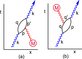
Figure 3. Feynman diagrams that are equivalent to those of figure 2 except that here gravity is quantized and the gravitational potential is produced by the emission and absorption of virtual gravitons. (a) A graviton produced by mass  is absorbed by a virtual electron, changing its momentum from
  to
to  . (b) A virtual positron emits a graviton that is then absorbed by mass
  . The momentum of the positron is changed from
  to
to  . Two other diagrams (not shown) involve the emission of a graviton by a virtual electron or the absorption of a graviton by a virtual positron.
Download figure:
Standard image High-resolution imageEquation (4) represents a simple model in which the gravitational potential of any massive particles is included in the Hamiltonian. Although this assumption seems plausible, it leads to an observable correction to the speed of light that is not equivalent to what is obtained using the currently-accepted generalization of the Dirac equation to curved spacetime [17–19]. The fact that the predictions of this simple model are in reasonable agreement with experimental observation may provide some motivation for considering the differences between these two approaches.
3. Calculated correction to the speed of light
In quantum electrodynamics, there is a probability amplitude for a photon propagating in free space with wave vector  and angular frequency
  to be annihilated while producing a virtual state containing an electron-positron pair, as illustrated in figure 2(a). The virtual state only exists for a brief amount of time, after which the process is reversed and the electron-positron pair is annihilated and the original photon is reemitted. This process, which is known as vacuum polarization [54], leads to divergent terms that can be eliminated using renormalization techniques while small corrections to this process can produce observable effects.
Here we will calculate the change  in the energy of a photon with wave vector
  due to the interaction of a virtual electron-positron pair with the gravitational potential as illustrated schematically in figure 2(b). The gravitational potential changes the energy of the virtual electron–positron state by
  , as is shown in appendix
  ) of a photon on
  will produce a correction to its velocity
  . It will be assumed here that the gravitational field is not quantized and is described by the Newtonian potential
  .
.
From second-order perturbation theory [53], the change  in the energy of a photon with wave vector
  is given by

Here  represents the unperturbed initial state containing only the photon while
  represents all possible intermediate states containing an electron-positron pair. The unperturbed energy of the initial state is represented by
  while
while  is the unperturbed energy of the intermediate state. For the purposes of this calculation, the gravitational potential term in equation (4) will be included in the unperturbed Hamiltonian
  while the electromagnetic interaction terms will be included in the perturbation Hamiltonian
  . As a result, the unperturbed energy of the intermediate state containing an electron-positron pair becomes
  . Here
  and
and  are the momenta of the virtual electron and positron respectively, as in figure 2, while
  is the relativistic energy of a free particle given as usual by
  .
.
Straightforward perturbation theory will be used for simplicity and because the usual Feynman diagram rules [11–16] may not be directly applicable to the Hamiltonian of equation (4). Equation (6) corresponds to steady state perturbation theory, but the same results can be obtained using the forward-scattering amplitude from time-dependent perturbation theory [53].
We will use periodic boundary conditions with a unit volume  [55]. In the Schrödinger picture, the Dirac field operators are then given by [15]

Here  creates an electron with momentum
  and spin
  , whose values will be denoted by ± to indicate spin up or down, while
  creates a positron with momentum
  and spin
  . The Dirac spinors
  and
and  are defined [14, 15, 53] by
where  .
.
The scalar electromagnetic potential  and the longitudinal part of
  do not contribute to this process. In Gaussian units, the transverse part of the electromagnetic vector potential operator is given by

Here  and
and  denotes two transverse polarization unit vectors. Without loss of generality, we can assume that the initial photon has its wave vector
  in the
  direction with its polarization along the
  direction.
The integral over  in the interaction Hamiltonian of equation (4) combined with the exponential factors in
  ,
,  , and
, and  give a delta-function that conserves momentum, so that
  and the sum over intermediate states reduces to a sum over all values of
  . We will assume that the energy of the photon is sufficiently small that
  , in which case
  (i.e., the recoil momentum from absorbing the photon has a negligible effect on the virtual particle energies). For the same reason, we can approximate
  by
by  in the evaluation of
  with the result that
with similar results for the other spin states. Here we have made use of equation (8) and the fact that
in the usual representation. Equation (10) was derived by simply multiplying the relevant matrices and vectors, while the same results could have been obtained more generally by using the properties of the Dirac matrices. Combining these results with equations (4), (7), and (9) gives
for the spin combination of equation (10).
Inserting equation (12) into equation (6) and summing over all of the intermediate spin states gives the correction to the photon energy as

Here we have introduced the fine structure constant  and the factor of
  comes from converting the sum to an integral. The notation
  has been used here to indicate that it is the unperturbed photon energy
  that appears in equation (13).
We can now use the assumption that  and
and  to expand the denominator in the first term inside the integral of equation (13) in a Taylor series to first order in
  and to second order in
  . This gives
We have only retained terms proportional to  in equation (14), since we are only interested in the first-order effects of the gravitational field.
We will first consider the effects of the last term in equation (14) and then return to consider the remaining two terms. The contribution from the last term gives
Evaluating the integral gives

The velocity of light is given by  and the correction
  to
to  is thus

Inserting the value of  from equation (16) into equation (17) gives

Equation (18) is the main result of this paper. Since  is negative, this gives a small reduction in the speed of light.
Returning to the first and second terms on the right-hand side of equation (14), it can be shown that their contributions to  are proportional to
  and
and  , respectively. These are nonphysical terms that become infinite in the limit of long wavelengths, which is somewhat similar to the usual infrared divergences encountered in quantum electrodynamics. We can make an intuitive argument that these terms should vanish as a result of renormalization as follows: The loop diagram of figure 2(a) would give an infinite correction to the energy of a photon, so that the 'bare' energy
  of the photon must be infinitely large as well. Identifying
  with
with  would therefore cause the nonphysical terms that involve
  and
and  to vanish, whereas
  cancels out of the finite correction of equation (17). A more rigorous treatment of renormalization would clearly be desirable, but that may not be possible in view of the fact that quantum gravity appears to be nonrenormalizable.
A neutrino can also undergo a virtual process in which particles such as W bosons, Z bosons, and leptons are created, after which the virtual particles are annihilated to give back the original neutrino state. The energy of the particles in the intermediate state will include their gravitational potential energy  , which will produce a small correction to the velocity of a neutrino that is analogous to that of a photon calculated above. But this process involves the weak interaction where the matrix elements are many orders of magnitude smaller than those for the electromagnetic interaction responsible for virtual electron-positron pair production. As a result, the expected correction to the velocity of neutrinos is negligible compared to that of photons.
4. Gauge invariance and the equivalence principle
Before we consider the magnitude of this effect, it is important to note that the results of this calculation are not gauge invariant with respect to the gravitational field. Conventional quantum electrodynamics is gauge invariant only because charge is conserved via

As a result, creating an electron-positron pair in a region of uniform electrostatic potential has no effect on the total electrostatic energy of the system because there is no change in the total charge, as illustrated in figure 4(a). But the Hamiltonian of quantum electrodynamics does not conserve the mass of the system in a virtual state containing an electron-positron pair and there is no equivalent of equation (19) for mass in that case, as is discussed in more detail in appendix
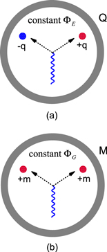
Figure 4. Effects of a constant electrostatic or gravitational potential on the energy of the electron-positron pair produced in the Feynman diagrams of figures 2 and 3. (a) A region of constant electrostatic potential  is created using a uniform spherical charge distribution with a total charge of
  . The energy of an electron-positron pair is unaffected by
  because the total change in the charge is zero as required by equation (19). (b) A region of constant gravitational potential
  is created using a uniform spherical mass distribution with a total mass of
  . Now the energy of the electron-positron pair is changed by
  because the pair production process does not conserve mass. There is no equivalent of equation (19) in this case.
Download figure:
Standard image High-resolution imageBased on the equivalence principle [38, 39, 56], one would expect that these effects should vanish in a local freely-falling reference frame. The calculations described above were performed using a coordinate frame that was assumed to be at rest with respect to mass  , where it seems reasonable to suppose that the effects of gravity can be represented by the Feynman diagrams of figures 2(b) or 3. In that reference frame, the photons and neutrinos would travel at different velocities according to equation (18). If we made a transformation to a local freely-falling coordinate frame where the laws of physics are assumed to be the same as in the absence of a gravitational field, then the photons and neutrinos would be expected to travel at the same velocity. This leads to a contradiction, since there can be no disagreement as to whether or not two particles are traveling at the same velocity. Thus the Hamiltonian of equation (4) leads to a small departure from the equivalence principle, which is closely related to the lack of gravitational gauge invariance noted above.
It has been predicted [57, 58] that electrons with spin up and spin down will fall at different rates in a gravitational field in apparent violation of the weak equivalence principle. (This effect is analogous to the spin–orbit coupling of an electron moving in the Coulomb field of an atom.) That may not be too surprising given that a classical object with nonzero angular momentum will exhibit similar effects [58, 59]. But the fact that an electron is a point particle makes this situation different from that of a gyroscope whose finite extent makes it susceptible to tidal forces, for example. The weak equivalence principle is sometimes stated as only applying to point particles with zero angular momentum, in which case it should not be applied to electrons. This raises some questions regarding the assumptions that are inherent in the derivation of the generally covariant form of the Dirac equation. In any event, the predicted correction to the speed of light from equation (18) provides further motivation for experimental tests of the equivalence principle.
5. Comparison with experimental observations
The first neutrinos from Supernova 1987a arrived 7.7 h before the first photons. The currently-accepted interpretation [26] of this data is that the first burst of neutrinos must not have been associated with the supernova because there is no conventional explanation for how the neutrinos could have arrived at that time. If equation (18) is valid, it could explain this long-standing anomaly.
The value of  is needed in order to compare the predicted correction to the speed of light with experimental observations such as those from Supernova 1987a. The Newtonian gravitational potential from an object with mass
  at a distance
  is given by

where  is the gravitational constant. Table 1 shows the approximate value of
  and the corresponding correction to the speed of light from equation (18) for the case in which the source of the gravitational potential is the Earth, the Sun, or the Milky Way galaxy. It can be seen that the contributions to the gravitational potential from the Earth and Sun are negligible compared to that of the Milky Way galaxy.
Table 1.
Gravitational potential  and fractional correction to the speed of light
  from the Earth, the Sun, and the Milky Way galaxy. The value of the gravitational potential from the Milky Way galaxy was approximated at the location of the Earth using equation (20).

|

|
|
|---|---|---|
| Earth |

|

|
| Sun |

|

|
| Galaxy |

|

|
The gravitational potential  from the Universe as a whole is not given by the Newtonian formula of equation (20). Instead,
  for a flat universe as is discussed in appendix
Supernova 1987a was located in the Large Magellanic Cloud [60], which is a smaller galaxy that is gravitationally bound to the Milky Way galaxy. In order to predict the expected difference in the arrival times of photons and neutrinos at the Earth, it is necessary to integrate the effects of equation (18) over their path which is illustrated in figure 5. Longo [61] integrated the usual relativistic factor of  in equation (1) over the path illustrated in figure 5 using a model for the gravitational potential produced by the Milky Way galaxy. (The contribution of the Large Magellanic Cloud to the gravitational potential is negligible due to its small mass.) He obtained a total time delay of 3506 h from the usual correction to the speed of light in equation (1). A similar calculation by Krauss and Tremaine [62] gave a total time delay of 3944 h.

Figure 5. Path followed by the neutrinos and photons from Supernova 1987a, which was located in the Large Magellanic Cloud [62]. [61] and [62] estimated the time delay expected from equation (1) using the gravitational potential from the Milky Way galaxy, which can then be used to calculate the contribution from equation (18).
Download figure:
Standard image High-resolution imageThe integral of equation (18) over the same path differs from these estimates by a factor of  and also by a factor of
  , since the factor of 2 in equation (1) does not appear in equation (18). Applying this factor to the average of the results of Longo [61] and of Krauss and Tremaine [62] gives a predicted delay of 1.9 h for the photons relative to the neutrinos based on equation (18). This estimate is really a lower bound on the actual delay, since refs. [61] and [62] only included the mass of the Milky Way that is within 60 kpc of the center of the galaxy. That represents roughly half of the estimated mass of the galaxy and the predicted delay could be as large as 4 h if the additional mass were included. (The effects of dark matter appear to be included in [61] and [62] and no correction for that is required.)
The observations made during Supernova 1987a are illustrated in figure 6, which is based on a review article by Bahcall and his colleagues [26]. A burst of neutrinos was observed by a detector underneath Mont Blanc followed 4.7 h later by a second burst of neutrinos that was detected in the Kamiokande II detector in Japan and the IMB detector in Ohio. The first observation of visible light from the supernova was then observed approximately three hours after the second burst of neutrinos, or 7.7 h after the first burst of neutrinos. As mentioned earlier, the usual interpretation of this data is that the first burst of neutrinos must not have been associated with the supernova for the reasons described below.

Figure 6. Sequence of events observed during Supernova 1987a [26]. The time at which the first burst of neutrinos was observed in the Mont Blanc detector is indicated by the dashed line, while the time at which the second burst of neutrinos was observed in the Kamiokande II and IMB detectors is indicated by the dotted-dashed line. The data points show the magnitude (logarithmic intensity) of the observed visible light from the supernova as a function of the time (in days) after the arrival of the second burst of neutrinos. The solid line is the result of a numerical calculation based on the accepted model of the supernova. The first burst of neutrinos was considered to be inconsistent with the accepted model and was rejected as a statistical outlier [26]. This discrepancy could be explained if the arrival of the photons was delayed as predicted by equation (18).
Download figure:
Standard image High-resolution image
A numerical simulation of the collapse of the progenitor star gave a predicted visible light intensity as a function of time (light curve) that is represented by the solid line in figure 6. There is an expected time delay of approximately three hours between the collapse of the core and the production of visible light at the surface of the star due to the propagation of a shock wave through the stellar material. (Any light produced in the interior of the star will be prevented from immediately reaching the surface due to diffusion). As a result, Bahcall and his colleagues have stated that the arrival time of the first burst of neutrinos 'is not consistent with the observed light curve' [26]. In addition, the fact that the first burst of neutrinos was only detected by the Mont Blanc detector and not the other two detectors, which were assumed at the time to have higher sensitivities, further suggested that the first burst of neutrinos must have been an anomaly that was not associated with Supernova 1987a [26].
The probability that the detection of the initial burst of neutrinos in the Mont Blanc detector was a random occurrence has been estimated to be less than  [27]. As a result, there are some experts in the field who consider the origin of the first burst of neutrinos to be an open question [27, 63–65]. A more recent numerical simulation [65] showed that a progenitor star with a sufficiently high rate of angular rotation would be expected to produce an initial incomplete collapse of the core followed by a second collapse, which would produce two bursts of neutrinos instead of just one. In addition, the simulation showed that different kinds of neutrinos with different energy ranges should have been produced during the two collapses [64, 65]. The material used in the Mont Blanc detector was different from that used in the other two detectors and the expected sensitivity of detection for the kind of neutrinos in the first burst has been estimated to be a factor of 20 higher in the Mont Blanc detector than the other detectors, which is consistent with the observations [64].
The possibility of a double collapse of the core suggests an alternative explanation for the observations associated with Supernova 1987a. In this scenario, the first burst of neutrinos signaled the initial collapse of the core with an associated production of visible light roughly 3 h later as expected from the models. If the photons were delayed by an additional 4.7 h by the gravitational potential in equation (18), then the light would have arrived 7.7 h after the first neutrino burst, as observed. The second collapse of the core would have produced an increase in the intensity of the visible light approximately 4.7 h after the arrival of the first photons. This is consistent with the observation that the light signal increased more rapidly than would have otherwise been expected during that time interval [26].
The photon delay of 1.9 h relative to the neutrinos as predicted by equation (18) is only 40% of the 4.7 h delay assumed in the scenario described above. As mentioned earlier, this estimate is a lower bound on the actual delay which could be as large as 4 h. Thus equation (18) is in reasonable agreement with the experimental observations and it provides a possible explanation for the first burst of neutrinos that is inconsistent with the conventional model of the supernova.
The Hamiltonian of equation (4) does not appear to be ruled out by the results of existing high-precision tests of quantum electrodynamics [66]. It would result in a small correction to the anomalous magnetic moment of the electron, for example, that is much smaller than the precision of the current experiments [28, 29]. The model would also predict [66] a correction to the decay rate of orthopositronium that is approximately two orders of magnitude smaller than the current experimental precision [67]. Future experiments of that kind may eventually allow an independent test of the implications of including the gravitational potential in the Hamiltonian.
6. Summary and conclusions
A simple model has been considered here in which it was assumed that, to a first approximation, the effects of a weak gravitational field on a quantum system can be represented by including the gravitational potential energy of any massive particles in the Hamiltonian. When applied to the Hamiltonian of quantum electrodynamics, this results in virtual electrons and positrons having a gravitational potential energy that is the same as that of a real particle. Perturbation theory was then used to show that such a model predicts a small reduction in the speed of light while the corresponding effects for neutrinos are negligibly small due to their weak interactions.
The predicted correction to the speed of light depends on the gravitational potential and not the gravitational field. An observable difference between the velocity of photons and neutrinos that depends only on the gravitational potential is not gauge invariant. The origin of this lack of gauge invariance can be understood from the fact that the gravitational potential energy has the same sign for the virtual electrons and positrons created during pair production, while their electrostatic potential energies have the opposite sign and cancel out, as illustrated in figure 4.
The predictions of this simple model are also in disagreement with the analogous calculations performed using the generalization of the Dirac equation to curved spacetime, which gives a much smaller effect that does depend on the gravitational field and not the potential itself [17–19]. The lack of gauge invariance and the disagreement with the generally-covariant form of the Dirac equation both suggest that this simple model must be nonphysical.
Nevertheless, the predictions of this model are in reasonable agreement with the experimental observations from Supernova 1987a, in which the first neutrinos arrived 7.7 h before the first photons. There is no conventional explanation for how that could have occurred and the currently-accepted interpretation is that the first burst of neutrinos must not have been related to the supernova [26], despite the fact that the probability of such an event occurring at random has been estimated to be less than  [27]. The correction to the speed of light from equation (18), if correct, would explain this anomaly.
The differences between this simple model and the generally covariant form of the Dirac equation are closely related to the role of the equivalence principle, since photons and neutrinos should travel at the same velocity in a local freely-falling reference frame and thus in all reference frames. (The rest mass of a high-energy neutrino is negligible in this regard.) There is already considerable interest in experimental tests of the equivalence principle and the results of the model considered here may provide further motivation for experiments of that kind.
Quantum mechanics and general relativity are two of the most fundamental laws of physics. Combining these two theories in a consistent way is currently one of the major goals of physics research. The predicted correction to the speed of light in a gravitational potential may be of further interest if the currently-accepted principles of quantum mechanics and general relativity are eventually found to be incompatible in some way.
Acknowledgements
I would like to acknowledge stimulating discussions with W Cohick, A Kogut and D Shortle.
Appendix A.: Gravitational potentials in general relativity
This appendix briefly reviews the analogy between general relativity and electromagnetism for a weak gravitational field, which leads to the introduction of the gravitational analogs of the electromagnetic vector and scalar potentials. The field equations of general relativity are nonlinear but they can be linearized if the gravitational field is sufficiently small [33, 38, 39, 42–49]. In that case, we can write the metric tensor  in the form

where  is the diagonal metric of special relativity with elements of
  and
and  is assumed to be small. It will also be convenient to define
  and
and  by
by
We can then define [43–45, 49] the gravitational vector and scalar potentials  and
and  by
by
We can also define two vectors  and
and  by
by

Einstein's field equations can then be used to show that

where  and
and  are the mass density and current. The potentials can be also be shown to obey the wave equations
Equations (A.4) through (A.6) are the same as those of classical electromagnetism except for the factor of  and the sign of the source terms.
The geodesic equation can also be used to show that the trajectory of a particle of mass  is given [43–45, 49] by

in the limit of low velocities. Here  is the gravitational force and equation (A.7) is the same as the Lorentz force in electromagnetism except for the factor of 4. Some authors redefine a new vector potential
  and a new gravitomagnetic field
  in order to put equation (A.7) into the same form as in electromagnetism. In that case the wave equation of (A.6) no longer holds in its present form. This factor of 4 is due to the fact that the gravitational field is a tensor and not a vector, and its appearance somewhere in the equations is unavoidable.
One of the most interesting and fundamental features of the quantum theory is the fact that it is the electromagnetic potentials  and
and  , not the electromagnetic fields
  and
and  , that appear in the Hamiltonian for a charged particle [53]. This gives rise to the Aharonov–Bohm effect [50] in which there are observable phenomena that occur in regions of space where
  and
and  , for example. This and the Lorentz force equation (A.7) both suggest that the Hamiltonian for a nonrelativistic particle in a weak gravitational field should be taken to be

in analogy with electromagnetism. Equation (3) in the text results from replacing the vector potential with  . Equation (A.8) has previously been used in connection with the gravitational analog of the Aharonov–Bohm effect [33, 47, 50–52], for example.
It can be seen from equation (A.3) that the gravitational potential  from the Universe as a whole is zero for a flat universe where
  aside from the effects of local mass density variations. This justifies the assumption in the main text that the total mass of the Universe does not contribute to the correction to the speed of light as might be expected from the Newtonian expression of equation (20).
Appendix B.: Mass density operator and the nonrelativistic limit
It was assumed in the text that the gravitational potential energy of a virtual electron-positron pair is  while the electrostatic potential energy cancels to zero. This difference between
  and
and  is responsible for the predicted correction to the speed of light as well as the lack of gauge invariance in figure 4. The purpose of this appendix is to define a mass density operator
  with these properties. The nonrelativistic limit of the interaction Hamiltonian of equation (4) is then shown to reduce to the Pauli equation with the correct sign of the gravitational potential energy for both electrons and positrons.
The electric charge and current densities can be written in covariant form as a four-vector  , whose fourth component is c times the charge density
  . Here the
  are the usual Dirac matrices and
  is the adjoint field operator, where
  is given as usual by
Roughly speaking, the minus signs in  ensure that a positron will have the opposite charge from an electron. Since we want the gravitational potential to have the same sign for both electrons and positrons, this suggests that the simplest choice for
  may be

This differs from  by the absence of
  which would be expected to give a positive gravitational potential for both electrons and positrons.
We will first investigate the nonrelativistic limit of the interaction Hamiltonian in equation (4). Combining  with the remaining noninteracting terms in the Hamiltonian and inserting
  from equation (B.2) gives the total Hamiltonian
  :
:
This is the standard Hamiltonian of quantum electrodynamics [68] aside from the  term. The time dependence of
  in the Heisenberg picture can be calculated using the anti-commutation property
  , which gives [68]

This is the usual Dirac equation for the second-quantized field operator with the addition of the gravitational potential term.
The nonrelativistic limit of equation (B.4) can now be calculated using the approach described in ref. [53], for example. We first rewrite the four-component field operator in the form
where  and
and  are two-component spinors. The Dirac equation (B.4) is then equivalent to
where  denotes the Pauli spin matrices. If we consider a positive-energy eigenstate corresponding to an electron with a velocity
  , then
  when acting on that state and the second line of equation (B.5) gives to lowest order

Here we have assumed that the potential energies are small compared to the rest mass and that the time rate of change of the state is  to lowest order [53]. Inserting equation (B.7) into the first line of equation (B.6) and using the identity

gives

This is the usual Pauli equation written in terms of (nonrelativistic) second-quantized field opertors [53] with the addition of the gravitational potential term.
If we consider an eigenstate corresponding to a positron instead, then  when acting on that state and the first line of equation (B.6) gives to lowest order

Inserting this into the second line of equation (B.6) gives

This can be rewritten by defining a new operator  (charge conjugation) and taking the adjoint of equation (B.11), which gives

Equation (B.12) corresponds to the Pauli equation for a particle (a positron) whose charge and spin are opposite that of an electron but whose mass and gravitational potential energy are the same as that of an electron. Taking  gives the nonrelativistic Schrödinger equation of equation (2) as desired. Equations (B.9) and (B.12) show that this choice of
  gives the correct sign of the gravitational potential energy for both electrons and positrons at least in the nonrelativistic limit.
We now generalize this to the case in which the virtual electron-positron pair may have relativistic velocities. Here we make use of the fact that, in the text, the gravitational potential was included in the unperturbed Hamiltonian  , where
  . The perturbation calculations were then based on the eigenstates of
  and their corresponding energy eigenvalues
  , which were assumed to include a gravitational potential energy of
  for each particle. First consider the value of the eigenvalue
  for a positron state
  with momentum
  and spin
  , where
  is the vacuum. For a weak field with
  , the gravitational contribution
  to the eigenvalue
  is given [53] to lowest order in perturbation theory in
  by
by

Here we have used the gravitational potential term in the Hamiltonian of equation (4) and inserted the definition of  from equation (B.2). Using the form of
  from equation (7) gives the relevant terms in
  as
as
Here the order of the operators  and
and  were interchanged using their anti-commutator. The term involving the Kronecker delta function is a constant (nonoperator) that is independent of the state of the system and can be ignored [68]. (This procedure is also necessary in order to obtain the correct charge of a positron.) Inserting equation (B.14) into equation (B.13) gives
The right-hand side of equation (B.15) follows from the fact that  [12, 14, 15].
It can be seen from equation (B.15) that a positron will have a gravitational potential energy with the correct sign but multiplied by a relativistic factor that depends on the value of  . This can be avoided if we define a new set of spinors
  and
and  that are defined by
We also define the operator  by
by

where the spinors of equation (B.16) have been inserted into equation (7). The definition of  in equation (B.2) is now replaced by

while the usual field operator  is used in
  and
and  .
.
With this choice of  , equation (B.15) becomes

and the energy of a positron in a gravitational potential is  as desired. The same result can also obtained for the energy of an electron. This justifies the assumption in the text that a virtual electron-positron pair has a gravitational potential energy of
  .
.
The nonrelativistic limit is not affected by this new definition of  because
  in that limit and equations (B.9) and (B.12) remain valid. It can also be shown that the expectation value in the state
  of the integral of
  over all space is equal to the mass
  as would be expected.
It should be emphasized that the model described in this paper is only intended to provide an alternative and approximate description of the propagation of photons in a gravitational potential; it is not intended to represent a complete or consistent theory. For example,  cannot obey a conservation law as a result of pair production and it is not part of a covariant four-vector. A more rigorous discussion of related issues in the currently-accepted formulation of the Dirac equation in curved spacetime will be submitted for publication elsewhere.