


Abstract
Long-living coupled transverse and longitudinal phonon modes are explored in dense, regular arrangements of flattened microfluidic droplets. The collective oscillations are driven by hydrodynamic interactions between the confined droplets and can be excited in a controlled way. Experimental results are quantitatively compared to simulation results obtained by multi-particle collision dynamics. The observed transverse modes are acoustic phonons and obey the predictions of a linearized far-field theory. The longitudinal modes arise from a nonlinear mode coupling due to the lateral variation of the confined flow field. The proposed mechanism for the nonlinear excitation is expected to be relevant for hydrodynamic motion in other crowded non-equilibrium systems under confinement.
Export citation and abstract BibTeX RIS

Content from this work may be used under the terms of the Creative Commons Attribution 3.0 licence. Any further distribution of this work must maintain attribution to the author(s) and the title of the work, journal citation and DOI.
1. Introduction
Hydrodynamic interactions of solute objects in driven non-equilibrium systems lead to complex phenomena such as strong correlations in sedimenting suspensions [1], shock-waves in two-dimensional disordered ensembles of droplets [2], or cluster formation and alignment of red blood cells in micro-capillaries [3]. The dynamics of non-equilibrium many-body systems can be favorably studied in microfluidic systems using ordered arrangements of flowing droplets (microfluidic crystals) [4, 5]. In pioneering studies, Beatus et al [6–8] observed collective vibrations in trains of disk like droplets flowing in a microfluidic Hele–Shaw configuration. These oscillations have been characterized as acoustic phonons with properties similar to lattice modes in dusty-plasma crystals [9]. Their dispersion relation has been obtained to linear-order in terms of a small-amplitude expansion of the ensemble flow [6, 7]. However, in contrast to solid-state phonons that can be excited in a controlled way by mechanical or optical means, microfluidic phonons have so far been observed only when excited by spontaneous asymmetries or defects in microchannels [6–8]. Possible nonlinear effects and interactions between phonon modes could not be studied systematically in these settings [8, 10].
In this work, we broaden the possibility to study hydrodynamically mediated collective phenomena by exploring dense droplet systems, where spherical droplets are only slightly flattened and nearly in contact to each other. We demonstrate that long-living transverse phonon modes can be systematically excited. The controlled excited transverse phonon modes oscillate between the confining channel walls which define the preferred oscillation mode. Moreover, the non-vanishing transverse amplitude gives rise to nonlinearly coupled longitudinal oscillations which are beyond the acoustic longitudinal modes observed in previous works [6–8]. The experimental measurements are confirmed by results from computer simulations using a mesoscale hydrodynamics approach which is able to reproduce the full nonlinear interactions. While a linearized far-field approximation describes the transverse phonon modes of the dense droplet trains surprisingly well, the observed longitudinal modes reveal a nonlinear coupling due to the influence of the confinement on the dense droplet crystal. This type of hydrodynamic coupling has impact on the self-organization in crowded non-equilibrium systems, and is thus relevant, e.g., for controlling particle flow in applications such as microfluidic cytometry [11]. In such systems, the mild vertical confinement we explore is more realistic than the extreme confinement of [7, 8].
2. Experimental setup and simulation method
Microfluidic devices to explore the collective droplet oscillations were fabricated in Sylgard 184 (Dow Corning) and bonded to glass microscopy slides using standard soft lithographic protocols [12, 13]. The flow rates were volume-controlled using computer controlled syringe pumps. Mono-disperse water droplets with radius  are generated in n-hexadecane (
 ,
,  ) with 2 wt% of the surfactant Span 80 using a step-emulsification geometry [13, 14], cf figure 1(a). The spacing of the droplets in the regular trains (crystal spacing) is
  , i.e.
  . The microchannel has uniform height and width of
  . The size of the droplets exceeds the height H of the microfluidic channel such that the droplets are flattened, and the drag coefficient in this case scales with
  [8]. Typical flow velocities are
  for the droplet, and
  for the continuous oil phase, as observed directly from microscopy images, respectively calculated from the applied volumetric flow rates. The corresponding Reynolds and Peclet number are
  and
and  , where
  is the diffusion coefficient of a droplet.
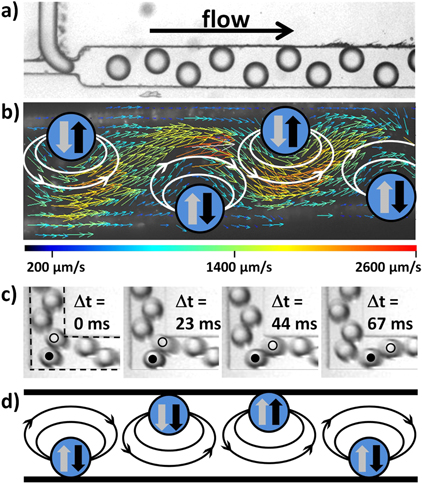
Figure 1. (a) Generation of microfluidic crystals using a step-emulsification geometry. (b) Flow field determined by particle image velocimetry in the lab frame. Note, that for experimental reasons a different device material and emulsion system had to be used for the PIV-experiments as explained in appendix  bend. The boundaries of the bend were indicated in the first image. The droplet marked with a dot is repelled from the corner due to its hydrodynamic image [7, 8] and the trailing droplet marked with a circle is squeezed between the leading droplet and the wall and propelled longitudinally out of the corner. (d) Sketch indicating the dipolar flow fields and the resulting transverse forces in a zigzag arrangement with one defect. The width of the main channel is
  for tiles (a)–(c).
Download figure:
Standard image High-resolution imageComputer simulations were conducted using multi-particle collision dynamics (MPC) [15–18]. In this mesoscopic method, hydrodynamics are fully reproduced through the dynamics of point-like solvent particles, cf appendix  where
where  is the velocity of the droplet relative to the microchannel. Simulation parameters were chosen to match the experimentally observed velocity ratio
  for an isolated droplet. The collective oscillations are modelled by an initial zigzag arrangement of droplets with a given periodicity. Droplet and flow velocities were tuned to give a Reynolds number
  in the range of the experiments. Since MPC includes thermal fluctuations, the Peclet number
  for feasible droplet and flow velocities is significantly smaller than in the experiments. This choice was dictated by a trade-off between numerical stability and computational cost. Although simulating at higher Peclet numbers is expected to reveal differences in the long term behaviour, the influence of thermal diffusion is sufficiently small to expect reliable results for short simulation times, respectively short travel distances of the droplets. Moreover, a broader range of frequencies is excited in the simulations at higher Peclet number which helps to reveal the full dispersion relation of the phonon modes as will be discussed below.
3. Controlled excitation of collective oscillations
The flattened droplets experience a friction with the top and bottom channel wall and thus move slower than the surrounding liquid phase. This leads to a quasi two-dimensional dipolar flow field around each droplet, cf figure 1(b). However, note that only the part of the dipolar field is drawn that is relevant for the effective hydrodynamic forces. The droplets produced by step emulsification self-organize into a stable zigzag configuration, where the forces from the dipolar flow fields from the neighbouring droplets cancel out [6, 13]. When this droplet arrangement is guided around a 90° bend, a defect in the ordering can be achieved, as displayed in figure 1(c). In the resulting droplet arrangement the zigzag symmetry is broken and some droplets experience a net hydrodynamic force which drives them towards the opposite channel wall, see figure 1(d).
The defect in the zigzag symmetry created in this way propagates backwards in the co-moving frame of the droplets (see supplemental movie 1, available at stacks.iop.org/njp/16/063029/mmedia). If the droplet size relative to the channel width is chosen appropriately, defects can be generated periodically. The defects then initiate global sine-waves with well defined wavelength along the droplet train that travel forward in flow direction, see figure 2(a) and supplemental movies 2 and 3. The sine waves are very stable and could be observed without any change for channel lengths up to 10 cm, i.e., for distances more than two orders of magnitude larger than a typical wavelength. The wavelength λ along the droplet train depends on both the droplet size and the droplet spacing, i.e., droplet density. Varying these parameters, various wavelengths can be specifically excited, typically containing 4–9 droplets per wavelength. However, the experimentally accessible wavelength variation is limited to a factor of about three as the size of the droplets and the droplet density have to be chosen such that the droplets are close enough to affect each other by hydrodynamic interactions but do not deform each other in lateral direction by steric contact. The hydrodynamic interactions between droplets are observed to be strongly influenced by the confinement of the droplets, i.e., the degree of flattening and the absolute size of the system. The dense droplet arrangements presented in this paper could not be produced with equally sized droplets confined into channels with just  height instead of the used channel height of 120
  , as in the shallow channels the droplets are strongly repelling each other. For an increased channel height of about
  at similar vertical drop confinement, we even managed to generate a collective droplet oscillation while keeping all droplets in steric contact for all times (see supplemental movie 4). As mentioned above, the droplet friction with the channel walls and thus the relative velocity of the droplets in the continuous phase depends on confinement ratio and linear dimension and influences the strength of the dipole forces. Numerically, we account for the different velocities by using the experimentally determined velocity ratio K.

Figure 2. (a) Travelling sine waves with different wavelength as generated by periodic defects for two different droplet sizes (top) and by numerical simulation (bottom). The width of all microfluidic channels are  . (b) Configuration space trajectory of five neighbouring droplets in the co-moving frame of the droplets as extracted from the experiments. To avoid overlaps, the lateral distance between the trajectories was increased. The trajectories of three time intervals are coloured in red (light grey), blue (dark grey), and green (grey). (c) Sketch of the five droplets from (b) using the same colour code with indicated directions of motion in the co-moving frame of the droplets.
Download figure:
Standard image High-resolution image4. Analysis of collective oscillations
In the following, we analyse and discuss the specific experimental and simulation results for a wavelength of six droplets with radius of  μm and crystal spacing
  μm. The results are equally valid for other wavelengths and the discussion applies to both experiments and simulation unless mentioned otherwise. The motion of five neighbouring droplets in the co-moving frame is plotted in figures 2(b), (c). Due to the transverse confinement in the narrow channel and the longitudinal confinement by the crystal spacing, the space trajectory of each droplet describes a figure-eight and each droplet has a constant phase shift with respect to its neighbouring droplets. The transverse displacement has a comparably large amplitude which is given by the lateral confinement, given by the channel width W and the droplet radius R,
  . This confinement defines the wavelength of the experimentally observed transverse droplet oscillation. Additionally, the flow velocity of the continuous phase across the channel is not homogeneous and is slower at the channel walls as a consequence of the no slip boundary conditions. Thus, the droplets also slow down in the longitudinal direction whenever they approach the channel walls and move backward in the co-moving frame. Similarly, the droplets travel forward in the co-moving frame when crossing the channel. The amplitude of this longitudinal oscillation is given by the crystal lattice, i.e. the droplet spacing a and the droplet radius R,
  , which defines the stable mode in longitudinal direction and which is smaller than the amplitude in transverse direction. Thus, due to the lateral confinement, the transverse oscillation is coupled to a longitudinal oscillation where one full cycle of the longitudinal oscillation is completed while the droplet moves from one wall to the other. However, this droplet movement from one channel wall to the other only corresponds to half a transverse cycle. Accordingly, the constant phase shift between neighbouring droplets differs by a factor of two between transverse and longitudinal modes, i.e.,
  and
and  for the considered wave.
To analyse the droplet oscillations quantitatively, we recorded the droplet positions  for all N droplets labelled by
  and for T data frames obtained every
  . From these we extract the elongations
  and
and  , where
  and
and  is the center of the channel. The elongations were used to calculate the power spectra of the Fourier modes


for the transverse and longitudinal oscillations both from experimental and simulation results. The main feature of the experimentally observed stable mode are distinct peak values for both modes, cf figures 3(a), (b). The maximum of spectral density at the main peaks indicates that the collective oscillation of the droplets is dominated by one specific wavelength. The corresponding phonon spectra obtained from simulations are displayed in figures 3(c), (d). They show a continuous signature revealing the full dispersion relation with a sine-like dependence of the frequency on the wave vector. This complete signature results from the small Peclet number, i.e., from the influence of thermal fluctuations that excite all the phonon modes.
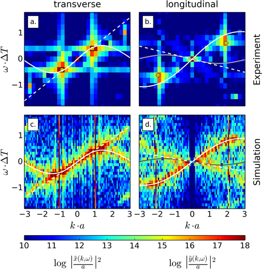
Figure 3. Power spectra of the Fourier transform of the droplet oscillations as extracted from experimental (a), (b) and simulation results (c), (d). (a), (c) Transverse modes  ; the white solid curves denote the prediction for acoustic phonons from the linearized theory (3) for
  whereas the white dashed lines correspond to the continuum approximation with nearest neighbour interactions only. (b), (d) Longitudinal modes
  . The black/grey solid curves are the prediction
  from (4) whereas the dashed lines correspond to the continuum approximation. The white solid curves represent
  and illustrate the coupling of the longitudinal to the transverse modes. The circle symbols mark the main peaks of the experimental spectrum indicating the preferred wave vectors. The time scale is
  .
.
Download figure:
Standard image High-resolution imageA comparison of the experimental and numerical transverse power spectra shows that the dominant frequencies are identical. Moreover, they are in excellent quantitative agreement with the dispersion relation for transverse phonons  predicted by a linearized far-field theory for two-dimensional channel flow [7, 8], cf details of the calculation in appendix


where  , and
, and  . Note that
  in (3) has a slightly different form than reported in [7, 8], as it takes into account all linear-order terms in the expansion, cf appendix
  of the phonon mode along the droplet crystal in the direction of the flow. The dispersion relation is also in agreement with the short wavelength travelling backwards as observed experimentally for a single defect. The quantitative agreement also shows that the linearized far-field hydrodynamic interactions describe the transverse phonon dynamics remarkably well, even though the droplets nearly touch each other [8]. From the experimental findings it even seems that the validity of the far-field approximation for an ensemble of flattened and comparably large droplets is extended to smaller drop distances compared to an ensemble of micro-particles with similar confinement [4, 20].
The observed longitudinal modes are not actively excited and have a smaller amplitude compared to the transverse oscillation, but still show a clear signature especially in the simulation results. The dominant frequencies derived from experimental and simulation result agree quantitatively. Interestingly, however, the longitudinal modes show a dispersion relation that differs from the prediction of the linearized theory, cf figures 3(b), (d) where  from (4) is plotted as a grey line. We observe that the maximum of the longitudinal dispersion relation appears shifted towards
  , and for all k, the longitudinal modes propagate in the flow direction, in contrast to the analytical prediction (4). The observed shape of the longitudinal dispersion relation resembles the scaled shape of the transverse dispersion relation. This apparent resemblance is confirmed by the correlation strength
between longitudinal and transverse modes


The correlation strength is shown in figure 4(a). Whereas acoustic phonons are expected to have high correlation for  [10], we observe high correlation for
  . For small wavelengths the dominant correlation is located around
  . The origin of the longitudinal modes can be explained in terms of the observed figure-eight motion of individual droplets (figure 2). The droplets slow down at both channel walls, i.e., twice during a transverse cycle such that
  . Spatially, a full longitudinal wave extends over each crest or trough of the transverse wave, hence
  . The combination leads to the dispersion relation

which is plotted in figures 3(b), (d) and shows quantitative agreement with the observed longitudinal spectra. We conclude that the longitudinal modes do not originate from direct dipolar interactions between the droplets, but they are a consequence of the inhomogeneity of the imposed flow  which is slower near the lateral walls. The longitudinal motion is hence coupled to the considerable amplitude of the actively excited transverse modes, because the spatial dependence of
  introduces nonlinear terms in the equation of motion.
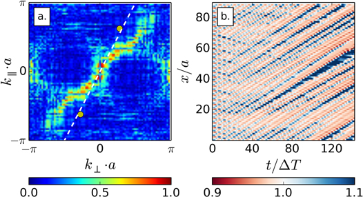
Figure 4. (a) Correlation strength  of longitudinal and transverse phonons as determined from the numerical simulation. The circle symbols mark the dominating wave vectors observed experimentally (extracted from figure 3 the dashed line represents the phenomonelogical dispersion relation
  discussed in the text). (b) Space-time diagram of the longitudinal droplet distance observed in simulation results.
Download figure:
Standard image High-resolution image5. Long-time behaviour and onset of instability
In the numerical power spectra in figures 3(c), (d) a weaker and apparently linear branch is present besides the main branch. The secondary branch is consistent with the faint secondary peaks in the experimental power spectra (figures 3(a), (b)). This branch has a positive slope for transverse modes and a negative slope for longitudinal modes. In the simulation results, the linear branches are relatively weak for short simulation times, as observed experimentally but become more pronounced for longer times, which indicates a relation to the long-time behaviour of the droplets. The space-time diagram of the numerically obtained longitudinal elongations in figure 4(b) reveals the formation of gaps and break-up of the crystal into smaller subunits with time. This is potentially caused by nonlinear interactions between longitudinal and transverse modes, similar to observations for unconfined crystals [8] and in dusty-plasma crystals [21].
A potential explanation for the emergence of the linear branches in the power spectra at longer times is the following: as long as the microfluidic crystal structure remains intact, the longitudinal positions of the droplets oscillate around their 'equilibrium position'  . In the co-moving frame, where the first droplet oscillates around
  , this equilibrium position is just
  , which was already implicitly used in the Fourier transformations (1) and (2). In addition to the oscillatory motion, the droplets may diffuse away from this position over time. It may then be more appropriate to regard the droplet arrangement as a disordered ensemble, which suggests to replace the finite-differences in the equation of motion by their continuum approximations [22, 23]


where  and
and  are the elongations introduced above. Using this continuum approximation to derive the equations of motion and the dispersion relation as in appendix


For small  these expressions coincide with the expansions of (3) and (4), i.e., for small
  a microfluidic crystal and a continuum show the same linearized dispersion. We note yet that the approximation in (9) and (10) demands small differences of the equilibrium positions,
  , and for the relatively strong lateral confinement between neighbouring droplets we study, hydrodynamic interactions are screened such that we can restrict the sum in the dispersion relation to the nearest neighbour interactions j = 1.


These dispersion relations are linear in k and are plotted as dashed lines in figure 3. They match the secondary features reasonably well. Interestingly, this also seems to be the case at the edge of the Brillouin zone, which could be a consequence of short wavelength oscillations in the subunits of the droplet train. In the simulations, these features are more pronounced because the breakup of the crystal is promoted by thermal fluctuations which may trigger instabilities leading to fast growing modes [8]. However, in our experiments, the amplitudes of the longitudinal fluctuations are not growing on the observed length and time scales, hence the secondary peaks remain faint in the experimental power spectra. This experimental observation seems to indicate that oscillations in a dense microfluidic crystal with small droplet spacing are more stable than in a microfluidic crystal with large droplet spacing [5]. A detailed stability analysis is beyond the scope of this work, however, our simulation results suggest that the considered systems of microfluidic droplets are also suited to study the nonlinear mechanisms that lead to instabilities.
6. Summary and conclusion
Using slightly flattened droplets in a quasi two-dimensional microfluidic channel, coupled phonon modes could be experimentally studied in a dense one-dimensional microfluidic crystal and quantitatively compared to simulations and analytical results. The experimentally excited oscillation modes can be selected by the lateral droplet confinement, i.e. the droplets radius and the droplet spacing. Consequently different oscillation modes and wavelength can be controllably excited when adjusting the droplet confinement. The specifically excited transverse oscillations can be described as acoustic phonons by a linearized far-field theory even in a dense system where droplets are in steric contact. A similar behaviour could not be observed in our experiments for disk like droplets, which demonstrates that the hydrodynamic interactions are strongly influenced by the dimensionality of the system. The considerable amplitude of the excited transverse oscillations leads to a nonlinear coupling of longitudinal to transverse modes. The coupling is induced by the lateral variation of the imposed flow across the channel. The coupled longitudinal modes are beyond the existing analytic description, but can be quantitatively described by a phenomenological dispersion relation.
The small longitudinal droplet spacing in the observed dense droplet crystals supports the coupling of the longitudinal and the transverse modes leading to very stable collective oscillations. Dense and laterally confined microfluidic crystals are therefore a promising system to study collective effects and nonlinear phenomena arising from hydrodynamic interactions in crowded environments out of equilibrium and under confinement. Our approach allows to gain insights into the self-organizing mechanisms and can be used to improve the performance of microdroplet applications in various areas [24].
Acknowledgments
The authors would like to thank Tsevi Beatus, Roy Bar-Ziv, Marisol Ripoll and Roland G Winkler for valuable discussions. RS and J-BF gratefully acknowledge financial support by the DFG grant SE 1118/4.
Appendix A.: Particle image velocimetry (PIV)
PIV allows to measure the flow of fluid media. The fluid is seeded with sufficiently small fluorescent tracers who follow the flow without delay. To determine the flow profile PIV does not track individual tracers but, relates on the numerical correlation of a large number of tracers whose position has been changed between two consecutive images (double images) which have been captured within a short time interval [25, 26]. Exposure time and time delay between two consecutive images have to be adjusted to freeze the motion of the tracers and to allow for a reliable correlation of the changed tracer position. In micro-PIV, as used in our experiments, the illumination and the detection is carried out through the same microscope objective. For the experiments presented in the paper we used a commercial micro-PIV setup from LaVision (Germany) with an illumination wavelength of 473 nm and a typical time delay of 10 ms. The measured flow field is presented in figure 1 of the paper as extracted by the commercial software DAVIS (LaVision, Germany) without further image processing.
As commercially available tracers are typically stabilized for an aqueous phase and we were interested in the flow field of the continuous phase, the PIV experiments presented in figure 1 were conducted using an oil in water emulsion. Consequently, the stable generation of monodisperse oil droplets in a surrounding water phase requires a sufficiently hydrophilic device material. Thus, the microfluidic device used for the PIV measurements has the same step geometry and channel dimensions as used for all experiments in the paper but was fabricated from the UV-curable resin NOA83H (Norland Products). The NOA83H device was molded from a PDMS master fabricated by standard soft lithography technologies. The UV curable resin was pre-cured by an uniform UV-illumination for 10 min (wavelength of 365 nm and intensity of 7.5 mW cm ) removed from the PDMS mold and bonded to glass microscopy slides by heating the device for 10 min at 120 °C. Prior to this step, holes were drilled in the glass slides and later connected with plastic tubing connector (Nanoport N-333. Upchurch).
Using this device monodisperse oil droplets (n-hexadecane) were generated in a surrounding aqueous phase containing 2wt% of the surfactant sodium dodecyl sulfate (Sigma) and green fluorescent micro-particles (Thermo Scientific -  ). The typical diameter of the beads is around 1 μm. A suitable concentration of tracers was achieved by diluting 0,64 ml of the original particle solution with 1,65 ml ultra pure water. Flow conditions were similar for all experiments discussed in this article.
Appendix B.: Multi-particle collision dynamics (MPC)
MPC is a mesoscopic simulation method that is capable of reproducing hydrodynamics of a solvent [15, 18]. The solvent is modelled explicitly by idealized point-like particles of mass m. The fluid dynamics emerges from mass, momentum and energy transport in the particle ensemble whose equation of state is that of an ideal gas.
The particle positions and momenta are updated iteratively in successive streaming and collision steps. During the streaming step the particle moves freely

where h is the time between collisions. In the collision step, the particles are sorted into cubic collision cells of size  . In each cell the particles then exchange momentum while the momentum of the collision cell is conserved. In this work, we use a collision rule that also conserves the angular momentum of the cell. In addition, we apply an Anderson-like thermostat to control the temperature. This collision operator is denoted as AT+a in the nomenclature of [27] and updates the particle velocities according to

where  is the centre of mass velocity of the collision cell containing
  particles,
  is the moment of inertia tensor of the particles,
  is the relative particle position, and
  is a random velocity drawn from a Maxwell–Boltzmann distribution. The cell grid is shifted randomly before each collision step to restore Galilean invariance of the system [28]. The dynamic viscosity η of the MPC-AT+a solvent for large number density n (particles per cell) is given by

where  is the imposed temperature and d = 2 is the dimensionality of the system.
The immersed droplets are modelled as rigid discs of radius R that are moved according to Newtonʼs equation of motion. The discs are coupled to the fluid by a no-slip boundary condition. In the streaming step, a bounce-back boundary condition is applied to the solvent particles, i.e.,  where
where  is the boundary velocity. In the collision step, the cell volume occupied by the boundary is filled with virtual particles that are distributed randomly within a layer of width
  . The velocities of the virtual particles are drawn from a Maxwell–Boltzmann distribution and the velocity
  of the boundary is added [16]. The momentum change of the solvent particles during streaming and collisions is accumulated and leads to the boundary force
  that moves the discs [19].
Since hydrodynamics is not resolved on short distances, we add steric droplet-droplet and droplet–wall interactions. These are modelled as Weeks–Chandler–Anderson (WCA) potentials

where  for droplet–droplet interactions, and
  for droplet–wall interactions.
  is the distance of the droplet centres, or the distance of the droplet centre from the wall surface, respectively.
The friction at the top and at the bottom of the Hele–Shaw cell is accounted for by a friction force  where
where  is the velocity of the droplet relative to the microchannel. The flow is driven by an external force
  corresponding to a constant pressure gradient across the channel. The initial setup of the droplets is a triangle wave of a given wavelength λ.
The basic simulation units are chosen such that the size of an MPC collision is  and the MPC time step is
  , where the time scale is
  , and m is the mass of one MPC particle. The parameters for the MPC simulation are the fluid density
  , the driving force
  , and the friction
  . These parameters correspond to a fluid viscosity
  . The mass of the droplets is given by
  . The parameters for the WCA potential are
  and
and  . We varied the channel width W, the droplet spacing a and the initial wavelength λ. The simulation results presented in the main article are for 90 droplets in a channel of length
  and width
  . The initial zigzag pattern was set up with a length of six droplets.
In order to compare the simulation results to the linearized theory and to the experiments, we determined the value  from independent simulation runs with a single droplet under the same confinement. For a channel width of
  we obtained a value of
  which is on the order of the experimental parameters. The oil velocity is in the range
  , such that the Reynolds and Peclet number of the simulations are
  and
and  , respectively.
Appendix C.: Linearized theory and dispersion relations
The complex flow potential for a point-like dipole at position  in the channel evaluated at position
  is [7, 8]
Differentiating  with respect to z we obtain
Note that  is related to the force exerted on other droplets, and it does not contain terms involving the velocity
  or
or  of the droplets.
We expand around  ,
,  ,
,  , and
, and  and keep all linear terms
Now we add the expansion of  around
  and arrive at
Since the expansion of the compressibility factor C around  has a vanishing linear term, we can readily multiply with
  and K, and sum over j to obtain the equations of motion for the nth droplet
Plugging in a plane wave solution we arrive at the dispersion relations


