


Abstract
We investigate the geometric properties of two-dimensional continuous time random walks that are used extensively to model stochastic processes exhibiting anomalous diffusion in a variety of different fields. Using the concept of subordination, we determine exact analytical expressions for the average perimeter and area of the convex hulls for this class of non-Markovian processes. As the convex hull is a simple measure to estimate the home range of animals, our results give analytical estimates for the home range of foraging animals that perform sub-diffusive search strategies such as some Mediterranean seabirds and animals that ambush their prey. We also apply our results to Levy flights where possible.
Export citation and abstract BibTeX RIS

Content from this work may be used under the terms of the Creative Commons Attribution 3.0 licence. Any further distribution of this work must maintain attribution to the author(s) and the title of the work, journal citation and DOI.
GENERAL SCIENTIFIC SUMMARY Introduction and background. Random walks are omnipresent in everyday life. In the often-encountered two-dimensional environment it is desirable to quantify the geometric properties of the area covered by the random walker. A simple and widely employed approach makes use of the convex hull of the trajectory, which is the minimum convex polygon enclosing all points visited during the walk. Nevertheless, convex hulls of Markovian processes such as Brownian motion have only recently been taken into consideration. We go beyond this and examine the geometric properties of continuous time random walks (CTRWs), which are genuinely non-Markovian stochastic processes.
Main results. We derive exact analytical expressions for the time-dependent average perimeter and area of the convex hull of CTRWs, a class of non-Markovian sub-diffusive processes. Such processes are characterized by a sub-linear time dependence of the mean square displacement.
Wider implications. In both experimental and theoretical ecology there is interest in the estimation of the geographic range over which a single or a group of animals forage in order to better plan habitat conservation. Since the motion of many foraging animals is approximately random, the average area of the convex hull enclosing their trajectories can be used as a good estimate of the geographic range. Other applications include determining the spatial extent of an epidemic outbreak among animals and potentially, outside of biology, assessing the area affected by spreading contaminants.
 Figure. An example of the convex hull of planar Brownian motion.
1. Introduction
Random processes such as random walks or Brownian motion are models that describe the diffusive motion of particles whose transport properties are characterized by a linear time dependence of the mean-squared displacement. Whenever a process deviates from this linear dependence it is said to exhibit anomalous diffusion. A model accounting for such anomalous diffusion is the continuous time random walk (CTRW), a random walk where the waiting time between the successive displacements is random [1–3]. Recently the CTRW has been applied to describe anomalous transport in a variety of different complex systems [4–7]. While the bulk of the research focuses on one-dimensional quantities such as the MSD, little is known about two-dimensional properties of CTRWs. It is often desirable, however, to quantify the geometry of the space covered by the sample path of a random process. For example, in ecology one is interested in the estimation of the home range of an animal or a group of animals for habitat conservation planning [8, 9]. For this, one requires information about the geometry of the home range and how it evolves in time. Since the motion of many foraging animals is approximately random, in this field one is naturally interested in the geometric properties of two-dimensional stochastic processes [10–12].
A simple and widely employed approach to quantify the area covered by a random two-dimensional motion is the concept of convex hulls. The convex hull of a set of points in the plane is defined as the minimum convex polygon that encloses all of them (figure 1). If a random set of points or a trajectory of a stochastic process is considered, the corresponding convex hull is also a random quantity and one is interested in the quantities such as the mean perimeter or the mean area of an ensemble of these random convex hulls. While the calculation of properties of a convex hull of uncorrelated random points is quite an old problem, much effort has recently been put into the investigation of the convex hull of one or more Brownian motions and Lévy flights [13]. In the context of branching Brownian motion, convex hulls have been proposed as a way to characterize the spatial extent of epidemics in animals at the outbreak stage [14].
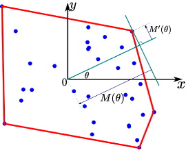
Figure 1. Convex hull of a set of randomly distributed points. M(θ) is the support function and M'(θ) its derivative.
Download figure:
Standard image High-resolution imageThe purpose of this paper is to present an analysis of the random convex hull of a CTRW in the plane. To this end we determine analytical expressions for the time evolution of the average perimeter and area of convex hulls of such processes. It is important to note that, except for the degenerate case of a fixed waiting time, the CTRW is only a Markovian process if the waiting time between the displacements are exponentially distributed. Here we focus on the case of a heavy-tailed waiting time distribution with an infinite mean. Thus for the first time we provide analytical calculations for the convex hull of a class of genuinely non-Markovian processes. Our results can be applied to model the home range of foraging animals that perform a saltatory, intermittent search strategy for their prey. Such an intermittent locomotion can be advantageous for a variety of reasons. The pausing times between displacements help animals recover from fatigue, search more accurately for prey and evade predators more efficiently [15]. For example, rattlesnakes remain in the same position for extended periods of time waiting to ambush a potential prey [16]. Furthermore, there is growing evidence that human activity is drastically changing the foraging habits of animals, forcing them to adopt subdiffusive search strategies. An example for such an induced change of a behavioural pattern is the effects of human fishing on seabirds such as the Balearic shearwater and the Cory's shearwater in the Mediterranean [17]. Due to the presence of trawlers these birds start showing strong site fidelity to certain foraging areas, thus making the overall foraging process subdiffusive. Since the CTRW is a model of diffusion with trapping events, our considerations are also of interest in the context of ground water pollution in porous layers where the diffusion is known to be anomalous [7].
2. Subordinated Brownian motion
A simple random walk in one dimension is characterized by a sequence of jumps of random length λ. For the sake of simplicity, we assume that the jump lengths are independent identically distributed random variables sampled from a symmetric distribution function φ(λ) with finite variance. We shall use pn(x) to denote the probability of finding a random walker in position x = λ1 + λ2 + ··· + λn exactly after n jumps.
As mentioned already in the introduction, the CTRW is a generalization of the random walk whereby random waiting times {τ} are assumed to take place between the random jumps. In order to preserve causality, the {τ} have to be greater than zero. Furthermore, we assume the waiting times to be independent identically distributed positive random variables sampled from a distribution ψ(τ) that is independent of φ(λ). In that case, the probability of finding the random walker at x after a time t is given by  . Here Kn(t) denotes the probability that exactly n jumps occurred up to the time t which reads in the Laplace domain
  , where Ψ(τ) is the survival function denoting the probability that no jump occurs up to time τ [2, 3]. Here and in the following
  denotes the Laplace transform.
The function Kn(t) can be considered as the kernel of a transform that maps a probability density from the domain of an operational time n to that of the physical time t. In the mathematical literature one refers to the random walk x(n) as the parent process and the CTRW as the process x(t) = x[n(t)] subordinated to x(n).
In this paper, we consider the scaling limit of the CTRW which is called subordinated Brownian motion. Since Brownian motion is equivalent to the diffusive limit of a random walk, the series representation of the CTRW shown above has to be substituted, using proper scaling relations, by an integral form [18]. Here we use an intuitive, albeit not so formal, approach introduced by Fogedby [19]. He considered the scaling limit of a CTRW via a set of coupled Langevin equations of the form

where ξ(s) and η(s) are the random noise sources independent of each other and s the continuous equivalent of the operational time n which is sometimes referred to as internal time. Under these circumstances, the equation on the left in (1) is the parent process and the one on the right relates the physical time to the operational time. Analogous to the discrete case, the values of η have to be strictly positive in order to ensure causality. Furthermore, the continuous equivalent of the kernel function Kn(t), defined as K(s,t), is the probability density associated with s(t), the inverse of the stochastic process t(s). For this reason, the existence of s(t) is essential, in which case t(s) must be a non-decreasing right-continuous function.
It can be shown that the set of coupled Langevin equations (1) leads to a time-fractional diffusion equation if the random variable η is sampled from a heavy-tailed probability density such as the one-sided α-stable distribution and if ξ(s) is assumed to be white noise [19]. In other words, if we choose a waiting time probability density with asymptotic behaviour ψ(η) ∼ αbαη−1−α/Γ(1 − α) where 0 < α < 1 and assume x(s) to be a Wiener process, then the resulting stochastic process x(t) in the physical time domain that emerges from (1) is non-Markovian and sub-diffusive. Note that bα is a constant with units [bα] = [Tαt] in physical time t.
In the Laplace domain the waiting time distribution has the asymptotic behaviour  so that in the scaling limit one obtains
  , where cα = bα × r with the constant r being the number of steps per unit operational time [19]. We therefore have [cα] = [Tαt]/[Ts]. Laplace inversion then yields [18, 20]

where Lα(t) is the one-sided Levy-stable distribution with stability parameter 0 < α < 1 whose Laplace transform is given by  [21].
[21].
Combining the distributions corresponding to the two processes x(s) and s(t), i.e. p(x,s) and Kα(s,t), respectively, we can eliminate the internal time to finally obtain the propagator for the subordinated process:

This result is central to subordination theory and will be used frequently in the following. Note that pα(x,t) can be considered as the solution of a non-Markovian diffusion equation, connected to its standard Markovian counterpart, p(x,s), through (3). This equation is valid in general as long as the two functions in the integrand remain non-negative [22].
3. Random convex hulls
Random convex hulls, which are defined as the minimum convex polygons enclosing a set of random points, have attracted much interest in the last 50 years and there is an ongoing effort to determine the statistical properties of convex hulls associated with a variety of different planar random processes. For Brownian motion it is possible to analytically evaluate the average perimeter length and the average area of the random convex hull (for a review see [23]).
Since the focus of this paper is on the properties of convex hulls of CTRW processes, we shall shortly summarize some important results of the theory of random hulls which are especially well suited to treat correlated stochastic processes. It is known that the perimeter L(T) and area A(T) of the convex hull of a single path can be determined using the Cauchy functionals [13, 23]

and

where M(θ), which is referred to as the support function, is the maximum extent of the projection of the given stochastic path in the direction of the angle θ∈[0,2π]. For any planar stochastic path (x(t),y(t)) in continuous time t∈[0,T] the support function has the form

Figure 1 gives a geometric interpretation of the support function and its derivative. A concise derivation of these results is provided in [23].
4. Convex hulls of continuous time random walks
We shall now proceed to calculate the properties of the random convex hull enclosing the stochastic path r(t) = (x(t),y(t)) traced by a CTRW in the xy plane in the time interval 0 < t < T. In order to calculate the average perimeter and area of such a process, we have to determine the support function associated with it. As shown in (6), the support function depends on the angle θ with respect to the x-axis and an arbitrarily chosen origin, for which we will use the starting point of the stochastic process.
With (6) in mind, we introduce zθ(t) = x(t)cos θ + y(t)sin θ so that the support function can be written as ![$M(\theta )=\max _{t\in [0,T]}\{z_\theta (t)\}$](https://content.cld.iop.org/journals/1367-2630/15/6/063034/revision1/nj470774ieqn7.gif) . Furthermore, let us denote hθ(t) to be the derivative of zθ(t) with respect to θ. At some point within the time interval [0,T] the planar CTRW will reach its maximum excursion in the direction θ. Let us denote this time with τm and use ρα(τm,T) for the corresponding probability density function. The support function and its derivative can then be written as
. Furthermore, let us denote hθ(t) to be the derivative of zθ(t) with respect to θ. At some point within the time interval [0,T] the planar CTRW will reach its maximum excursion in the direction θ. Let us denote this time with τm and use ρα(τm,T) for the corresponding probability density function. The support function and its derivative can then be written as


The quantity M'(θ) gives the value of the projection of the planar CTRW onto the direction perpendicular to θ attained at time τm. In the particular case where θ = 0, we have that z0(t) = x(t) and h0(t) = y(t) so that the support function reduces to M(0) = z0(τm) = xm while its derivative is given by M'(0) = h0(τm) = ym.
Calculating the distributions of the hull perimeter L(T) and area A(T) is very difficult in the Brownian case, let alone for CTRWs. Therefore, in this paper we settle with the task of calculating the average values of these quantities. Since we neglect any external biases, the process under consideration is isotropic in space. Thus, we can take θ to be zero without loss of generality, and write down the expressions for the average perimeter and area, respectively as

and

where 〈·〉 denotes an ensemble average.
According to (9), the average perimeter of the convex hull of a planar CTRW can be determined using the average maximum excursion of the one-dimensional stochastic process z0(t) in the interval [0,T]. Hence we need to calculate the density function fα(xm,T) for the maximum positive-valued excursion of the process z0(t). In the case of Brownian motion, it is well known that the probability density of the maximum positive excursion from the origin achieved in the time interval [0,S] is given by Feller [24]  , where D = r〈λ2〉/2 is the diffusion constant of the underlying Brownian motion with units [D] = [L2]/[Ts]. This result, together with the subordination concept can be employed to calculate the maximum excursion density fα(xm,T) of a CTRW in the physical time T. Substituting f(xm,S) into (3) one obtains

Laplace transforming (11) yields  , where ν = α/2 and
  . Back transformation then provides the distribution of the maximum

which, for D = 1, confirms the result obtained by Schehr and Le Doussal [25] with the real-space renormalization group method. This result was also obtained by Carmi et al [26] using functionals of sub-diffusive CTRWs.
Having the analytical expression for fα(xm,T), the first moment 〈xm(T;α)〉 can be calculated (see 3.6 of [3]) and we obtain for the average perimeter of a planar CTRW

where Dα = D/cα is the generalized diffusion constant with units [Dα] = [L2]/[Tαt].
The determination of the average area of the convex hull of a planar CTRW is slightly more involved. From (10) it is apparent that we need to calculate the moments 〈x2m〉 and 〈y2m〉. While 〈x2m〉 can be extracted directly from the probability density function (12), giving

the calculation of 〈y2m〉 is not so straightforward. In principle, we need to know gα(ym,T) i.e. the probability density of the value of y(τm) attained at the instance when the process x(τm) reaches its maximum excursion in the positive direction in the time interval [0,T]. However, the difficulties of calculating gα(ym,T) arise due to the fact that the two one-dimensional projections x(t) and y(t) of the two-dimensional CTRW are not independent. In contrast to the Markovian case, when a planar CTRW is projected onto the x and y directions, there always remains a correlation in the time of the 'jumps'. The two one-dimensional projections always change direction simultaneously, no matter how the decomposition is done.
The way around this problem is again to use subordination. Therefore, we note that the parent process can be decomposed into two independent one-dimensional Brownian motions. The trick is then to subordinate these two processes to the same subordinator, i.e. we have to consider the Langevin system

where ξx(s) and ξy(s) are two independent realizations of the same white noise source and η(s) is chosen as before.
On their own, the first two equations in (15) constitute a planar Brownian motion whose two components x(s) and y(s) are independent and are governed by the same propagator p(·,s). Therefore, in operational time it is legitimate to express the probability density governing the random variable ym as

where σm∈[0,S] is the time when the process x(s) reaches its maximum whose probability density ρ(σm,S) = [σm(S − σm)]−1/2/π is given by the famous arcsine law [24], and p(y,s) is the propagator associated with y(s). It is important to observe that such a decomposition of g is not possible for the CTRW, due to the correlations between x(t) and y(t) in the physical time t.
By linking the probability density functions governing ym in the two time domains we are now able to determine g(ym,T). Substituting g(ym,S) into (3), one obtains

Having this equation in mind, the formal expression for the second moment of the random variable ym in the physical time domain is given by

The easiest way to simplify this expression is to integrate first with respect to ym, which amounts to 〈y2(σm)〉 = 2Dσm. Performing the integration over σm one obtains

where we have used the expression in (2) for Kα. Finally, by substituting the last two results into (10), one obtains as the second central result of this paper for the average area of the convex hull of a CTRW

One might argue that the results in (13) and (20) could have been obtained by applying the subordination transformation directly to the mean perimeter and area relative to the Brownian case. However, when dealing with the subordination method, the only way to be sure of obtaining meaningful results is to work with probability densities [22].
To verify our analytical results (13) and (20), we have performed numerical simulations. To this end, an ensemble of two-dimensional CTRWs was created and the convex hulls around them were constructed using a standard algorithm known as the Graham scan [27]. Figure 2 shows a perfect agreement of the analytical results with the simulations.
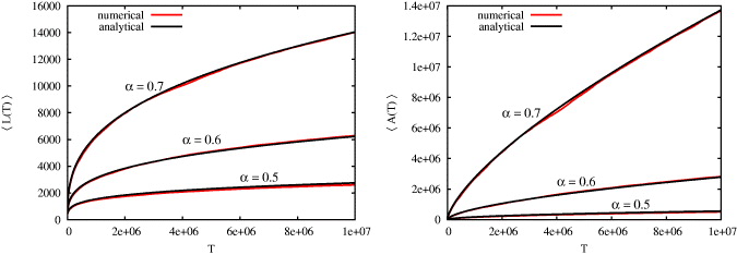
Figure 2. Time evolution of the average perimeter (bottom panel) and area (top panel) of the convex hull around a CTRW for different values of α. We observe a perfect agreement of the analytical results (13) and (20) and the numerical simulations.
Download figure:
Standard image High-resolution image5. Subordinated Lévy flights
So far we only considered the case where the distribution of the displacements has a finite variance. Some of the results, however, can be generalized to the case of Lévy flights that are characterized by a heavy-tailed jump distribution of the form φ(λ) ∼ Bμ/|λ|1+μ, where Bμ is a constant. In particular, we will consider jump distributions whose characteristic function has the form  . For 1 < μ < 2 this distribution has a finite mean but a diverging variance and the Lévy flight exhibits super-diffusive behaviour. On the other hand, μ = 2 recovers the Gaussian distribution with standard deviation
  .
.
According to (4), in order to calculate the mean perimeter of a subordinated Lévy flight we need to know the mean value of the maximum excursion of the corresponding one-dimensional process which is given by

where fμ(xm,S) is the probability density of the maximum excursion of a Lévy flight after time S. At first glance this imposes a problem since, to the best of our knowledge, the exact expression for fμ(xm,S) is not known. However, the leading order behaviour of the mean maximum 〈xm(S;μ)〉 of a Lévy flight after S steps can be alternatively obtained by employing an asymptotic expansion of the Pollaczek–Spitzer formula as was shown by Comtet and Majumdar in [28]. They obtained

where Dμ = aμr is the generalized diffusion coefficient of Lévy flights in operational time with units [Dμ] = [Lμ]/[Ts] and a1/μμ the scale parameter of the jump distribution. Since averaging is a linear operation we can exchange the orders of integration in (21) yielding

Observe that a similar expression has recently been obtained in [29]. Inserting (22) into (23) and applying (4), we finally obtain for the mean perimeter of a subordinated Lévy flight

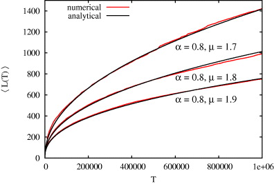
In this case we also find excellent agreement between the analytical results and the simulations (see figure 3). Moreover, the result in (24) reduces to (13) for μ = 2 as it should. Note that in the Gaussian case D = σ2r/2 and that  when μ = 2.
Figure 3. Time evolution of the average perimeter of a subordinated Lévy flight for α = 0.6 and three different values of the stability parameters μ. The simulations agree well with the analytical solution (24).
Download figure:
Standard image High-resolution image
The average area of the convex hull of a subordinated Lévy flight is divergent since already the mean-squared displacement of a Lévy flight diverges, i.e. 〈x2(t)〉 = ∞ for all times.
It is well known that a Lévy flight can also be obtained by subordination of a normal random walk [30]. Therefore, our method works, in principle, also for Lévy flights without resorting to the results of [28] for the mean maximum excursion. The subordination method yields the correct scaling behaviour for the mean perimeter of the convex hull, but it interestingly overestimates the pre-factor. This discrepancy is due to an underestimation of the maximum distribution near its peak at zero, while the tail behaviour of the maximum distribution is accounted for correctly by the subordination method. An intuitive explanation can be given by noticing that the subordinated Lévy flight is obtained by sampling points from a Brownian trajectory at irregularly spaced time intervals that are distributed according to a broad-tailed inverse power law. The presence of large sampling intervals implies that it is relatively likely that the underlying Brownian motion will make small excursions above zero that will be completely missed by the sampling procedure.
6. Conclusion
In this paper, we have considered two-dimensional properties of anomalous diffusion processes. Based on the method of subordination, we have analytically calculated the mean perimeter and average area of the convex hull for a class of non-Markovian processes. The analytical results were found to agree perfectly with numerical simulations. For the mean perimeter, we generalized our results to the case of subordinated Lévy flights. Thus for the first time we obtained two-dimensional geometric properties of CTRW processes.
Keeping in mind the broad range of disciplines, where the CTRW is employed as a stochastic model, our findings are valuable whenever information about the area or the perimeter of such a two-dimensional process is of interest.
Acknowledgments
Mirko Luković acknowledges the scholarship granted by the IMPRS-pbcs.