


Abstract
Although the electromagnetic resonances of individual nanostructures can be studied by electron or photon interactions alone, exciting new possibilities open up through the simultaneous use of both. In photon-induced near-field electron microscopy (PINEM), for example, single nanostructures are optically excited by short, intense pulses and concurrently imaged with high spatial resolution by fast electrons, which act as negligible probes of electric fields. Controlling their relative arrival time provides access to the dynamics of the electromagnetic response in the near field by recording images of the electron energy loss (or gain) spectra. In this paper, we investigate the transition from optically dominated PINEM to conventional, electron-dominated electron energy-loss spectroscopy (EELS). During the systematic reduction of optical excitation intensity to zero, a novel electro-optical interference effect emerges. It reveals itself at those optical field strengths that lead to prominently visible constructive and destructive interference patterns of the optical and electron radiation fields which are scattered by a nanostructure. The interference patterns reported here allow one to achieve higher temporal, energy and spatial resolutions of the modal dynamics in electron microscopy.
Export citation and abstract BibTeX RIS

Content from this work may be used under the terms of the Creative Commons Attribution 3.0 licence. Any further distribution of this work must maintain attribution to the author(s) and the title of the work, journal citation and DOI.
GENERAL SCIENTIFIC SUMMARY Introduction and background. On the one hand, photon-induced near-field electron microscopy is a powerful time-resolved technique for investigating the optical density of states. Within this method generated electron pulses of sub-picosecond duration are used as probes of the optically induced modes of structures, while the structure is excited with sub-picosecond optical pulses at high intensities. On the other hand, electron energy-loss spectroscopy is based on the interaction of the electrons with the electromagnetic field scattered by the sample, due to the electron impact. Here, using a numerical approach, we study the interplay between these two methods by systematically investigating the effect of the intensity of the incident laser field.
Main results. Depending on the intensity of the laser fields, either photon-induced or electron-induced processes can be dominant. At an intermediate intensity, both contributions are important and interference fringes become visible in the time–energy map, which is clear evidence of constructive and destructive interferences of the scattered photons due to the electron- and photon-induced polarizations. This phenomenon is only visible for sub-femtosecond longitudinal broadening of the electron pulse.
Wider implications. The interference fringes observed at intermediate intensities of the laser field can be used for investigating the plasmonic modes of single nanoparticles with high temporal, energy and spatial resolution. Moreover, the visibility of the interference fringes can be an estimate of the mutual coherency of the incident electrons and photons.
 Figure. Computed electron energy-loss spectra versus delay and energy loss, at different incident peak laser intensities, for a gold nanoprism with edge length of 400 nm and a height of 40 nm, on top of a Si3N4 substrate of 30 nm thickness. The longitudinal broadening of the electron wave function is 10 nm, and the carrier kinematic energy is 200 keV. The temporal broadening of the optical pulse is 10 fs.
1. Introduction
Microscopy of the electromagnetic modes in optical systems with high spatial resolution has been achieved using electron energy-loss spectroscopy (EELS) [1–5]. Electron microscopy benefits from the very short de Broglie wavelengths of the moving electrons in comparison with the large wavelength of incident photons in optical microscopes, which allows resolving nm-scaled features of the investigated structures. Although the electron probe size in this technique can be even in the sub-nanometer range, the interaction volume is typically larger due to long-range Coulomb forces. This so-called Coulomb delocalization [6, 7] depends on the magnitude of the energy loss suffered by the electron. Its value is approximately 8 nm at 3 eV energy loss and further degrades at lower losses [6], becoming comparable with the spatial resolution of other microscopy techniques [8]. However, interaction of moving electrons with the optical modes of the system obeys specific selection rules other than optical excitation. Electrons can also interact with optically dark modes of the sample [7, 9, 10]. Moreover, they may excite longitudinal currents in the specimens which occur in radiation-free modes such as toroidal moments [3], which cannot be excited with far-field optical excitations.
Recently, by introducing sub-picosecond pulsed electron sources in combination with laser pulses of similar duration into the electron microscopes, it became possible to investigate the temporal behavior of electromagnetic modes of nanostructures [11–16]. Using this method, known as photon-induced near-field electron microscopy (PINEM), the dynamics of excited modes in phase space (frequency–time space) was demonstrated [11]. In this technique, an external optical pump of high intensity is used to excite certain modes of the structure, while the pulsed electrons are used as probes. The temporal evolution of the optical modes is imaged for a fixed delay between the intense optical pump and the electron probe [17]. However, the achievable temporal resolution of this technique is limited by the broadening of the pulsed electron source. Recently, femtosecond electron pulses have been designed by utilizing metallic nanotips [18–21]. The huge field enhancement occurring at such tips exposed to optical pulses can result in higher-order photon-induced electron emission due to the optical nonlinearity of the metals. This can be used to achieve electron femtosecond pulses even without the application of a bias voltage [18]. Furthermore, in order to compress electron pulses of femtosecond duration into the attosecond regime, usage of spatially dependent ponderomotive forces has been proposed [22–25]. Simulations have shown that by introducing an optical grating composed of two counter propagating waves of different frequencies, it is possible to compress electron pulses of 300 fs into trains of only 15 as electron pulses [23].
It is well known that the polarization of the incident optical field within the context of PINEM plays an important role in decomposing the symmetry of the modes of the structure that are excitable with far-field radiation. However, dark modes and radiation-free modes of the structure are not detectable with this technique, since the intensity of the laser beam is so high that it dominates the overall response of the structure in such a way that the relatively weak response of the structure to electrons could be neglected in previous reports [13, 26, 27]. In the range of low laser intensities, a systematic study of the effect of the intensity of the laser field on the recorded PINEM data is still lacking. Decreasing the laser intensity shifts the physical situation continuously out of the PINEM and into the EELS regime. At intermediate laser intensities, we can expect a range where the benefits of both conventional EELS and state-of-the-art PINEM are present: While EELS can be used to record all the near-field resonances of the structure which exhibit a non-vanishing component of the electric field along the direction of the electron velocity, such as toroidal and dark modes, the laser field can be used as a temporal gate to provide the temporal resolution. The aim of this paper is to numerically investigate this transition range with a special focus on electron–photon interference effects. Within this transition range a field of microscopy could be performed allowing for high temporal, high spatial and high energy resolution.
Interaction of swift electrons with the electromagnetic modes of the structure and computation of the energy loss suffered by the electrons has been discussed in several publications. Broadly speaking, these reports may be classified into quantum mechanical [26, 28–30] and classical electrodynamics treatments [31, 32]. While the combination of Maxwell and Lorentz force equations can be used to compute the total energy loss suffered by the moving electrons at classical electrodynamics, definition of the energy-loss probability in the context of classical electrodynamics is not straightforward. An attempt to define the energy-loss spectrum in this direction has led to a linear relation between the energy-loss probability and the temporal and spatial Fourier-transformed electric field [2], which is a complex value.
Another type of theoretical treatment of the energy-loss probability is the quantum mechanical approach within the context of semi-classical electrodynamics [26–28, 30]. All of these results show a relation between the energy-loss probability and the intensity of the electric field [30]. In the semi-classical treatment the interaction Hamiltonian is related to the electromagnetic vector potential, which can be computed using Maxwell's equations. A full and concise approach to compute the PINEM results has been provided in [26].
In order to compute the energy-loss probability, we utilize the finite-difference-time-domain (FDTD) method with an electron source incorporated. In addition, optical pulses of arbitrary duration are introduced. Concise attention will be paid to the range of laser intensities which are comparable to that of the scattered field resulting from the incident electrons. We treat the problem using the same semi-classical approach as [26]. Moreover, the behavior of the structure upon the two excitations can be treated in a superposition approach [33]. Specifically, only two simulations need to be carried out regarding each impact parameter of the moving electrons: one simulation for the incident laser field and another one for the incident electrons. Within the context of the non-recoil approximation, the energy-loss spectrum for every intensity and delay of the incident laser field can be calculated using just the results obtained by the mentioned simulations. Details of the method utilized here are discussed in section 2. The results of the simulations using the mentioned approach are presented in section 3, including also discussions regarding the transition from normal EELS to PINEM spectrum in the phase (time–energy) space. Finally, the conclusion will be summarized in section 4.
2. Method
In order to compute the EELS spectra using the FDTD method, a relativistic electron source has been implemented [33]. Instead of modeling the electron source as a singularity, a cloud of charge distribution density will be considered. The spatial extent of this cloud is estimated by the Coulomb delocalization [6, 7]. This approach is equivalent to the interpolation schemes exploited in particle simulations of plasmas [34], in which computational efficiency and accuracy suggest the usage of clouds rather than singular points for charge distributions. Moreover, this assumption is in agreement with the experimentally expected spatial resolution of EELS at low energy losses [6]. The optical source is implemented as an oscillating plane composed of Huygens point sources in the far field (here 1.5 μm above the structure), as shown in figure 1(b).

Figure 1. (a) A single triangular metallic nanoprism positioned upon a substrate, illuminated by electron and photon sources, and (b) the corresponding FDTD simulation domain in which the electron radiation is modeled by the moving cloud of a charge at relativistic velocity and the optical incident pulse is modeled by an oscillating plane composed of Huygens point sources. τ is the delay between the electrons and the photons computed at the top surface of the structure.
Download figure:
Standard image High-resolution imageThe charge density assigned to the electron source in the rest frame of the electron is given by  in which (x0 ,y0 ,z0 ) is the position of the electron, q is the electron charge, and δ ( ⋅ ) is the Dirac delta function. In the laboratory reference frame, within the framework of the non-recoil approximation [2], the charge-density distribution function for an electron moving along the z-axis with the velocity
  will be given by

in which (z',t') are the spatial and temporal coordinate parameters in the laboratory frame, and  is the Lorentz factor. Note that (x',y') = (x,y) . According to Ampere's law, the current source associated with the moving charge distribution function is given by
in which  . It is obvious from equation (2) that the delta function can be approximated by the limit of the Gaussian function.
The Gaussian function introduced in equation (2) allows a direct comparison of the classical electron source with the current density functions obtained from the Schrödinger equation. In order to show that, we first consider an initial Gaussian wave function for the electron source in the laboratory frame as [26]
in which Wxy is the spatial transverse broadening of the electron source which can be approximated by 8 nm, which is the spatial resolution of the EELS in the energy-loss range of interest. The reason why the spatial resolution is larger than the probe size (<1 nm) is the Coulomb delocalization, which is not explicitly considered in our simulations. Therefore the wide focus point used in our simulation mimics the practical resolution of EELS. W'z is the broadening of the electron pulse along the z-axis. Its value is assumed to be 10 nm here, which corresponds to an electron pulse of 48 as duration.  is the electron impact parameter and z0 (t) is the time-dependent position of the electron source.
  and
and  are the electron angular and spatial frequencies. Using the continuity equation
  one can obtain for the current density function
since  in which m0 is the electron mass. By comparing (2) and (4) one can define a relativistic correction for the wave function by setting
  and W'z = Wz /γ .
The evanescent source of radiation which accompanies electrons moving at a relativistic speed is a wide-band source that can excite modes of various energies with their corresponding momenta lying outside the light cone. By introducing a laser source, the scattered field of the laser also sustains photons of certain energies, which are interactively scattered by the electron, within the limit of energy–momentum conservation. In a semi-classical approach, and considering only inelastic scattering, the probability that the electron loses or absorbs a quantum ℏ ω of energy is exactly the same, thanks to the Hermitian interaction Hamiltonian (the electromagnetic vector potential A). The probability that the electron loses or gains energy from n photon quanta is given by [26, 28]

where q is the electron charge and ℏ is Planck's constant, Ws is the temporal broadening of the optical Gaussian pulse, τ is the time delay between the electron and optical pulses and gi (z) is the one-dimensional initial wave function of the incident electron at the electron frame, given by
and Fz is the PINEM field described as [26, 30]
where V is the velocity of the electrons and  is the temporal Fourier transform of the electric field, defined as
  . Correspondingly,
  is the double Fourier transform of the electric field, which corresponds to the fields in (ω ,kz ) space.
  determines the electron impact parameter in the xy plane. In the weak interaction regime, when
 , and for the case of a single plane wave electron source, one can use the asymptotic form of the Bessel function to obtain the probability that the electron loses a quantum of photon energy [30] as
  . By explicitly considering the total electric field as the superposition of the scattered fields caused by the electron radiation and optical sources, the probability is given by
where τ is the temporal delay of the optical pulse with respect to the electron source and A is a positive factor used to scale the amplitude of  , setting the relative importance of the optical versus the electronic contribution to the total excitation. The first term on the right-hand side of the above equation is the energy-loss spectrum when there is no laser field, whereas the second term is the electron-energy gain spectrum [30], and the third term is a correlation function that is related to the experienced phase shift of the electron wave packet, relative to the phase of the incoming light. The third term can be significant only if the intensity of the incoming light is similar to the intensity of the scattered field of the electron source. Clearly, this term contains information about the phase of the PINEM field. Before proceeding, we mention that in the weak interaction regime, the recorded PINEM data are similar to the data measured by square-law optical detectors. Well-known optical spectrographic, tomographic and interference techniques [35–38] can be exploited here in much the same fashion to provide a full characterization of the intensity and phase of the electric field.
3. Results and discussion
In order to verify our method, we first consider the case of a triangular free standing silver nanoprism for which the EELS spectra (when there is no optical radiation) have been computed using discrete dipole approximation [39] and a rigorous boundary element method [5]. The edge length of the nanoprism is 80 nm and its thickness is 10 nm. In our FDTD simulations, the permittivity of the silver is modeled by fitting a Drude model in addition to two critical point functions [40, 41] to the experimental data reported in [42]. The electron energy is E0 = 100 keV. The EELS spectra obtained using the FDTD method are shown in figure 2. They are in good agreement with the results obtained using the semi-analytical methods [5, 39].
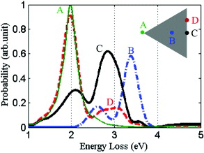
Figure 2. Calculated EELS spectra for a self-supported silver nanoprism with 80 nm edge length and 10 nm thickness. The electron energy is 100 keV and its different trajectories are depicted in the inset.
Download figure:
Standard image High-resolution imageThe structure investigated in this paper is a triangular gold nanoprism with an edge length of 400 nm and a height of 40 nm, on top of a Si3N4 substrate of 30 nm thickness. This structure has been experimentally analyzed using energy-filtered transmission electron microscopy in the Zeiss SESAM microscope [4]. When the only source of radiation is the moving electron, the EELS spectrum can be computed using the first term of equation (8). Using the FDTD method, we computed the energy-loss spectra for the electron sources with different impact parameters (figure 3). The electron energy is taken as 200 keV. Four distinct modes at E = 0.25, 1.00, 1.50 and 1.70 eV are observed, which are due to localized surface plasmon resonances captured inside the material, forming a nano-resonator. The computed resonance energies are in excellent agreement with the measured ones reported in [4]. It should be mentioned that the strong peak at zero energy loss masks the plasmon peak at E = 0.25 eV in the experimental data. However, due to the broad plasmonic resonance, the tail of this mode becomes dominant at E = 0.9 eV, and the acquired image could still visualize the intensity profile for this mode.

Figure 3. Calculated energy-loss probability for a 200 keV electron source traveling at different positions shown in the insets and perpendicular to a triangular gold nanoprism (edge length 400 nm and thickness 40 nm), positioned on top of a Si3N4 substrate of 30 nm thickness.
Download figure:
Standard image High-resolution imageBy gradually increasing the amplitude of the incident laser field from A = 0 to high values, the interaction of the electron with photons changes from a weak-interaction to a strong-interaction regime. Figure 4 shows the energy dependence of the probability for electrons to lose a quantum of photon energy, at different optical intensities, for two values of delay: τ = 0 and  . A central energy of 0.97 eV and a polarization along the y-axis are considered for the incident optical field. For the temporal variation of the optical beam, a Gaussian function with a temporal duration of 10 fs is assumed. For the spatial distribution, a Gaussian profile with a waist of 1.5 μm is introduced. The electron trajectory is assumed to be that of position (a) depicted in figure 3. While the electron source can excite different modes of the structure, the intense laser field centered at the excitation energy of 0.97 eV selectively excites the specific resonance centered at that energy, due to its limited energy broadening and polarization. Most importantly, at intensities of the optical beam in between the weak- and strong-interaction regimes, the third term of equation (8) becomes dominant. At τ = 0 (figure 4(a)) the scattered field caused by the electron shows constructive interference with that of the photons, while at
  (figure 4(b)) destructive interference is obvious due to the fast variation of the phase of the laser field, different from that of the electrons. The interference pattern is obtained for peak areal intensities in the optical excitation field between Ip = 2.4 and 120 MW cm−2. It is noteworthy that this is the range of laser peak powers in which the dominant PINEM field is the single-photon absorption/emission process, as is obvious from figure 16 of [26]. Moreover, this range of powers which can be used for interference microscopy has not been experimentally investigated yet (figure 16 of [26], top). Due to the small bandwidth of the optical pulse introduced here (only 0.07 eV), only a single resonance of the structure at E = 1 eV is excited, and the interference fringes are only obvious in the time domain.

Figure 4. Dynamics of the electron energy-loss spectrum for the electron trajectory as shown in figure 3(a), as a function of laser peak intensity, for two different temporal delays of (a)  and (b)
  between the electron and laser sources. The laser central energy is at E = 0.97 eV and the temporal duration is 10 fs. The color bar is in arbitrary linear units.
Download figure:
Standard image High-resolution imageFigure 5 shows the EELS spectra for the case of only one photon absorption in time–energy space. Exploration of the time domain has been achieved by changing the delay of the optical beam with respect to the electron source. The reference time is taken at  , which is the estimated arrival time for the incident photons.
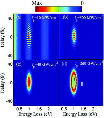
Figure 5. Calculated electron energy-loss probability for the electron trajectory as shown in figure 3(a) versus laser delay for peak laser intensities of (a) Ip = 10 MW cm−2, (b) Ip = 500 MW cm−2, (c) Ip = 40 GW cm−2 and (d) Ip = 260 GW cm−2. The interference fringes at lower laser intensities are related to the dynamics of gaining and losing photons from both the laser field and the scattered field of the electrons, while at higher intensities only the optical field is dominant. Region (I) shown in (d) is due to the dynamic process of the electrons to lose and gain a quantum of photon energy, interactively. In region II the kinematic process is dominant. The color bar is in arbitrary linear units.
Download figure:
Standard image High-resolution imageThe inclination of the temporal interference fringes in the time–energy map is due to the energy-dependent phase-matching criteria for the observed maxima, which is  . At peak laser intensities above
  the interference fringes disappear because the energy resolution becomes dominated by the line width of the optical pulse, which is
  . This clearly shows the advantage of interference microscopy: while a short laser pulse of a few cycles can be used for temporal resolution, the interference fringes shown in figure 5(a) are used to compute the resonance position with high energy resolution by measuring the distance between two adjacent maxima. More importantly, the advantage of the EELS technique to probe all the modes of the structure is still present, while the optical pulse is used to increase the energy as well as temporal resolution, provided that fine-tuning of the temporal delays is available with the experimental apparatus. Here, the images are computed by introducing temporal steps
  .
.
Within this limit, the computed energy of the resonance is 0.99 eV, which is in good agreement with that of figure 3(a). At very high laser intensities (figure 5(d)), a distinction between the dynamic and kinematic photon emission and absorption process [11] is obvious at certain delays, showing an elliptical profile in the time–energy map. Within the region depicted as region I, a strong optical intensity makes the electrons undergo multiple scattering processes leading to both absorption and emission of photons. This process show a saturation effect at the interface of regions I and II. In region II, the electrons show kinematic behavior dominated by single-photon absorption.
Nowadays, it is quite possible to have much shorter light pulses than used in the above calculations. Modern lasers offer ultrashort electromagnetic pulses of a few femtoseconds or even attosecond duration, with spectral bandwidths exceeding one octave. Exploiting these laser sources in spectroscopy can provide ultra-high temporal resolution [37, 43], while its huge band width is beneficial in determining a wide variety of modes, using interference fringes as shown above.
Figure 6 shows the probability spectra when the structure is illuminated with a y-polarized optical beam of much shorter duration, only 2 fs duration, at a carrier energy of 0.97 eV, as well as an electron source with the impact parameter depicted in figure 3(a). It is obvious that the interference pattern can be observed at higher laser peak intensities in comparison with the case shown in figure 5. At the laser peak intensity of  , a clear interference pattern is obvious, as shown in figure 6(a). The interference pattern starts to diminish at
  . The range of the laser pulse in which the interference fringes are observed is 0.16–50 GW cm−2. The wide-band spectrum of the laser field introduced here (full-width at half-maximum of 0.33 eV) renders the scattered optical pulse chirped, and the corresponding time–energy map is slightly inclined. Due to the inclination of the phase-space map, the interference fringes become visible in the energy domain, as shown in figure 6(e), as well as in the time domain (figure 6(f)). The observation of the interference phenomena in the energy domain is experimentally more convenient, due to the availability of high-resolution spectrometers. The energy-loss spectrum in the time domain is shown in figure 6(f). Since the temporal distance between the adjacent maxima is 4 fs, the delay between the optical and electron pulses should be set at steps smaller than 2 fs, to make the interference fringes experimentally resolvable in the time domain. The energy–time map shown in figure 6(c) is different from the case of a Wigner representation of the Gaussian pulse shown in figure 5(c), which is evident for the chirping of the optical excitation. For the very high laser peak intensity of
  , the dynamic and kinematic processes for the electron–photon interactions are visible (figure 6(d)).
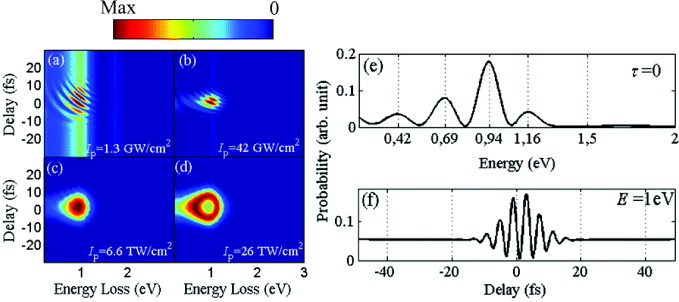
Figure 6. Calculated electron energy-loss spectra versus laser field temporal delay and photon energy. The structure is illuminated with a 2 fs optical pulse at intensities of (a)  , (b)
, (b)  , (c)
, (c)  and (d)
  . The scattered optical pulse is chirped, which is because of multiple plasmonic resonances of the structure. Because of the chirping of the optical pulse the interference fringes become visible in the frequency domain. (e) Probability versus energy at a laser intensity of
  and
and  which shows the beating of 0.25 eV appearing in the energy domain. (f) Probability versus delay at an energy loss of E = 1 eV. The color bar is in arbitrary linear units.
Download figure:
Standard image High-resolution imageThe longitudinal broadening of the electron wave function considered in the previously mentioned investigations was  , which corresponds to a temporal broadening of
  . In order to observe the interference fringes, the longitudinal broadening of the electron wave function should be
  . For the plasmonic resonance at an energy of 1 eV, that would be equal to
  . Figure 7 shows the computed electron energy-loss spectra for the case of an optical pulse duration of 5 fs, a peak intensity of
  , and different longitudinal broadenings for the incident electron pulse. For
  , the interference fringes are well visible, while they start to blur at larger values of W'z and become hardly observable at broadenings larger than
  .
.

Figure 7. Calculated electron energy-loss spectra versus laser field temporal delay and photon energy for a 5 fs optical pulse illuminating the structure at an intensity of  , and the electron pulse with the kinematic energy of 200 keV, and the longitudinal broadenings of (a)
  , (b)
, (b)  , (c)
, (c)  and (d)
  . The color bar is in arbitrary linear units.
Download figure:
Standard image High-resolution imageAlthough attention was mainly paid to the linear electron–photon interaction, nonlinear photon emission and absorption also lead to interference fringes centered at multiples of the incident plasmonic resonant energy of the sample. Figure 8 shows the overall computed electron energy-loss spectra for the case of  ,
,  , and laser peak intensities of
  , 66.4 and
  , depicted in figures 8(a)–(c), respectively. For the computed EELS spectra, the contribution of the nonlinear photon emissions up to n = 3 has been considered. As is obvious from this figure, due to the relatively small broadening of the optical pulse at the resonant energy, the presence of nonlinear electron–photon interactions does not affect the visibility of the interference fringes at the first harmonic.

Figure 8. Calculated electron energy-loss spectra versus laser field temporal delay and photon energy for the longitudinal broadening of the electron wave function equal to  and a 5 fs optical pulse illuminating the structure at a peak intensity of (a)
  , (b)
, (b)  and (c)
  . The color bar is in arbitrary linear units.
Download figure:
Standard image High-resolution image
The reported interference phenomenon depends on the longitudinal broadening of the electron wave function, and of course, as for any other interference phenomenon, the visibility of the interference fringes depends not only on the auto-correlation functions of the electron pulses and the photon pulses, but also on the mutual correlation function of the electron and photon wave functions. Thus the visibility of the interference fringes, if observable in the experiment, can unveil the mutual coherence of the incident photons and electrons.
So far the interaction of electrons and photons has been shown only for the electron trajectory as depicted in figure 2(a). In the supplementary material, the formation of the interference fringes is provided for the other electron trajectories as well. Supplementary figure 1 (available from stacks.iop.org/NJP/15/053013/mmedia) shows the case of the electrons passing from the corner, while supplementary figure 2 (available from stacks.iop.org/NJP/15/053013/mmedia) shows the case of the electrons passing through the center of the nanoprism. For the latter case the electron source cannot interact with the eigenmode at E = 1 eV, so the laser excitation at E = 1 eV is considered as a slightly detuned optical field to interact with the electrons.
4. Conclusion
In this paper, we have demonstrated a systematic investigation of the optical intensities in the context of photon-induced electron energy-loss spectroscopy, by means of a superposition algorithm. While at lower intensities we can explore different modal energies of the nanostructures, by a deliberate tuning of the intensity of the optical beams an interference pattern appears in energy loss spectra in the phase space (energy–time), which is clear evidence of the constructive and destructive interference of the scattered photons from the matter, due to the electron and photon pulses. The reported interference maps in the time–energy space unveil the possibility to acquire the dynamics of the electromagnetic modes, allowing for high spatial, high temporal and high energy resolutions. Moreover, the interference patterns hint at the exploitation of time–energy maps for the phase recovery of the electron wave packet relative to the phase of the optical wave, at huge energy bands in the optical domain.
Acknowledgments
NT gratefully acknowledges the Alexander von Humboldt Foundation for financial support and Professor A Zewail for helpful discussions. The research leading to these results has received funding from the European Union Seventh Framework Programme (FP7/2007-2013) under grant agreement no. 312483 (ESTEEM2).