


Abstract
We propose a method to factor numbers based on the quantum dynamics of two interacting bosonic atoms where the single-particle energy spectrum depends logarithmically on the quantum number. We show that two atoms initially prepared in the ground state are preferentially excited by a time-dependent interaction into a two-particle energy state characterized by the factors. Hence, a measurement of the energy of one of the two atoms yields the factors. The number to be factored is encoded in the frequency of a sinusoidally modulated interaction. We also discuss the influence of off-resonant transitions and the limitation of the number to be factored imposed by experimental conditions.
Export citation and abstract BibTeX RIS

Content from this work may be used under the terms of the Creative Commons Attribution 3.0 licence. Any further distribution of this work must maintain attribution to the author(s) and the title of the work, journal citation and DOI.
1. Introduction
'A series of numbers in arithmetical progression corresponding to others in geometrical progression by means of which arithmetic calculations can be made with much more ease and expedition than otherwise'. At the heart of this quotation from the Encyclopedia Britannica of 1797 [1] is the functional equation

of the logarithm expressed here for two integers p and q. In the present paper, we employ this relation to decompose an integer N = p × q into its factors p and q with the help of two interacting bosonic atoms trapped in a potential with a logarithmic energy spectrum2. Although the scaling of our algorithm does not surpass a classical one, we find that this way of solving a mathematical problem by implementing it in a quantum mechanical system is intriguing.
1.1. The central idea
In the field of cryptography [2], the complexity of prime number decomposition is crucial for the security of codes. However, the Shor algorithm [3] that takes advantage of entanglement of quantum systems has endangered this security reviving an interest in factorization algorithms and creating the thriving field of quantum information [4]. So far, several experiments [5] have implemented the Shor algorithm but in the meantime other approaches such as Gauss sum factorization [6, 7] have been proposed, and realized experimentally.
At first glance our protocol to factor N = p × q is straightforward and simple: we consider two atoms moving in a potential with logarithmic energy spectrum [8]. Starting from the two-particle ground state, we excite them into a two-particle state of total energy E(N) = E0 ln N. A measurement of the single-particle energies might result in E0 ln p or E0 ln q from which we can determine the factors p and q. In this case the problem would be solved.
Unfortunately, in general the situation is much more complicated. Instead of finding the factors p and q one of the following three scenarios may take place: (i) the atoms may still be found in the two-particle ground state. (ii) Due to the identity N = p × q = 1 × N the two-particle state with energy E(N) is at least two-fold degenerate and we could find the integers 1 and N instead of p and q. (iii) Even worse is the possibility that the excitation may bring the atoms into a two-particle state with a different energy E(N') ≠ E(N). This process is quite probable especially when the density of energy levels around E(N) is large. It is needless to say that integer N' may factor in a completely different way.
In this paper we propose a method that guarantees that after the excitation and the subsequent measurement the atoms are found with a probability of nearly unity in the desired states with single-particle energies E0 ln p and E0 ln q. This remarkable feature is a consequence of the fact that only two of all possible two-particle states participate in the quantum dynamics caused by the excitation. The creation of a two-level system consisting of the ground state and the factor state, that is, the state representing the two factors, results from a resonant excitation of the factor state. The other states with this excitation energy have dramatically different transition matrix elements. Indeed, the Rabi oscillations in this two-level system ensure that at half the Rabi period, we end up with the factor state with almost unity probability. Moreover, we can even find an approximate but analytical expression for this time in terms of the parameters of the system. We emphasize that this formula only contains N and is therefore independent of the individual factors. This property allows us to determine the moment at which we have to turn off the excitation and to carry out the energy measurement.
It is interesting to compare and contrast our proposal with the analysis reported in [9], which also addresses the possibilities of factoring contained in logarithmic energy spectra. However, the authors of [9] focus almost exclusively on the limit of a large number of atoms when a description in terms of partition functions is particularly suited. In contrast, we restrict ourselves to two particles. Another major difference between these two approaches lies in the fact that we rely on an explicitly time-dependent interaction, whereas the treatment of [9] by its very nature of using thermodynamical concepts was restricted to a time-independent situation.
1.2. Outline of this paper
This paper is organized as follows. In section 2 we discuss the single-particle states in a potential with a logarithmic energy spectrum and design a time-dependent interaction between two identical bosonic atoms in such a potential which induces a transition preferentially into a two-particle energy state characterized by the factors p and q. Moreover, we introduce in section 3 the two-particle Schrödinger equation governing these transitions.
Section 4 presents our factorization scheme and both, a numerical and an approximate but analytical solution, give insight into the time-dependent probabilities of the two-particle states. Indeed, a numerical example based on typical atomic and trap parameters and neglecting decoherence shows that with our method a correct factorization with more than 90% probability is possible in a single run. However, due to experimental limitations our method is not able to factor arbitrarily large numbers and we carefully discuss these restrictions. A short discussion of the case of more than two prime factors is also addressed. We conclude by summarizing, in section 5, our main results and providing an outlook on possible future developments.
In order to focus on the main ideas while keeping the paper self-contained, we put the details into several appendices. In appendix A we discuss the realization of the one-dimensional (1D) trap and the required effective 1D interaction between the bosonic atoms. In appendix B we show how the dynamics of the two-particle system can be reduced to two levels. Appendix C finally contains an asymptotic treatment of the transition matrix elements needed in our calculations based on the Wentzel–Kramers–Brillouin (WKB) technique [10].
2. One-dimensional model
In this section we briefly introduce our model consisting of three essential ingredients: (i) a logarithmic energy spectrum, (ii) a time-dependent contact interaction between two particles and (iii) bosonic two-particle energy eigenstates. Throughout this section we concentrate on the main ideas; for more details see appendix A.
2.1. Logarithmic energy spectrum
In a recent paper [8], a potential V =V (x) was constructed such that the motion of a non-relativistic particle of mass μ along the x-axis is characterized by a logarithmic energy spectrum

with  . Here we have introduced the frequency

and the energy is not measured with respect to the minimum of V but to the energy E0 = 0 of the ground state.
Given the energy spectrum (1) the time-independent Schrödinger equation

was used to determine iteratively the potential V =V (x) as well as the energy wave functions φℓ = φℓ(x).
In figure 1 we show V together with φℓ for 0 ⩽ ℓ ⩽ 9. In appendix A.1 we describe a method to realize the 1D potential V in a highly elongated cigar-shaped trap.
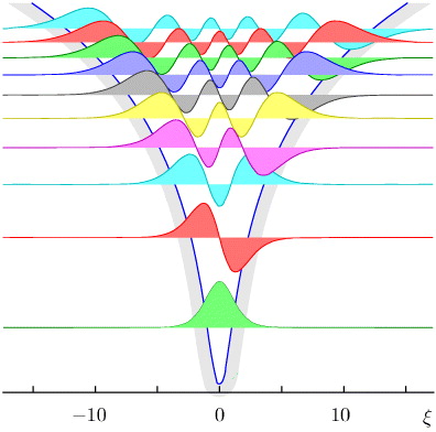
Figure 1. Potential V creating a logarithmic energy spectrum as a function of the dimensionless coordinate ξ ≡ α x with an inverse length α−1 ≡ (μω0/ℏ)1/2 (C.6). This potential was determined numerically [8] by an iteration algorithm based on a perturbation theory using the Hellmann–Feynman theorem and was designed to obtain a strictly logarithmic dependence of the energy eigenvalues Eℓ on the quantum number ℓ. In the neighbourhood of the origin, the potential is approximately harmonic, whereas for large values of ξ it is logarithmic [8]. We also depict the numerically determined energy wave functions of the first ten states in their dependence on the dimensionless position.
Download figure:
Standard image2.2. Quantum statistics and controlled time-dependent interaction
Next we turn to the case of two particles in such a potential. Moreover, for our factorization procedure we need transitions between these two-particle energy eigenstates; that is, we need to introduce a time-dependent interaction between the atoms.
We are considering identical bosonic particles described by the symmetric two-particle energy state


Because these states are stationary for non-interacting particles, we have to introduce an interaction  which we model by a 1D Fermi contact potential [11, 12]

of strength γ, where x1 and x2 are the positions of the atoms. We emphasize that quantum gates based on the time-independent Hamiltonian (6) have been suggested [13] and realized experimentally [14].
In order to induce transitions between the states, we choose a sinusoidal interaction

where the external frequency ωext may be adjusted in such a way as to cause the desired transitions. Moreover, our control over the interaction allows us to switch it on and off.
In appendix A.2 we show that the interaction (7) can be realized experimentally for bosonic atoms in the neighbourhood of a Feshbach resonance [15]. The dependence of the 1D interaction strength γ on both, the s-wave scattering length and the three-dimensional (3D) geometry of the trap, is given in appendix A.3.
The matrix elements of the interaction Hamiltonian given by (6) with the real-valued single-particle eigenfunctions φj read

For bosons, a simple calculation using (4) and (5) gives


where we have assumed r ≠ s and u ≠ v. These matrix elements form the backbone of the quantum dynamics described in the next section.
3. The time-dependent Schrödinger equation for identical particles
The dynamics of the state vector |Ψ(t)〉 of the complete quantum system consisting of two atoms in a 1D potential V and interacting with the time-dependent Hamiltonian (7) follows from the Schrödinger equation

where  is the Hamiltonian of the two non-interacting atoms in V defined by (3).
When we expand the quantum state

into a basis of unperturbed two-particle states |uv〉, we find the coupled equations of motion

for the time-dependent probability amplitudes Ψrs(t). Here we have made use of the expression (7) for the interaction Hamiltonian  with the matrix elements γ κrs,uv given by (8) and

denotes the energy difference between the states |rs〉 and |uv〉.
In the remainder of this paper we shall consider identical bosonic atoms. The matrix elements κrs,uv are understood in the sense of (9)–(11), respectively, but to simplify notation we shall omit the index B henceforth. Equations (13) and (14) remain the same except that the sums now are over indices u = 0,1,2,...,v and v = 0,1,2,... .
4. Factorization
In the present section we apply the model described above and discuss our proposal to factor numbers. After briefly outlining the essential idea we show using the relevant time-dependent Schrödinger equation for the two particles (14) that we can indeed find factors of an integer. Here we pursue two different approaches:
- 1.
- 2.In order to test the quality of the approximations made in approach 1, we keep more equations of (14) and solve the larger system numerically.
We find that the reduction to a two-state system is justified because the corresponding expressions for the occupation probabilities agree rather well.
We conclude by addressing the limitations of our method with regard to the largest integer that can be factored, and by suggesting how to proceed when the number to be factored consists of more than two factors.
4.1. Factorization scheme: a single measurement yields the factors
Suppose that the integer N = pq is a product of two primes p and q and our goal is to find p and q. Our algorithm starts from two non-interacting atoms in the ground state |0,0〉 of our potential with logarithmic energy spectrum (1). At time t = 0 the time-dependent interaction  given by (7) is switched on and the frequency ωext of the harmonic time dependence (7) is chosen to be resonant with the transition into a state of the non-interacting two-particle system with total energy ℏω0 ln N leading to the condition

At some time T we switch off the interaction and a subsequent measurement of the energy of one particle results in ℏω0 ln p'. If the quotient q' = N/p' is an integer not equal to N or 1 we have found both prime factors p = p' and q = q'. We shall show that there exists a time when the probability of finding the two-particle state which contains the factors dominates all the other ones. In addition, we shall give an approximate but analytical expression for this time. We emphasize that in this algorithm we only make a single measurement on a single particle to find both factors.
4.2. Determining the optimal interaction time
In appendix B we show that the complete system of equations (14) can be approximated by the two equations (B.7) which couple the probability amplitudes for the two-particle ground state |0,0〉 and the factor state |p − 1,q − 1〉. In the present section, we derive an approximate but analytic expression for the time T where the probability |Ψp−1,q−1(T)|2 for the two atoms to be in the factor state is large.
We introduce in (B.7) the dimensionless time τ ≡ ω0t as well as the dimensionless matrix element

defined by (8) and arrive at the system

for the approximate probability amplitudes  and
and  For the initial conditions
  and
and  , we immediately obtain the solutions

which describe Rabi oscillations between the ground state and the factor state with the dimensionless frequency

The corresponding probabilities  and
and  for the example of N = 1271 = 31 × 41 discussed in section 4.3.1 are displayed in figure 2 by dashed lines. These curves show that the probability
  reaches unity for the time t = π/(2Ωω0). We study a more realistic example in section 4.3.1 below and find that if we would switch off the interaction at this time the system is found in the factor state with a high probability. Unfortunately, Ω still contains via the matrix element
  the unknown factors p and q. We overcome this dilemma by the relation

following from the definitions (17) and (20) of the dimensionless matrix element  and of Ω, respectively, the expression (C.6) for α and the asymptotic expansion (C.22) of
  . Note again that due to the bosonic nature (10) of our atoms we have multiplied (C.22) by a factor of 21/2 assuming that p ≠ q.
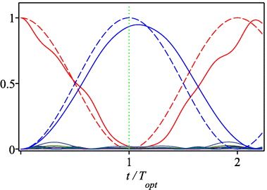
Figure 2. Factorization of N = 1271 = 31 × 41 using two interacting bosonic atoms with parameters given in section 4.3.1 in a potential with a logarithmic energy spectrum. We show the numerically obtained occupation probabilities |Ψ0,0(t)|2 and |Ψ31−1,41−1(t)|2 for the state |0,0〉 (solid red line, starting from unity) and for the state |31 − 1,41 − 1〉 (solid blue line, starting from zero) as a function of time t together with the corresponding expressions (19) based on the secular approximation (dashed lines). The vertical line indicates the approximate optimal time Topt given by (22) to switch off the interaction. Due to the approximations contained in Topt the minimum of |Ψ0,0(τ)|2 is not exactly at that time. Nevertheless, the probability |Ψ31−1,41−1(Topt)|2 of finding the state |31 − 1,41 − 1〉 is as high as 93%. The probabilities for the states resulting from eight off-resonant transitions calculated numerically and shown at the bottom are extremely small and are therefore displayed on a different scale in figure 3.
Download figure:
Standard imageWe emphasize that in the expression (21) the factors p and q do not appear anymore. Hence, we can approximate the optimal time Topt by

where in the last step we have recalled the expression (A.19) for γ.
4.3. Extended model
In the preceding section we have neglected all off-resonant transitions. To test the consequences of this approximation, we include now a finite number M of the off-resonant transitions

nearest to the factor state with p'q' = N ± 1,N ± 2,... in (18). According to (C.19) the matrix elements of the transitions (23) have magnitudes comparable to (B.6) if M ≪ N. We arrive at the (M + 2)-dimensional system
with the dimensionless frequency Δωk ≡ ln N − ln (Pk Qk) and k = 1,...,M.
One might wonder why only in the first of equations (24) additional terms corresponding to off-resonant transitions appear. The explanation for this approximation is as follows. Firstly, we consider 'upward' transitions from the factor state into states with energy ≈ℏω0 ln N2. As shown in appendix C their matrix elements scale with N−1 and therefore we neglect them. Secondly, we consider 'downward' transitions from the factor state into the ground state and states nearby. The nearest state |0,1〉 has an energy of ℏω0 ln 2. Consequently, the term
oscillates much faster than the oscillating terms in the first equation and following the arguments of appendix B is therefore neglected.
The linear system (24) has time-dependent coefficients but with the substitution

it reduces to a linear system with time-independent coefficients which can be solved by a standard numerical procedure.
4.3.1. Example
We consider the case N = 1271 = 31 × 41 and solve (24) subject to the initial condition

for all r + s > 0 taking into account the M = 8 nearest off-resonant transitions. There is no transition into the two-particle state with N' = 1270 because all matrix elements e.g.  vanish by the symmetry of the integrand in (8). But for N' = 1272 four transitions contribute and are taken into account as well as three transitions for N' = 1269 and a single transition for N' = 1273. This results in a system of 20 real equations for 20 unknown real functions since the probability amplitudes are complex.
In section A.3 of the appendix, the interaction strength γ = 2ℏω⊥amax is expressed by the classical frequency ω⊥ of a transverse oscillation in the quasi-1D trap and by the amplitude amax of the oscillating scattering length of the bosonic atoms. As a result the dimensionless matrix element  given by (17) translates into
For our example we consider two  atoms with scattering length a0 = 127 nm [12] in a quasi-1D trap of length 0.2 cm, aspect ratio ω⊥/ω0 = 10, with longitudinal frequency ω0 = 2π × 1000 Hz and the amplitude amax = 1 nm of the oscillating scattering length. These parameters together with the asymptotic expressions (C.19) for the matrix elements κ00,uv derived in appendix C complete the system (24) of equations. Figure 2 shows the time dependence of the occupation |Ψ0,0(t)|2 of the ground state |0,0〉 starting from unity and |Ψ31−1,41−1(t)|2 of the factor state |31 − 1,41 − 1〉 starting from zero due to the initial conditions (25), both in solid lines. A Rabi oscillation between these states is clearly seen. Moreover, figure 2 shows that the probabilities |ΨPk − 1,Qk − 1(t)|2 for the off-resonant transitions are small. They are displayed in figure 3 once more on a different scale.
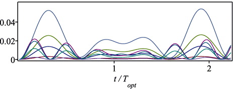
Figure 3. Probabilities for the eight nearest off-resonant transitions calculated numerically from (24) with the parameters given in section 4.4.1 as a function of time t. The probability of finding the off-resonant state |12 − 1,106 − 1〉 (blue line) corresponding to 12 × 106 = 1272 instead of |31 − 1,41 − 1〉 representing the number N = 1271 to be factored is seen to dominate among the others. Nevertheless, it is still severely suppressed.
Download figure:
Standard imageIf we switch off the interaction at Topt indicated by a vertical line in figure 2, the probability that we find the two atoms in the state |31 − 1,41 − 1〉 is 93%, whereas for |0,0〉 it is only 1.7%. The remaining probability is distributed over the states resulting from off-resonant transitions.
We recall that in (B.2) we have derived the condition ωT/N ≫ 2 for the validity of the secular approximation leading to the system (18). Using the parameters of the present example, we find that ω0Topt/N = 9.0, which is larger than two. This is consistent with the result that the transition probabilities calculated from (18) and (24), respectively, and displayed in figure 2 agree reasonably.
The present example is typical in the following sense. The asymptotic condition N ≫ 1 is clearly fulfilled. But the number to be factored is also limited by the experimental conditions as shown in section 4.4. We conclude that the parameters of the example allow us to find the factors of any integer N composed of two prime factors chosen from a range of about 102–104 with a high probability. In section 4.5 we sketch the cases of a different number of prime factors.
4.3.2. Detuned external frequency
Because the energy levels in the logarithmic spectrum (1) become closer and closer spaced as the quantum number ℓ increases, it is obvious that the external frequency must meet the resonance condition ωext = ω0 ln N with a high accuracy. Here we demonstrate that even a small detuning of the external frequency changes the probability of finding the factor state at t = Topt drastically.
We return to our example of section 4.3.1. At N = 1271 we find a spacing ΔΩ = ω0Δω = 5.94 s−1 between the levels N and N + 1. This has to be contrasted with the resonant frequency ωext = ω0 ln N = 4.5 × 10⁴ s−1.
In figure 4 the probability of finding the factor state at time t = Topt is shown as a function of the detuning δω of the external frequency ωext = ω0 ln N + δω as calculated from the system (24). It can be seen that a precision of significantly less than 1 s−1 of the external frequency ωext is required if a single run of the experiment results in the factors with a probability of more than 90%.

Figure 4. Probability P31,41 ≡ |Ψ31−1,41−1(Topt)|2 of finding the factor state |31 − 1, 41 − 1〉 at t = Topt as a function of the detuning δω defined by the relation ωext = ω0 ln N + δω. The other parameters are the same as in figure 2.
Download figure:
Standard image4.4. Estimate of the largest number N to be factored
We now analyse the restrictions on the largest integer N that can be factored by our method which are imposed by the experimental limitations and the model. The most severe condition is dictated by decoherence.
4.4.1. Trap parameters
We begin by considering the properties of the trap and identify two parameters which limit the number N to be factored by the protocol described in this paper. The first one is the aspect ratio ω⊥/ω0 which due to assumption (A.4) to have a 1D trap takes the form

Since this condition involves an exponential it is not the limiting factor.
The length L of a trap is limited by technical reasons and represents the second parameter constraining the number N. According to appendix C we estimate the distance LN between the two classical turning points xN of a particle with energy EN by

which yields with the expression (C.6) for α the inequality

which is an upper bound on N. This condition is more serious than (26) since it scales only linearly.
4.4.2. Off-resonant transitions
The third parameter limiting N is the strength γ of the Fermi contact interaction (6). Indeed, the frequency ωext is chosen to be resonant with the transition |0,0〉 → |p − 1,q − 1〉 where pq = N. We now ask under what conditions transitions into neighbouring states |P − 1,Q − 1〉 with PQ = N ± 1,N ± 2,... have small probabilities.
Consider, for example, the transition |0,0〉 → |P − 1,Q − 1〉 with PQ = N' ≡ N − 1 driven by a frequency ωext = ω0 ln N, which is off-resonant by a detuning
Since Δω decays inversely with N we recognize that with increasing N neglecting off-resonant transitions becomes more and more a problem. If the transition into |P − 1,Q − 1〉 with PQ = N − 1 were the only one possible for the system, we can apply the theory of Rabi oscillations presented in many textbooks [10]. According to this theory, the amplitude of the Rabi oscillation of the transition probability approaches zero as the ratio ℏΔω/|Wif| of the energy ℏΔω corresponding to the detuning and the transition matrix element Wif of the perturbation causing the transition approaches infinity, that is,

Of course, there are many more transitions of our two-particle system but the frequency of the off-resonant transition discussed above is the one closest to the frequency ωext of the perturbation. We now give a rough estimate of how the number N to be factored is limited by the parameters of the trap as well as the interaction strength γ. With the help of the expression (A.16) for γ and the WKB formula (C.22) for the matrix element  , we obtain the inequality

We note that the parameters chosen for the example of section 4.3.1 fulfil the conditions (26)–(28).
4.4.3. Decoherence
Up to now we have not addressed the issue of decoherence. Indeed, it is completely neglected in the system of equations (24). Therefore, decoherence must be negligible at least for the duration Topt of the interaction.
With the help of (22) we cast (29) into the form
which shows that the number to be factored is limited not only by the trap geometry but, most crucially, by the time Tdec the system can be maintained free of decoherence. In our example in section 4.3.1 we find that Topt = 1.83 s.
Energy levels within neutral atoms in optical lattices are reported [17] to have long decoherence times typically in the range of seconds. Instead, in our model the controlled interaction (7) causes transitions between vibrational states of the atoms in the trap. A theoretical work [18] very similar to ours on vibrating neutral atoms in 1D optical microtraps estimates times up to 1 s, which hopefully may improve as technology develops.
4.5. The number of factors different from two
Finally, we briefly discuss three cases where the number of prime factors is different from two. To perform at least an order of magnitude evaluation of the probabilities of finding the prime factors, we assume all of the factors to be of approximately the same size.
We start with the case of three different prime factors N = pqr. Here we must apply the scheme of section 4.1 repeatedly as we now demonstrate. Acting as before with an external frequency ω0 ln N onto the two-particle ground state, it is highly probable that one of the excited states |p − 1,qr − 1〉, |q − 1,pr − 1〉 or |r − 1,pq − 1〉 gets populated, each with a probability of roughly 1/3. Any single-particle energy measurement can lead to one of the six integers contained in these states and if an energy ℏω0 ln ℓ1 is measured, then the integers ℓ1 and ℓ2 = N/ℓ1 are calculated. To find all three factors p, q, r a second run is needed. If here any of the four remaining integers results all three factors can be determined. But if one of the two integers ℓ1 or ℓ2 already known reappears, which happens with a probability of about 1/3, then we ran in the same two-particle state as before and a third run is needed and so on. We estimate the probability of full success with n repeated runs to be of the order 1 − 1/3n−1.
Secondly, consider the case of only one factor, i.e. N is prime, but assume that this is not known to us and we try to apply the protocol of section 4.1 assuming erroneously N would be a factor of two primes. But provided that N is odd only a transition into the state |00,0 N − 1〉 is possible. As discussed in appendix C the Rabi frequency κ00,0 N−1 given by (C.24) is about a factor of N−1/2 smaller than that calculated from (C.22). At the time t = Topt given by (22) the system would with high probability still be in the ground state, and from a measurement resulting in the single-particle ground state it can be concluded that N is prime.
Our last example demonstrates that even with a moderate number of prime factors our protocol becomes impractical because it needs a number of repeated runs. Consider the factorization of N = 1275 = 3 × 52 × 17. From these prime factors five different pairs of integers can be formed whose product equals N = 1275, such as e.g. 15 and 85. We leave it to the reader to convince himself that at least five runs are needed to find the four prime factors and the probability of geting all of them with just five runs has an order of magnitude of about 4%. This means that typically many more runs are needed to find the prime factors.
5. Summary
The logarithm of the product of two numbers is the sum of their logarithms. In the present paper we use this well-known functional relation to propose a new algorithm for finding the two factors of an integer.
Our approach relies on three crucial ingredients: (i) a potential that gives rise to a logarithmic energy spectrum, (ii) two identical bosonic atoms in this potential which interact with each other due to a sinusoidally time-dependent s-wave scattering amplitude whose frequency is proportional to the logarithm of the number to be factored and (iii) a measurement of the final energy of one of the two atoms which provides us with one of the factors.
A remarkable property of this system is the fact that the excitation of the atoms from the two-particle ground state by the time-dependent s-wave scattering populates preferentially a two-particle state whose energy is the sum of the single-particle energies corresponding to the factors. Indeed, we have shown that the full system of equations for the transition probability amplitudes reduces to one consisting of only two levels defined by the two-particle ground state and the state involving the factors.
Rabi oscillations between these two states develop and there is an optimal time at which almost all population is in the state representing the factors. Moreover, with the help of the familiar WKB method we have been able to derive an analytic expression for this time which scales with (N ln N)1/2. Since the logarithm is slowly varying with N our system is analogous to a classical device which by trial and error would also find the factors after  trials.
Our proposal can be implemented with today's cold atom technologies but at the moment does not scale better than a classical device. Several ideas to overcome this barrier offer themselves. Here we only briefly allude to three.
It is the scaling of the time at which we switch off the interaction with N which determines the usefulness of our scheme. Since this time is governed by the Rabi frequency an enhancement factor of this frequency would help. We recall that a single symmetric excitation in an ensemble of cold atoms leads to an enhancement of the matrix elements determined by the square root of the number of atoms involved. Hence, the use of an ensemble of entangled atoms [19] rather than two atoms may well offer an improvement.
Degenerate energy eigenstates of a quantum system are sensitive to perturbations [20] and thereby represent excellent probes of interactions. One prominent example [21] illustrating this statement is the energy levels of the hydrogen atom which feel those vacuum fluctuations of the electromagnetic field giving rise to the Lamb shift. Moreover, the improvement of the Grover algorithm [22] over conventional search algorithms can be traced back [23] to the lifting of degeneracy due to perturbations. Therefore, it is suggestive to employ the large degeneracy of the energy eigenvalues of a large ensemble of atoms in a potential with a logarithmic energy spectrum and lift it by a time-independent interaction. However, in this case we have to deal with distinguishable particles.
The famous Shor algorithm [3] profits from the exponential scaling of the Hilbert space defined by an ensemble of two-level atoms with the number of atoms. Since the underlying principle of our scheme is the two-level dynamics, an improvement may be achieved by using many entangled two-particle systems with a logarithmic energy spectrum.
Needless to say, these three examples are only 'ideas for an idea' and a more detailed analysis is needed before a final conclusion can be drawn. Nevertheless, we find it intriguing that the well-known functional equation of the logarithm can be implemented in a quantum optical realization to solve a fundamental problem in number theory.
Acknowledgments
We thank M Freyberger, H Kübler, T Pfau and G Tanner for many fruitful discussions. RM gratefully acknowledges support from the Graduate School of Mathematical Analysis of Evolution, Information and Complexity at Ulm University.
Appendix A.: Realization of the model
In this appendix we provide an additional background for our factorization scheme. In particular, we show that it can be implemented experimentally. For this purpose we first discuss a possible realization of the 1D potential V giving rise to a logarithmic energy spectrum by a cigar-shaped trap. We then provide a method for constructing the time-dependent interaction using an oscillatory magnetic induction near a Feshbach resonance. Finally, we reduce the 3D scattering length to the one appropriate for our 1D potential.
A.1. A cigar-shaped trap
We consider a rotationally symmetric potential

which is harmonic in the y–z-direction, while in the x-direction the potential V =V (x) gives rise to the logarithmic spectrum (1).
We realize V3D by an optical potential formed by a holographic mask which can create a desired intensity distribution I = I(r) of an electromagnetic field in position space [24]. If the frequency of this radiation is far-detuned from any transition frequency of the atom, the resulting potential V3D = V3D(r) is proportional to I(r) [25]. Hence, it is possible with today's technology to tailor the potential and, in particular, create one that gives rise to a logarithmic energy spectrum.
The energy eigenvalues of a particle of mass μ moving in the potential V3D defined by (A.1) read

with the eigenfunctions

with ℓ,m,n = 0,1,2,.... Here um = um(y) denote the well-known energy wave functions of a harmonic oscillator with mass μ and eigenfrequency ω⊥, and φℓ(x) are the eigenfunctions of the Hamiltonian  discussed in section 4.3.1.
Our quasi-1D model is defined as usual [11]: the transverse quantum numbers m and n of the particle are confined to those of the ground state, that is, to m = n = 0. As long as the longitudinal energy Eℓ is below the energy ℏω⊥, that is,

no transition to an excited transverse state is possible and the energy of the particle is characterized by the longitudinal quantum number ℓ and the trap can be considered to be longitudinal.
A.2. Designing the time-dependent interaction
To model a short-range interaction in three dimensions, one cannot resort to a delta function because it does not influence the dynamics in a scattering process. For pure s-wave scattering, however, the Schrödinger equation can be solved for a pseudo potential acting on a spherically symmetric wave function ψ(r) as

which mimics a hard-core potential with an interaction constant

proportional to the s-wave scattering length a [26]. Acting with the pseudo potential (A.5) on a function ψreg(r) regular at the origin, it simply follows that

(note that δ(x)f(x) = δ(x)f(0)), i.e. here the pseudo potential (A.5) may be substituted by a contact potential.
In this paper we do not solve a Schrödinger equation for the scattering of the two atoms, but instead in our perturbative approach we only calculate matrix elements of the interaction potential with the unperturbed wave functions which are certainly regular everywhere in space. Therefore we are allowed to use the contact potential

in our further calculations. This contact potential is valid for very long wavelengths of the interacting cold atoms.
If the atoms exhibit a Feshbach resonance [15], it is possible to tune the interaction (A.8) between the atoms via the scattering length

which near the resonance B = B0 depends [12] on a magnetic induction B as shown in figure A.1. The parameters B0 and ΔB are determined by the microscopic structure of the atoms [12] but we treat them here simply as phenomenological parameters.

Figure A.1. Realization of a time-dependent interaction between the two bosonic atoms using a Feshbach resonance and normalized s-wave scattering length a/a0 in its dependence on the dimensionless magnetic induction B/B0 (red solid line). The Feshbach resonance appears at B = B0 and a0 is the scattering length far away from the resonance. At B = B0 − ΔB the scattering length vanishes, i.e. the s-wave interaction disappears. The time dependence of the scattering length (A.11) follows when B oscillates around the zero of a(B) as indicated by the orange line.
Download figure:
Standard imageFor a time-dependent magnetic induction B of the form

with amax ≪ a0 the scattering length,

varies sinusoidally with t.
Hence, we have realized the two-atom interaction (7) by a time-dependent magnetic induction B(t) oscillating with frequency ωext around B = B0 − ΔB where the interaction (7) vanishes.
A.3. Effective one-dimensional interaction
We now calculate by following [27] the matrix elements  of the 3D contact potential (A.8) with the unperturbed wave functions 〈xyz|ℓ00〉 ≡ ψℓ00(r) defined by (A.3) using the ground state wave function

with α2⊥ = μω⊥/ℏ.
From the definition

of  and from the expression (A.3) for ψℓmn, we find the formula

After performing the integration of the ground state wave functions (A.12) over y, we find that

Comparison with the 1D matrix element

gives the expression

where we have used (A.6).
When we recall the relation (A.11) for the time-dependent scattering length, we find that

which defines the effective 1D coupling constant

This relation may also be found in [11, 28], but in a different form and with a different derivation.
So far we have considered distinguishable particles. However, in the bosonic case these matrix elements have to be multiplied by the appropriate factors summarized in (9)–(11).
Appendix B.: Reduction to a two-level system
In this appendix we reduce the system of equations (14) for the probability amplitudes Ψrs(t) to arrive at a two-level dynamics. We start from the initial condition |Ψ(0)〉 = |00〉 for the two-particle state vector |Ψ(t)〉 which translates into the initial conditions Ψ00(0) ≡ 1 and Ψuv(0) ≡ 0 for u + v > 0.
Therefore, we first consider the corresponding equation in (14) for the time rate of change in the amplitude Ψ00(t). Using the expression (15) for the frequency Δrs,uv as well as the resonance condition (16), we find that

Next we recall that the average of the oscillating function eiωt over a time interval T obeys the inequality

and therefore becomes small for large ωT. To neglect rapidly oscillating terms in the system (14) corresponds to making the so-called secular approximation or rotating wave approximation [16].
Now we average the oscillating phase factors in the curly brackets in (B.1) over a time interval T large enough that we can neglect all of them except the two in the first term corresponding to the states with quantum numbers u = p − 1 and v = q − 1 and u = 0, v = N − 1. For them the phase factor is unity. We note that from the second phase factor in the curly brackets, no terms survive because here the argument of the logarithm can never be unity. For this reason (B.1) reduces to

In this approximation the amplitude of the ground state couples exclusively to two states, both with energy ℏω0 ln N.
Next we consider the time rate of change
of the amplitude of the factor state and again average the two phase factors in curly brackets over time. But in contrast to (B.3) now five terms survive. Assuming p ≠ q these are in the first phase factor the states with u = p2 − 1, v = q2 − 1, u = pq2 − 1, v = p − 1, u = qp2 − 1, v = q − 1 and u = v = pq − 1. In the second phase factor it is the state with u = v = 0. In this way, (B.4) takes the form
The last term in (B.5) couples the factor state with energy ℏω0 ln N to the ground state while the first four terms couple the factor state to states that all have energies ℏω0 ln N2.
In order to simplify (B.3) and (B.5) even further, we now use scaling properties of the matrix elements κrs,uv discussed in appendix C. Since according to (C.22) we find that

therefore we take into account κ00,p−1 q−1, while the matrix element κ00,0 N−1 which scales with N−1 is neglected in the limit of large N. The matrix elements for the transitions into the four states with energy ℏω0 ln N2 scale with at least N−1 as shown in (C.25) and are therefore also neglected.
Within this approximations we are now left with only the two equations
which couple the ground state and the factor state.
In our derivation of (B.7) we have neglected all oscillating terms in (B.1). To estimate the time T in (B.2), we note that the oscillating terms in (B.1) are multiplied by individual matrix elements. With the help of the WKB-wave functions (C.14), we have estimated that these matrix elements have the same magnitude or are even smaller than those of the constant factors. Therefore, it is sufficient that the time averaged phase factors (B.2) are significantly smaller than unity.
The crucial terms are those which oscillate most slowly. Clearly, these are the ones with (u + 1)(v + 1) = pq ± 1 where we have ω = ω0ln(pq/(pq ± 1)) ≈ ± ω0N−1 in the exponents of the oscillating terms. If the averaging time T is large enough to satisfy

we can neglect all oscillating terms and (B.1) can be approximated by (B.7).
Appendix C.: WKB analysis of transition matrix elements
We may calculate the matrix elements (8) numerically since we have determined the energy eigenfunctions φℓ = φℓ(x) numerically from an iteration algorithm [8] of the time-independent Schrödinger equation (3). However, in order to gain deeper insight into the dependence of φℓ on the quantum number ℓ and the corresponding turning points ± xℓ of the classical motion with energy Eℓ we now pursue a semi-classical analysis using the WKB approximation [10] which is well suited for large integers ℓ. Moreover, we obtain a Gaussian approximation of the ground state wave function φ0. With the help of these expressions we derive approximate but analytical formulae for the matrix elements that allow us to discuss their scaling properties.
C.1. Simplified wave functions
We start with the well-known WKB approximation [10]

of the ℓth single-particle energy wave function valid inside the oscillatory regime and far away from both classical turning points ± xℓ defined by the condition

When we insert the Rydberg–Klein–Rees potential [29] applied to the logarithmic spectrum calculated in [8] into the classical momentum

we find the Bohr–Sommerfeld–Kramers quantization rule

Having in mind that we need the WKB wave functions (C.1) for large indices ℓ only, we use the approximate asymptotic potential [8]

with

to determine the classical turning points

The classical period

is calculated using the action given by (C.4) as well as the energy spectrum (1).
To obtain the scaling properties of our factorization scheme and to completely avoid numerical evaluations, we observe that in the matrix elements

used in section 4.2 the square of the ground state wave function φ0 appears. Because of its limited range shown in figure C.1 the wave functions φℓ(x) with ℓ = p − 1 and ℓ = q − 1 are needed only for values of x close to the origin.

Figure C.1. Comparison of the exact and approximate wave functions φ0,φ31−1 and φ41−1 of the single-particle states used in the example of section 4.3.1 as a function of the dimensionless position ξ = α x. Solid lines show the numerically obtained wave functions, while dashed lines show the simplified WKB wave functions (C.14), and for the ground state wave function φ0, its approximation (C.15). Hence, within the limited range of φ0 these WKB approximations agree well with the numerically obtained wave functions φℓ. Moreover, it shows that expression (C.15) is an excellent approximation to the ground state wave function.
Download figure:
Standard imageThis fact allows us to apply the approximation

Because the numerical treatment of (3) gave V (0) = −0.488 ℏω0 [8], we substitute

into (C.10) and with the help of the relation

which reduces, with the help of the quantization rule (C.4), to

we arrive at the simplified WKB wave function

We note that the wave functions with odd index ℓ vanish at the origin.
Figure C.1 compares this approximation to the numerically obtained wave functions for parameters arising in our example of section 4.3.1. We emphasize that indeed in the neighbourhood of the origin, the two wave functions are in remarkable agreement.
In order to find an approximate analytical expression for the matrix element (A.16), we fit a normalized Gaussian

to the numerically obtained [8] ground state wave function φ0(x) and find that

Again in figure C.1 we compare the numerically exact expression and the approximation and find that there is excellent agreement.
C.2. Scaling of matrix elements
With the approximations (C.14) and (C.15) the matrix element (C.9) for the transition |00〉 → |p − 1,q − 1〉 takes the form

and becomes a standard integral.
Indeed, with the abbreviation

and for p and q both even, or both odd, we find the expression
which reduces with the help of the relation

to

otherwise it vanishes. Hence, the last line shows that the matrix element depends only on the product

We assume that

and approximate (C.20) by
As a consequence, we arrive at the asymptotic expression

no matter whether p and q are both even or both odd.
For N odd the matrix element for the transition |0,0〉 → |N − 1,0〉 given by

yields after integration the asymptotic behaviour

while for N even it vanishes.
For the matrix element of the transition κp−1,q−1 P−1,Q−1 with PQ = N2 it is sufficient here to give a crude estimate which contains four WKB wave functions. With the help of (C.14) it follows that

Again we note that we are considering distinguishable particles here. In the bosonic case the matrix elements must be multiplied by the appropriate factors given by (9)–(11).
Finally, we use the example 7 × 181 = 1267 to illustrate how much our factorization protocol suffers if the factors p and q deviate considerably from the assumption (C.21). Here the approximation (C.22) gives a Rabi frequency which is 70% larger than the frequency (C.19) calculated from factors 7 and 181. As a consequence, the interaction is switched off at a time Topt given by (22), which is too early and the probability of finding the factor state |7 − 1,181 − 1〉 is only 53%. Three runs are therefore needed to find the factors with a probability of about 90%.
Footnotes
- 2
Although we mainly address the case of numbers N consisting of two factors, we shall also point out generalizations of our algorithm to numbers containing more than two factors.