


Abstract
Interactions of a spiral wave with a pacemaker is studied in a mathematical model of two dimensional excitable medium. Faster pacemakers emitting target waves can abolish spirals by driving them to the border of the medium. Our study shows that a slower pacemaker can modify spiral wave behavior by changing the motion of the spiral core. We analyze the dynamics of the spiral wave near the spiral core and away from the core as a function of size and period of the pacemaker. The pacemaker can cause the spiral wave to drift towards it, and either speed up or slow down the reentrant activity. Furthermore, the drift induced by the pacemaker can result in irregular or quasiperiodic dynamics even at sites away from the pacemaker. These results highlight the influence of pacemakers on complex spiral wave dynamics.
Export citation and abstract BibTeX RIS

Content from this work may be used under the terms of the Creative Commons Attribution 3.0 licence. Any further distribution of this work must maintain attribution to the author(s) and the title of the work, journal citation and DOI.
1. Introduction
Excitable media, such as flame fronts during a forest fire [1], the BZ reaction [2], and the heart [3] have certain features in common. They respond to a suprathreshold stimulus with a characteristic wave-like activity, e.g. a flame front, a chemical wave or an electrical wave. After the wave they cannot be excited again for some time, called the refractory period of the medium. The refractory period acts as the waveback of the excitation wave. Excitation waves propagate in space without any attenuation, but they annihilate each other upon collision. In two dimensional excitable media excitation waves are typically target waves emanating from a pacemaker or spiral waves. In spiral waves, the wavefront and waveback meet at the spiral tip. Winfree observed that the tip of spiral wave is not stationary but rotates around a circle (rigid rotation) or moves in complex flower like trajectories (meander or hyper meander) [4]. When the spiral meanders the activation near the spiral core is quasiperiodic [5–8]. Fluctuations in the spiral period because of this quasiperiodic activation is maximum near the core and diminishes as we move away from the core [9, 10]. Studies have shown that the transition from rigid rotation to meander as excitability of the system is varied is a supercritical Hopf bifurcation [11]. Meandering transition of a spiral wave is also related to the Euclidean symmetry of the spiral wave in a plane [11–13]. Apart from the rigid rotation and the meander, the spiral tip in the vicinity of heterogeneities can also drift from its initial location [3, 14].
Various types of nonexcitable or partially excitable heterogeneities in the medium can affect the dynamics of the spiral wave. For example experiments in cardiac tissue [15] and in cardiac cell cultures [16] have found that spiral waves interacting with a nonexcitable tissue or other obstacles can attach to them and assume a rotating frequency determined by the size of the obstacle. Detailed numerical work later established that such attachment depends on the local kinetics near the spiral tip [17] and size and position of the obstacle with respect to the spiral tip [18, 19]. Theoretical and experimental studies demonstrate that spiral waves trajectories can be strongly affected by partially excitable heterogeneities [20–23]. However, the dynamics can be more complex when, on occasion, the wave enters the heterogeneous region. Such complex dynamics were found in monolayers of cultured cardiac cells when the wave interacted with line defects and partial conduction blocks. Time series recorded from near the core of the spiral wave exhibited period-1, period-2 and period-3 oscillations [24, 25]. In numerical studies of wave dynamics in a medium with an ischemic region of reduced excitability Xu and Guevara [26] observed two kinds of spiral formation when the medium was paced with high frequency waves. In the first kind the spiral tip stayed entirely outside the ischemic zone and in the second kind the tip went around the ischemic zone but then returned to the original position through the heterogeneity.
Pumir et al [27] have designed an ischemic zone in monolayers of neonatal rat ventricular cells to study ectopic beat generation and spiral wave initiation. Similarly, we found a novel scenario in which spiral waves are initiated in cultured monolayers of chicken heart cells by the interaction of two pacemakers. We had engineered a pacemaker in the center of the monolayer and induced extra pacemakers in the periphery by applying potassium channel blockers to the monolayer [28]. The dynamic interaction between target waves from the faster side pacemaker in the medium with the central pacemaker led to wave breaks which subsequently formed spiral waves. The spiral wave thus generated then interacts with the pacemaker.
This observation motivates the current work in which we investigate spiral–pacemaker interactions. The spiral–pacemaker interactions can lead to complex spatiotemporal activation in the medium. The resulting dynamics depend on both on the period and the size of the pacemaker. We present the model equations in section 2, and our results in section 3. Implications of these results are discussed in section 4.
2. Model
We use a modified version of FitzHugh–Nagumo (FHN) equations [28, 29], to simulate excitable media and pacemaker dynamics. The equations are:
where v is the excitation variable and w is the recovery variable. The model equation is modified from the standard FHN equation in order to control the pacemaker period independent of the action potential duration. The multiplication factor in the recovery variable, w, allows us to control the duration of the plateau and the resting state independently by parameters wH and wL respectively.
We use D = 0.2 cm2 s−1,  = 0.6 s, β = 0.7 and γ = 0.5. Neumann (no-flux) boundary condition is used along the edges of the simulation domain. In the homogeneous excitable medium, the pacemaker current IP = 0 and wH = wL = 0.06 s−1. See figure 1 for the single cell action potential and the phase plane of this model. In a two dimensional homogeneous medium with this set of parameter values, the medium can support stably rotating spiral waves with period ≈0.73 s. The pacemaker is defined as a central disc with radius rCP in which IP = 1. We use wH = 0.06 s−1 and wL = wLcp inside the pacemaker. With all other parameter values fixed, the pacemaker period, TCP, can be controlled by varying wLcp according to the relationship,
  where T0 ≈ 0.3908 s and θ ≈ 0.0460 [28]. The hyperbolic dependence on wL occurs since wL controls the rate of depolarization of the action potential. The spiral tip was defined as the site (x*,y*) where v(x*,y*),w(x*,y*) have values close to center of the phase plane (v* = 0,w* = 0) (see figure 1), as demonstrated in Winfree [4]. A two dimensional spline interpolation scheme was used to find the site (x,y) which has the minimum distance to (x*,y*). The interbeat interval (IBI) or the spiral period is the time between successive crossing of v = 0.4 with a positive slope at a given spatial location. In this paper we report IBIs measured from the spiral core (denoted as site i, x = 3.5 mm, y = 5.5 mm) and at a point away from the core (denoted as site ii, x = 5.5 mm, y = 5.5 mm).

Figure 1. Single cell dynamics of equation (1) when wL = 0.10. (a) Traces v and w during an action potential, (b) phase plane trajectory (dashed line). Solid lines are the nullclines of equation (1).
Download figure:
Standard imageThe equations are integrated using forward Euler discretization with Δt = 0.5 μs on a 200 × 200 grid with Δx = 50 μm. The size of the simulation domain in dimensioned units is 10 × 10 mm2. We have crosschecked representative numerical results with simulation using fourth order Runge–Kutta numerical scheme, and further with simulations with Δt = 0.125 μs on a 400 × 400 grid with Δx = 25 μm.
The spiral wave is generated using a broken wave front that was allowed to evolve for 100 s in a medium with wL = 0.06 s−1. This state is then used as an initial condition for later simulations.
3. Results
The rotation period of the spiral and its stability are controlled by the parameter wL (figure 2(a)). Spiral tip trajectories for wL = 0.036, 0.048 and 0.06 s−1, are illustrated in the insets of figure 2(a). The wave solution is unstable when wL ⩽ 0.003 s−1. For wL ⩾ 0.003 s−1 the tip meanders in a flower-like trajectory. As we increase wL the medium becomes more excitable, and the spiral wave rotates faster. The amplitude of tip movement decreases with increasing wL, when the system excitability increases [4, 11]. We use wL = 0.06 in the excitable medium, and thus in the absence of the pacemakers, the tip meanders as shown in the figure 2(a) (see also the supplementary movie 1, available from stacks.iop.org/NJP/15/023028/mmedia). Figure 2(b) shows the IBIs from a point near the spiral tip for wL = 0.06 s−1. The time series is quasiperiodic locally near the tip but it is periodic with a period 0.73 s away from it [9].
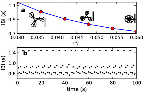
Figure 2. Spiral wave dynamics in the homogeneous excitable medium. (a) Spiral period as a function of wL. Typical tip trajectories for wL 0.036, 0.048 and 0.060 are also shown from left to right. We use wL = 0.06 in the excitable medium. The scale bars along with the tip trajectories are 1 mm. (b) Representative IBIs from the spiral tip (x = 3.5 mm, y = 5.5 mm) when wL = 0.06 (corresponding to the right most tip trajectory in (a)). These IBIs are aperiodic, but IBI from the point away from the tip is 0.73 s.
Download figure:
Standard imageIn subsequent simulations we introduce a pacemaker in the center with wL = wLcp. When wLcp > 0.06 s−1, the pacemaker is faster than the reentrant wave, and it can drive the reentrant spiral out of the medium [30–32]. But when the period of the pacemaker is longer than the period of the reentrant wave, it may still modify the dynamics of the spiral. Let τ denotes the ratio of the spiral period to the period of the pacemaker. We consider 0.012 ⩽ wL ⩽ 0.048 s−1, corresponding to 0.26 ⩽ τ ⩽ 0.75, and 0.2 < rCP < 2 mm.
Initially the spiral tip is located at position (x,y) = (3.5,5.5) mm. When the spiral tip is distant from the pacemaker two possible types of behavior can occur. (i) The spiral waves act to reset the pacemaker leading to the entrainment of the pacemaker, but the spiral tip remains distant from the pacemaker. For example, figure 3(a) shows an example of 1:1 entrainment of the pacemaker by the spiral when τ = 0.26 and rCP = 0.20 mm. (ii) The spiral waves migrate towards the pacemaker and eventually leads to dynamics in which asymptotically the spiral tip is inside or adjacent to the pacemaker boundary for some or all of the time (figure 3(b)). Although these situations are worthy of further investigation, in the current work we focus attention on situations in which the spiral tip has direct interaction with the pacemaker.
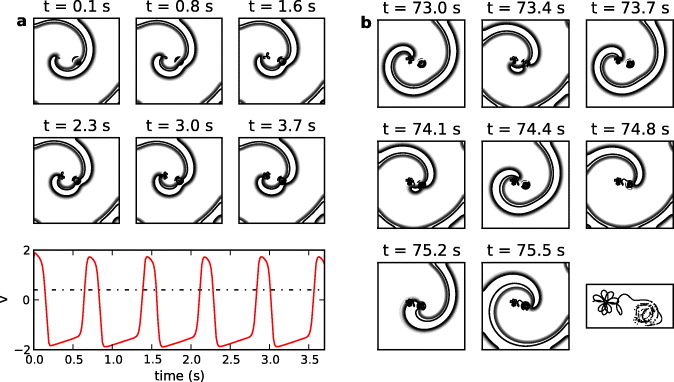
Figure 3. Contour plots of v when a pacemaker with τ = 0.26 and rCP = 0.4 mm is present in the medium. Darker lines indicate higher amplitudes of v. (a) Initially the spiral tip is outside the pacemaker and the spiral arm entrains it. The panels are 0.73 s apart (period of the spiral). The amplitude of action potential measured from the center of the pacemaker is also shown. The dashed line indicates the threshold for measuring the IBI. (b) Subsequently the spiral drifts towards the pacemaker. The panels are 0.36 s apart. Points inside the pacemaker represent positions of spiral tips during a breakup of the wave at that location. The spiral velocity increases when the tip interacts with the pacemaker, as indicated by an increase in the wavelength. The tip trajectory is reproduced in the last panel (see supplementary movie 2, available from stacks.iop.org/NJP/15/023028/mmedia).
Download figure:
Standard imageWe consider three types of direct spiral pacemaker interaction:
Type I. The spiral tip is inside the pacemaker and the dynamics depend on the period of the pacemaker. The spiral either rotates rigidly or meanders so that the trajectory of the spiral core is either circular or has a petal geometry.
Type II. The spiral tip stays on the periphery of the pacemaker or is exterior to the pacemaker.
Type III. The spiral tip executes complex trajectories in which it is partially in the interior of the pacemaker and partially on either the circumference or the exterior of the pacemaker.
Regions of different types of dynamics as a function of τ and rCP are summarized in figure 4(a). This is a schematic representation for which we varied rCP from 0.2 to 2.0 mm and wLcp from 0.012 to 0.048 s−1 in steps of 0.006 s−1 (corresponding to τ values from 0.26, 0.37, 0.47, 0.55, 0.62, 0.69, and 0.75). When rCP = 0.4 mm, for τ < 0.6, we observe type III behavior, i.e., the tip trajectories move inside and outside the pacemaker. This can lead to quasiperiodic or irregular dynamics in the medium. Type II behavior is observed when τ = 0.26, and rCP > 0.4 mm (inwardly rotating petals) or when τ = 0.75, with outwardly rotating petals. For intermediate values of τ and rCP one observes type I dynamics.
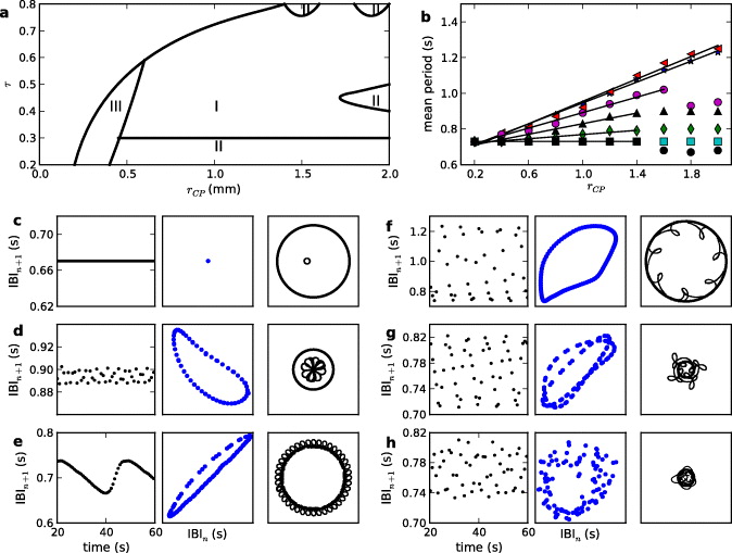
Figure 4. Spiral wave dynamics in presence of the pacemaker. (a) Schematic diagram of spiral tip dynamics in the rCP − τ parameter space. Regions of type I, II and III dynamics are indicated. In the unmarked region the spiral wave is unaffected by the pacemaker. (b) Mean spiral period in the medium as a function of rCP for τ = 0.26 ( ), 0.37 (
 ), 0.47 (
 ), 0.55 (▵), 0.62 (
 ), 0.69 (
 ) and 0.75 (•). The straight lines are best fit lines passing through the linear regime in the data (see text for details). (c)–(h) IBIs, and IBI return plots, and tip trajectories when the spiral tip interacts with the pacemaker. (c) τ = 0.75 and rCP = 1.8 mm, type I dynamics. (d) τ = 0.4 and rCP = 1.0 mm, type I dynamics. (e) τ = 0.75 and rCP = 1.6 mm, type II dynamics. (f) τ = 0.47 and rCP = 2 mm, type II dynamics. (g) τ = 0.47 and rCP = 0.4 mm, type III dynamics. (h) τ = 0.26 and rCP = 0.4 mm, type III dynamics.
Download figure:
Standard imageWhen the spiral tip meanders, the period of the spiral wave measured in the medium depends on the distance of the measuring site from the spiral tip. For example, in the homogeneous medium the time series measured from a site near a meandering tip is quasiperiodic, but it is nearly periodic if measured from a site away from the tip [9]. We take time series from x = 7.5 mm, y = 7.5 mm (site ii), away from the spiral tip and the pacemaker, to represent the global dynamics in the medium. In the homogeneous medium variation in the spiral period at this location is less than 2% of the mean period. The mean spiral period in the medium is also a function of the pacemaker period (τ) and its radius (rCP). Figure 4(b) shows that, for τ = 0.26 and 0.37, the mean spiral period from site ii increases linearly with rCP, similar to what happens during spiral attachment with non-excitable boundary [16]. But for larger τ the spiral period in the medium depends more on τ and less on rCP. For example, in figure 4(b), when τ is 0.47 and 0.55, the mean spiral period increases with rCP but then becomes nearly constant for rCP > 1.4 mm. Then for τ = 0.69 the mean spiral period is independent of rCP, and for τ = 0.75 the spiral is faster than in the homogeneous medium. The best straight line passing through the linear regime is also shown in figure 4(b). The goodness of fit values (R2) for the linear regime is as follows: 0.998 (τ = 0.26), 0.996 (τ = 0.37), 0.991 (τ = 0.47), 0.984 (τ = 0.55), 0.969 (τ = 0.62) and 0 for (τ = 0.69 and 0.75).
However the fluctuation from the mean period in presence of the pacemaker varies as much as 50%, depending on the type of dynamics (see the supplementary figure S1, available from stacks.iop.org/NJP/15/023028/mmedia for standard deviations from the mean in the distribution of IBIs). Variation in the spiral period is more pronounced for type II and type III dynamics, but it is less than 5% for type I dynamics. Examples of spiral tip trajectories and associated IBIs and IBI return plots are given in figures 4(c)–(h). The IBI and its return plots are calculated from a time series measured at a point away from spiral tip and the pacemaker (at site ii). Details of the dynamics in each of these regions are described below.
3.1. Type I: spiral inside the pacemaker
Typical tip trajectories during type I dynamics are shown in figures 4(c) and (d). In figure 4(c) the parameters are τ = 0.75 and rCP = 1.6 mm, and the corresponding tip trajectory is circular. The period of the spiral in the medium is 0.67 s, i.e. the spiral is faster when the pacemaker is present. Parameters in figure 4(d) are τ = 0.4 and rCP = 1.0 mm. The tip meanders in a flower-like trajectory, and the global dynamics is periodic. The amplitude of the meander during the type I dynamics decreases as τ increases, and the spiral period measured at site (7.5,7.5) mm shows less than 2% variation in the IBIs.
3.2. Type II: spiral attachment at high τ, Doppler effect
Type II dynamics (i.e. the spiral attached to the boundary of the pacemaker) are observed in two variants. When τ = 0.75 and rCP = 1.8–2 mm the spiral rotates around the pacemaker with outwardly rotating flower petals (figure 4(e)). The spiral tip moves along the boundary while tracing one petal for every rotation of the spiral in the medium. Because of the movement of the tip around the pacemaker, the tip moves towards the measuring site half the time and away from the measuring site during the other half, causing Doppler shifts in the measured period. As a result the IBIs (figure 4(e); see also the supplementary movie 3, available at stacks.iop.org/NJP/15/023028/mmedia) oscillate between 0.66 and 0.74 s. However, we observe an asymmetric distribution of IBIs in figure 4(e), i.e. there are more incidences of the wave speed up. As the tip moves away from the measuring site, the wave has to travel through the pacemaker with a higher conduction velocity. Hence the IBI decreases even though the tip is moving away from the measuring site.
3.3. Type II: spiral attachment at low τ
When τ = 0.27 we observe another variant of type II dynamics, where the spiral rotates around the pacemaker with inwardly turned petals (figure 4(f)). The pacemaker has a long refractory period in this parameter regime. During the refractory period the spiral cannot enter inside the pacemaker, hence it moves around it. As the pacemaker recovers from the refractory period, the tip enters inside the pacemaker while the spiral arm moves across the pacemaker. The motion of the spiral tip around the pacemaker is similar to the early observation by Krinski on inhomogeneity induced drift [20]. The spiral meander and its drift around the pacemaker lead to quasiperiodic dynamics in the medium. The IBIs measured from (7.5, 7.5) mm (figure 4(f)) are aperiodic, but the IBI return plot has a clear ring structure consistent with quasiperiodic dynamics (see also the supplementary movie 4, available from stacks.iop.org/NJP/15/023028/mmedia for another example).
3.4. Type III: torus doubling and irregular dynamics
In type III dynamics the spiral tip moves partly inside and partly outside the pacemaker. This occurs when the pacemaker size is comparable to the size of the spiral core in the homogeneous medium. Smaller pacemakers (rCP = 0.2 mm) do not have any effect on the spiral wave dynamics. When rCP = 0.4 mm, the wave drifts towards the pacemaker after a long transient (figure 3). However, the pacemaker is not big enough either to enclose the spiral tip within it (type I dynamics) or to allow it to move around the boundary (type II dynamics). As a result the tip meanders as it drifts around the pacemaker, moving partly inside and partly outside the pacemaker. When the wave can enter inside the pacemaker every time (τ = 0.33) the tip trajectory is regular but more complicated than simple type I or type II. The spiral tip meanders in a three-petal flower trajectory that repeats about four times as the tip drifts around the pacemaker (figure 4(g)). The IBIs are still aperiodic, but the IBI return plot (figure 4(g)) shows two rings, as seen during a period doubling bifurcation on a torus [9, 33] (see also the supplementary movie 5, available at stacks.iop.org/NJP/15/023028/mmedia).
But when τ = 0.26, the spiral cannot entrain the pacemaker. During the initial transient dynamics the spiral core remains outside the pacemaker and while spiral arm entrains the pacemaker in 12:10 fashion. After this transient dynamics, the spiral drifts towards the pacemaker (figure 3(b)). The combination of drift and meander inside and outside the pacemaker makes the trajectory irregular. The wave often breaks up several locations inside the pacemaker. The IBIs are aperiodic, varying between 0.74 and 0.82 s (figure 4(h)). The return plot between IBIn and IBIn+1 are partially filled discs. Thus the global dynamics in the medium is irregular even though there is a single spiral wave in the medium.
3.5. Multistability
The effect of spiral wave interactions with unexcitable boundaries decay exponentially as a function of the distance of the spiral tip from the boundary [34]. Similarly the effect of the pacemaker on the wave dynamics depends on the relative position of the spiral tip with respect to the pacemaker. For example, consider the initial condition employed in this study, figure 5(a). With τ = 0.75 and rCP = 1.8 mm, the final dynamics for this initial condition is type II. However, if the spiral tip was closer to the pacemaker the tip can enter inside the pacemaker, resulting in type I dynamics. On the other hand, if the initial location of the spiral tip was farther, the spiral wave is unaffected by the pacemaker.
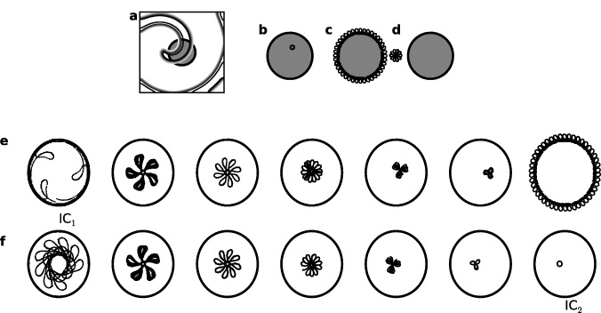
Figure 5. (a) Contour plots of v at time t = 0. The location of a pacemaker with rCP = 1.6 mm and τ = 0.75 placed at the center (5.00 mm, 5.00 mm) is shaded in gray. (b) Spiral tip moves inside the pacemaker when the pacemaker is at (4.75 mm, 5.00 mm). (c) Spiral tip trajectory when pacemaker is at (5.00 mm, 5.00 mm), and (d) when pacemaker is at (5.00 mm, 5.25 mm). (e) Final tip trajectories starting with a spiral initial condition as in IC1 (first panel) for τ = 0.37, 0.47, 0.55, 0.62, 0.69 and 0.75 (from the second to the last panel). (f) The trajectories starting with a spiral initial condition as in IC2 (last panel) for τ = 0.26, 0.37, 0.47, 0.55, 0.62 and 0.69 (first five panels).
Download figure:
Standard imageTo illustrate the initial condition dependence on the spiral pacemaker interaction, we show dynamics starting from two different initial conditions. Consider a pacemaker with τ = 0.27 and rCP = 1.8 mm located at (1,1) mm. The initial position of the spiral as in figure 5(a) is the initial condition used throughout this study. Let this initial condition be IC0. Starting from IC0 with the specified pacemaker will lead to type II dynamics, and the final tip trajectory is as shown in the first panel of figure 5(e). Call this state IC1. Using the spiral position as in IC1 as the initial condition, we vary τ and let the dynamics continue for 10 s. The resulting tip trajectories for τ = 0.37, 0.46, 0.55, 0.62, 0.69 and 0.75 are shown in figure 5(e). Similarly, starting from IC0 with the pacemaker of same size (rCP = 1.8 mm) but with τ = 0.75, the final dynamics is type I, with a tip trajectory as shown in the last panel of figure 5(f). Let this be IC2. The tip trajectories obtained by using IC2 as the initial condition for pacemakers with τ varying from, 0.27 to 0.69 are shown in the first six panels of figure 5(f). In this example the final tip trajectories are independent of the given initial conditions (i.e. IC0, IC1 and IC2) for intermediate values of τ (0.26 < τ < 0.75). But for τ = 0.27, the final dynamics is type II if started from IC0, and type I if started from IC2. Similarly, for τ = 0.75, the final dynamics is type I if started from IC0, and type II if started from IC1.
4. Discussion
Our study shows that local heterogeneities like pacemakers can change spiral wave dynamics in an excitable medium and can lead to quasiperiodic or irregular dynamics. In particular, when the pacemaker is slower than the spiral wave three different types of dynamics can occur, depending on the radius and period of the pacemaker. The spiral wave can move inside the pacemaker (type I), can drift and meander along the boundary of the pacemaker (type II), or it can move partly inside and partly outside the pacemaker (type III). Type I dynamics can lead to periodic or quasiperiodic activation, depending on the period of the pacemaker. In type II dynamics, activation in the medium is quasiperiodic while in type III, the dynamics can also be irregular. The types of dynamics as a function of period and the radius of the pacemaker are summarized in the schematic diagram (figure 4(a)).
There have been a large number of earlier studies concerned with the interaction of spiral waves with heterogeneities. It is well known that spiral waves can become anchored to localized heterogeneities [15, 16, 18, 19], and that global gradients of excitability in the medium can lead to the drifting of spiral waves [35]. The work most closely related to ours involves the study of the effect of localized partially excitable heterogeneities on spiral wave dynamics. As in the current work, localized heterogeneities can lead to the drift of spiral tips. Asymptotically, the spiral tip can be entirely internal to the heterogeneity or remain on the periphery [20, 22–25], similar to what we have observed in figure 4.
In addition to these behaviors, in the current work we have found that the spiral tip can display complex dynamics that can be partially characterized by considering the return map showing the dependence of the IBI in the excitable medium on the preceding IBI (figure 4). Unlike the situation during quasiperiodic dynamics when the return map is a closed curve, we have found two variants. For R = 0.47 rCP = 0.4 mm, figure 4(g), there appears to be a structure similar to those observed in period doubling bifurcations on a torus [33] and also during spiral wave activity in the Luo–Rudy model of cardiac wave propagation [9]. When R = 0.26 rCP = 0.4 mm, the dynamics are more irregular and the IBI return map appears random (figure 4(h)). Although this is qualitatively similar to what was observed during spiral breakup [9], in the current situation the spiral wave does not break up.
These observations may be relevant to clinically observed cardiac arrhythmias. The cardiac rhythm is normally set by a localized pacemaker called the sinus node located in the right atrium. In sinus node reentrant tachycardia there is a reentrant wave centered in the vicinity of the sinus node. It is a relatively rare arrhythmia and is difficult to characterize [36, 37]. Further work is needed to clarify if rhythms similar to those described here are observed in sinus node reentrant tachycardia or other reentrant tachycardias that appear to circulate on a micro rather than a macro reentrant pathway.
Independent of the clinical utility, the current paper highlights a range of complex dynamics that are expected in excitable media with embedded localized pacemakers. The mathematical model used simplifies underlying structural and biophysical details of cardiac pacemakers. It will be interesting to compare our results with those from models which incorporate anatomical details and ionic mechanisms. This would help identify both basic and detailed ingredients important for spiral wave generation, maintenance and termination. It will also be of interest to better characterize the boundaries for the different dynamical regimes and to compute the bifurcations that arise as the size and period of the pacemaker are varied.
Acknowledgments
We thank NSERC and the Centre for Applied Mathematics in Bioscience and Medicine (McGill University) for financial support.