


Abstract
It is shown that a laser wakefield driven in the highly nonlinear regime or the wave-breaking regime in underdense plasma can emit ultra-broad-band bright extreme ultraviolet (XUV) radiation pulses, which are as short as a few hundreds of attoseconds in one-dimensional simulations and a few femtoseconds in multi-dimensional cases. The emission is caused by a transverse current sheet co-moving with the laser pulse. This current sheet is formed by an electron density spike with trapped electrons in the wakefield with a certain transverse kinetic momentum of electrons left behind the laser pulse. This residual momentum appears when the laser pulse undergoes a strong self-modulation and subsequent pulse steepening at the front. In the multi-dimensional simulations, the XUV emission is found only near the laser axis with a much smaller spot size than the laser pulse due to its transverse ponderomotive force effects. The present scheme provides an alternative method for producing single bright ultrashort XUV pulses for ultrafast applications.
Export citation and abstract BibTeX RIS

Content from this work may be used under the terms of the Creative Commons Attribution-NonCommercial-ShareAlike 3.0 licence. Any further distribution of this work must maintain attribution to the author(s) and the title of the work, journal citation and DOI.
1. Introduction
The advent of bright ultrafast x-ray pulses from free electron lasers [1] such as the Linac Coherent Light Source (LCLS) has made possible the time-resolved study of electronic dynamics of various matter states and the exploration of nonlinear physics at ultrashort wavelengths [2]. Meanwhile, to satisfy the huge demand for such sources, a great deal of effort has been made to generate bright x-rays with unique features on a table-top scale by the use of ultrashort intense laser pulses. Various schemes have been proposed, such as high-order harmonic generation derived from the nonlinear interaction of an infrared femtosecond field with a gaseous [3–6] or solid target [7–11], betatron radiation from laser wakefield accelerated electrons [12–15], nonlinear Thomson scattering [16–18] and so on. So far, it is still very challenging in experiments to produce coherent x-ray emission with both ultrashort duration and high intensity.
In this paper, we propose a novel scheme for ultrashort intense extreme ultraviolet (XUV) pulse generation, which is quite different from the methods mentioned above. It is completely based on highly nonlinear wakefields in underdense plasma driven by an ultrashort intense pulse currently available. Such laser wakefields have been widely used in electron acceleration [19–20], laser pulse frequency up-shift (or photon acceleration) [21–22], laser pulse compression [23–25], terahertz radiation generation [26], as well as a flying mirror for x-ray generation [27–28]. Here, we found that when the laser pulse undergoes a strong self-modulation and self-steepening at the front [29–30], the carrier phase of the laser pulse changes dramatically with time. As a result, the electrons can obtain net acceleration transversely in the laser polarization direction as the laser pulse passes by. When the electron transverse velocity beats a high density spike composed of trapped electrons in the wakefield behind the laser pulse, a highly localized current density is produced, which moves at nearly the speed of light and emits ultrafast broad-band intense XUV pulses. This was demonstrated by particle-in-cell (PIC) simulations.
2. One-dimensional (1D) particle-in-cell (PIC) simulations
2.1. 1D simulation of attosecond pulse emission
First, let us start by presenting the results on XUV attosecond emission from one-dimensional (1D) PIC simulations with the code KLAP-1D [31–32]. In the PIC simulations, we take a laser pulse with an amplitude profile a = aL sin2 (π t/τ ) , where aL = 10 is the normalized peak amplitude corresponding to a laser intensity of 1.37 × 10²⁰ W cm- 2 at a laser wavelength of λL = 1 μ m , and τ = 10TL is the full laser period with TL being the oscillating period of the incident laser. We assume that the laser pulse is linearly polarized along the z-direction and propagates along the x-direction in uniform plasma with a density of ne /nc = 0.04 , where nc is the critical density. The left plasma boundary is located at x = 20λL and the plasma length is 200λL . We chose the cell size of λL /200 to ensure enough resolutions in time and space under which we can observe the attosecond pulse emission properly. This is due to the fact plasma wave-breaking is a highly nonlinear process and the trapped electron bunch structure is sensitive to the space and time resolution in the simulation.
Figure 1 illustrates the evolution of the laser pulse and its wakefield (shown by the electron density), as well as the subsequent attosecond pulse generation. In figure 1(a), a high electron density spike is shown behind the laser pulse, which is due to the excitation of the high-amplitude laser wakefield by the ponderomotive force and subsequent electron trapping. At a later time t = 100TL , the laser pulse front steepens, which also drives a density peak at the pulse front, as shown in figure 1(b). At t = 150TL , the laser pulse shortens significantly and the density peak at the front of the laser pulse is still there. But the density spike behind the laser pulse disappears, as shown in figure 1(c). During the laser pulse evolution, one may note that an extremely short pulse emerges near the density spike behind the driving laser pulse. Figures 1(d)–(f) display zoomed-in plots of the extremely short pulses from figures 1(a)–(c). One may note that its amplitude seems to increase with time and its duration also increases from sub-cycle to about one and a half cycles from t = 50TL to 150TL . At the latter time, the pulse has a duration of about one-seventh of the incident laser period or about 460 attoseconds.
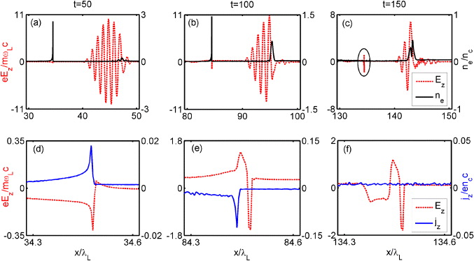
Figure 1. Snapshots of the laser field (normalized by mωLc/e, red dashed lines) and the electron density (normalized by nc , black solid lines) are plotted in (a)–(c) at time t = 50TL , 100TL and 150TL . Encircled in panel (c) is an XUV attosecond pulse propagating behind the laser pulse. Snapshots of the transverse current densities (blue solid lines) and the resulting attosecond pulses (red dashed lines) near the electron density spike behind the driving laser pulse are plotted in (d)–(f) at time t = 50TL , 100TL and 150TL .
Download figure:
Standard image2.2. Additional simulation results with different parameters
In figure 2, we plot the attosecond pulse in vacuum after passing through the plasma region of about 200λL and its frequency spectrum (shown by black solid lines) under the same laser and plasma conditions as in figure 1. Even though the whole duration of the attosecond pulse is about TL /7 , its frequency spectrum extends to over 70ωL . This implies that one may get attosecond pulses with the duration around TL /70 when the low-frequency components are filtered out. Note that the normalized peak field is close to 2.0, corresponding to an intensity over 4 × 10¹⁸ W cm- 2 .

Figure 2. The electric fields of the XUV attosecond pulses detected at the right boundary (a) and the corresponding frequency spectra (b) under different laser pulse duration and plasma electron densities, where the normalized peak amplitude was aL = 10 and n = ne /nc .
Download figure:
Standard imageWe have conducted a series of simulations by changing the plasma density, the laser duration and the laser intensity. It is found that the attosecond pulse generation is a robust process as long as highly nonlinear wakefields are excited and the driving laser is self-modulated and steepened significantly. Therefore, it usually requires a laser intensity in excess of 1019 W cm- 2 , while ours is 4.2 × 10¹⁹ W cm- 2 for aL = 10 and n = 0.04 . In this case, the produced laser wakefields just break after the first wave bucket and the attosecond pulse emerges in the first wave bucket. In figure 2, the attosecond pulses produced with different pulse durations at different plasma densities are shown together with their spectra. It shows that as long as the attosecond pulses are produced, their peak amplitudes do not change significantly with the laser and plasma parameters and their durations are typically around a few hundreds of attoseconds. The pulses have ultrabroad spectra in the XUV range with the spectrum widths, decreasing slightly with increasing plasma densities. One also expects that the duration of the attosecond pulses depends upon the pump laser intensity and plasma density. For example, for the laser parameters aL = 10 and τ = 10TL and the plasma density ne /nc = 0.04 , one observes the attosecond pulse roughly with 3/2 cycles as shown in figure 2. However, one observes an attosecond pulse with nearly five cycles when taking aL = 40 , apparently due to the fact that the driving laser can propagate a longer distance before it is depleted.
3. Theoretical model
3.1. The formation of residual electron momentum
Since the attosecond pulse observed in the simulation is coherent emission, it is related with a transverse electron current. Simulation indicates that it is produced by the current produced near the density spikes of the wakefield behind the laser pulse. In figures 1(d)–(f), we plot snapshots of the transverse current distributions, which are located near the attosecond pulse. Actually, they co-move with the electron density spike. Firstly, according to the continuity equation of the electron fluid, the electron density can be described as n = n0 /(1 -v/vg ) , where vg is the group velocity of the laser radiation in the ambient plasma. A density spike appears around the positions where electrons move with a velocity close to vg . If one assumes that the electron density spike can be described by nspike = δ (x - vg t) , then the transverse current can be written as

where vz is the slowly varying transverse electron velocity near the density spike along the laser polarization direction to be discussed later. As shown in figure 1(c), the electron density spike disappears at t = 150TL , because the driving laser pulse has been depleted significantly and the laser wakefield decreases. Then the transverse current disappears correspondingly as shown in figure 1(f). Afterwards, the attosecond pulse is found to propagate in underdense plasma without visible changes for a long distance. It is thus clear that the transverse currents related with the electron density spikes are responsible for the attosecond pulse generation. In the following, we shall show how the transverse electron velocity vz is produced in the z-direction or the laser polarization direction.
Figure 3(a) displays snapshots of longitudinal distributions of the laser field and the transverse kinetic momentum of electrons pz in the laser polarization direction. Before t = 50TL , one observes that pz has not vanished only inside the laser pulse, which are basically described by  following the canonical momentum conservation, where az is the normalized vector potential. Behind the laser pulse, one finds that pz = az ≈ 0 . At later times, one finds that pz and az do not vanish behind the laser pulse. Instead, they take a single finite value at a given longitudinal position and are distributed in a wide space behind the laser pulse. In the following, we call the finite kinetic momentum of electrons behind the laser pulse as the residual momentum. Note that the change in the residual momentum with the space coordinate is much slower than that found inside the laser pulse; the latter changes in a period of the laser wavelength. The occurrence of this residual momentum is related with the violent evolution of the laser pulse front with time, which includes the changes in the carrier phase of the laser pulse and the pulse front steepening. These are caused by two well-known nonlinear effects, namely the relativistic nonlinearity and the ponderomotive force of the laser pulse. According to the refractive index of a homogeneous plasma, η = (1 - γ- 1
ωp2 /ωL2 )1/2 where γ is the relativistic factor and ωp = (4π n0
e2 /me )1/2 is the electron plasma frequency; the relativistic nonlinearity changes the refractive index in such a way that the high-intensity part of the laser can propagate at a high speed. The ponderomotive force at the pulse front drives a density peak, which induces a frequency down-shift of the pulse front [15]. Both effects tend to produce pulse front steepening and carrier phase changes. At t = 150TL , the laser pulse is depleted to nearly a single cycle, and the residual momentum becomes negative behind the pulse.
following the canonical momentum conservation, where az is the normalized vector potential. Behind the laser pulse, one finds that pz = az ≈ 0 . At later times, one finds that pz and az do not vanish behind the laser pulse. Instead, they take a single finite value at a given longitudinal position and are distributed in a wide space behind the laser pulse. In the following, we call the finite kinetic momentum of electrons behind the laser pulse as the residual momentum. Note that the change in the residual momentum with the space coordinate is much slower than that found inside the laser pulse; the latter changes in a period of the laser wavelength. The occurrence of this residual momentum is related with the violent evolution of the laser pulse front with time, which includes the changes in the carrier phase of the laser pulse and the pulse front steepening. These are caused by two well-known nonlinear effects, namely the relativistic nonlinearity and the ponderomotive force of the laser pulse. According to the refractive index of a homogeneous plasma, η = (1 - γ- 1
ωp2 /ωL2 )1/2 where γ is the relativistic factor and ωp = (4π n0
e2 /me )1/2 is the electron plasma frequency; the relativistic nonlinearity changes the refractive index in such a way that the high-intensity part of the laser can propagate at a high speed. The ponderomotive force at the pulse front drives a density peak, which induces a frequency down-shift of the pulse front [15]. Both effects tend to produce pulse front steepening and carrier phase changes. At t = 150TL , the laser pulse is depleted to nearly a single cycle, and the residual momentum becomes negative behind the pulse.
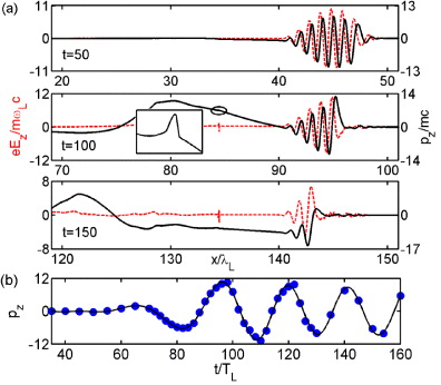
Figure 3. (a) Snapshots of the longitudinal distributions of the laser field Ez (red dashed lines) and the transverse kinetic electron momentum p (black solid lines) at three different time steps. Inset: zoomed-in plot of pz near the attosecond pulse at t = 100TL . (b) Temporal evolution of the transverse electron momentum for electrons located near the density spike behind the laser pulse. The dots are from the simulation and the solid line is a fitted curve. The laser and plasma parameters are the same as those in figure 1.
Download figure:
Standard imageFigure 3(b) illustrates the evolution of the residual electron momentum at a distance about 6λL behind the laser pulse. It shows that the residual momentum begins to build up after t = 50TL due to strong pulse evolution. They even change with time periodically and the time scale for this periodic change is roughly given by 2π ωL /ωp2 , which is the typical time scale of self-modulation. It is clear that the slowly varying residual transverse momentum and the electron density spikes behind the laser pulses are responsible for the formation of the fast-moving narrow current sheet, which emits attosecond pulses.
3.2. A simple model for the attosecond pulse formation
In the following, we give a simple estimation of the attosecond pulse amplitude in terms of the electron current. For the moment, one can neglect the oscillation of the transverse velocity vz because it varies slowly as compared to the density spike. Then according to equation (1), the transverse current can be considered as a function of τ = t-x/vg only. Substituting it into the wave equation

the emitted pulse is given by

where rg = (1 - vg2 /c2 )- 1/2. Further assuming that the density spike is described by δ = nmax sin [(ωatto (t -x/vg )] with 0 ⩽ ωatto (t -x/vg ) ⩽ π , where nmax is the peak of the density perturbation, ωatto is the frequency of the attosecond pulse, whose estimation will be given in the following, and vg /ωatto is the full-width of the density spike, the current is given by

with j0 = evz nmax . From equation (2), it gives

Normalizing Ez by me ωLc/e and normalizing the current j0 by enc c , one finds that the normalized field amplitude of the attosecond pulse is given by

where we have assumed vg = (1 - ωp2 /ωL2 ) . The estimation given in equation (3) agrees qualitatively with the numerical results shown in figures 1(d) and (e). According to j0 = evz nmax , it shows that attosecond pulse amplitude depends mainly upon the density spike value nmax , and depends weakly upon the driving laser intensity since vz ∼ 1 at maximum for most electrons as long as the wakefield is driven in the highly nonlinear regime or the wave-breaking regime.
The above simple theoretical model is subjected to a few assumptions: the density spike with the fixed width vg /ωatto and the constant transverse velocity vz . In the fluid model, the density spike height and its width change with the longitudinal velocity vx of electrons according to n/n0 = 1/(1 - vx /vg ) , following the continuity equation. Then the higher the density spike nmax , the narrower its width vg /ωatto should be. However, the real situation is more complicated in the highly nonlinear or wave-breaking regime, where the fluid model is not applicable and particle trapping appears. Furthermore, since the transverse velocity changes sign continuously with time according to figure 3(b) and the corresponding transverse current also changes sign with time, this results in attosecond emission in a few cycles. When the density spike disappears after about t = 130TL , the transverse current also disappears and the emission no longer grows, although the residual transverse momenta continue to change sign with time before the laser energy is fully depleted. Thus, one can understand that the front part of the attosecond emission shown in figure 1(f) is from a high density spike with a small width and the trailing part is from a relatively low density spike with a large width.
4. Multi-dimensional PIC simulations
To illustrate the multi-dimensional effects on the XUV emission, we have performed 2D and 3D PIC simulations with the code OSIRIS 2.0 [33]. The 2D simulation box size is 50 μ m × 100 μ m with 10 000 cells in each direction, respectively, while we use a 50 μ m × 100 μ m × 100 μ m moving window with 3000 × 1000 × 1000 cells in the 3D simulation. The driving laser pulse has a Gaussian profile in the transverse direction with a waist radius of the laser pulse wr = 20λL at the focal plane and a sine square profile in a duration of 10TL with the peak laser amplitude aL = 10 . We choose the same plasma parameters as the above 1D simulation and the laser pulse propagates into plasmas at t = 10TL .
In order to figure out how the transverse ponderomotive forces affect the XUV emission, 2D PIC simulations have been carried out, where the incident laser is either s-polarized or p-polarized. As shown in figure 4, it is found that XUV pulses with duration about 3.7 fs are produced for both cases, where the corresponding normalized peak fields reach about 5. Also for both cases, the XUV pulses are found in a small region with a transverse dimension around 5 μ m near the axis, which is associated with the space distribution of trapped electrons as shown in figures 4(b) and (c). For the case of s-polarization, the residual momenta of the trapped electrons due to the self-modulation of the laser pulse are produced in the z-direction (or the laser polarization direction). Therefore, the corresponding XUV emission is polarized in the same direction. The motion of the trapped electrons in the y-direction due to the transverse ponderomotive force and the resulting transverse electric field in the y-direction does not lead to such emission. According to our simulation, generally the transverse ponderomotive force does not directly push the electrons that form the transverse current spike responsible for the XUV emission, but it does induce a strong transverse electric field behind the laser pulse. This field not only changes the transverse momenta of the electrons in the spike, but also changes the structure of the current spike. Actually, due to this transverse field, the electron density spike tends to shrink transversely, so that its peak density increases and its transverse dimension decreases. As a result, the produced current density is higher and its width is larger than those found in the 1D simulation. This explains why the XUV emission from 2D and 3D simulations has higher amplitude and longer duration. Also the transverse size of the XUV emission is much smaller than the incident laser spot size.
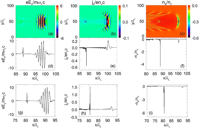
Figure 4. 2D simulations of ultrashort XUV pulse generation with a peak laser amplitude of aL = 10 and a pulse duration of 10TL , as well as a plasma density of ne /nc = 0.04 . Panels (a)–(c) show snapshots of the transverse electric field and the transverse current density along the laser polarization direction as well as the electron density when the incident laser is s-polarized. The transverse electric field, current density and electron density cuts on the laser axis are shown in panels (d)–(f). Panels (g)–(i) show the transverse electric field, current density and electron density cuts on the laser axis when the incident laser pulse is p-polarized.
Download figure:
Standard imageFor the case of p-polarization, the residual momenta of the trapped electrons in the y-direction are superimposed with the momentum components caused by the induced transverse electric field in the y-direction mentioned above. But the net electron current in the y-direction is still mainly due to the residual momenta since the other momentum components can cancel each other. Actually, the maximum net transverse current density near the axis in this case is about three times as high as that for the s-polarization, as shown in figure 4(h). Nevertheless, the XUV emissions are similar either in the peak amplitude or in the pulse duration for both cases, as shown in figure 6(a). Besides, it is worth emphasizing that the emission is observed preferably for the case when the spot size of the incident laser pulse is a few times larger than the plasma wavelength 2π /ωp , so that the wakefield structure is somehow similar to the 1D case. This means that it is different from the parameter regime ideal for bubble structure formation and electron acceleration [34, 35]. In the latter case, it is preferable that the laser spot size is comparable with the plasma wavelength.
Figure 5 illustrates the isosurfaces of the transverse electric fields and the electron density obtained from 3D simulation with the same laser and plasma parameters as in figure 4. It appears that the main features of the XUV emission are similar to those found in 2D simulation, even though there are still some differences in its peak current density, emitted pulse duration and frequency spectrum, as shown in the following.

Figure 5. Isosurfaces of the transverse electric fields (a) and electron density (b) from 3D simulation, where both the laser pulse and the produced XUV pulse (near x = 75λL ) as well as the corresponding electron density are shown.
Download figure:
Standard image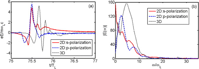
Figure 6. Electric fields of the emitted XUV pulses on the laser axis after propagating through plasma into vacuum (a) and the corresponding frequency spectra (b) obtained from 2D and 3D simulations. The parameters are the same as those in figures 4 and 5.
Download figure:
Standard imageFigure 6 displays a zoomed-in plot of the emitted XUV pulses and their spectra corresponding to figures 4 and 5. Compared with the 1D simulation results shown in figure 2, the peak amplitudes of the XUV pulses found in 2D/3D are over two times higher, but the durations are dozens of that from 1D simulation. Furthermore, their frequency spectra extend to about 35ωL , which is only about one-third bandwidth of that observed in 1D simulation. This can be attributed to the transverse effects arising from the transverse components of ponderomotive forces of the laser pulse as mentioned above. As a result, the magnitude of the density peak is higher and its spatial width is larger than those found in the 1D case. Furthermore, as the emission is caused by the density spike and residual electron momenta, it is strongly dependent upon the self-modulation of the laser pulse. In 2D and 3D geometry, the self-modulation of the laser pulse is also coupled with the self-focusing effect [20, 36], which is also different between 2D and 3D configurations. This can partially explain the difference in XUV emission between the 2D and 3D cases. Note that with the pump laser energy of about 23 J in the present 3D simulation, the produced XUV pulse energy can reach 9 mJ . The corresponding conversion efficiency is over 4 × 10- 4 .
5. Conclusions
We have shown theoretically and numerically that strong XUV radiation can be produced directly by laser wakefield excitation in the highly nonlinear regime in underdense plasma. It appears as short as a few hundreds of attoseconds in 1D simulations and as short as a few femtoseconds in 2D and 3D simulations. The high density spike of electron bunches trapped in the laser wakefield and the residual transverse momenta of electrons left behind the laser pulse are responsible for the XUV pulse emission, where the residual transverse momenta are caused by the front steepening of the laser pulse. In the 2D/3D simulations, XUV emission is found only near the laser axis with a much smaller spot size than the laser pulse. The XUV pulse emission can be observed in a wide laser and plasma parameter regime, typically with a laser intensity exceeding 1019 W cm- 2 and with a laser spot size larger than the plasma wavelength. This new mechanism provides a simple method for generating ultrafast intense XUV pulses. It may also provide a new diagnostic of the laser wakefields.
Acknowledgments
The authors acknowledge the OSIRIS Consortium, consisting of UCLA and IST (Lisbon, Portugal), for access to the OSIRIS 2.0 framework. This work was supported by the National Basic Research Program of China (grant number 2009GB105002) and the National Science Foundation of China (grant numbers 11121504 and 11075105). Numerical simulations were carried out on the Magic Cube at the Shanghai Supercomputer Center.