


Abstract
Based on trajectory calculations of xenon clusters up to ≈6000 atoms irradiated by laser pulses (peak intensities IM = 1014–1016 W cm−2, Gaussian pulse lengths τ = 10–230 fs and frequency 0.35 fs−1), we have analyzed the interrelation between outer ionization and ion kinetic energies. The following three main categories have been identified. (A) For short pulses (τ = 10 fs) of higher intensity IM = 1016 W cm−2, the outer ionization level leads to a sufficiently high positive cluster charge, which confines the remaining nanoplasma electrons to the cluster center. In this case, ion energies can be reasonably well accounted for by a multi-charge state lychee model, according to which outer ionization is vertical and the nanoplasma can be described by a non-expanding neutral cluster interior, causing a zero-energy component in the ion kinetic energy distribution and an expanding electron-free cluster periphery. (B) For a very low outer ionization level, which is realized for short pulses of low intensity (IM = 1014 W cm−2) and/or large clusters, a slow gradual evaporation of nanoplasma electrons under laser-free conditions on the picosecond time scale is observed, making the entire outer ionization process highly non-vertical despite the short laser pulse. Accordingly, ions are accelerated only by a gradual buildup of the total cluster charge. (C) For long pulses (τ = 230 fs), the cluster expansion during the laser pulse is large and outer ionization is non-vertical. The nanoplasma electrons attain high kinetic energies by resonance heating and are distributed over the entire ion framework without a neutral cluster interior. Consequently, a zero-energy component in the ion energy distribution is missing.
Export citation and abstract BibTeX RIS
1. Introduction
Rare-gas clusters are experimental and theoretical benchmark systems for investigating the interaction of ultra-intense femtosecond laser pulses with matter [1–3]. Insight into the underlying physical processes was gained, especially from particle trajectory simulations [4–23] and from particle-in-cell simulations [24–28]. For infrared (λ = 800 nm) pulses with peak intensities IM ⩾ 1014 W cm−2 the ionization of cluster atoms is triggered by a small number of tunnel ionizations (TI), followed by classical barrier suppression ionizations (BSI). The stripped electrons together with the ions form a nanoplasma and, driven by the external oscillating laser field, induce an avalanche of electron impact ionizations (EII). Depending on the pulse parameters (intensity and pulse length) and on the cluster size, the nanoplasma electrons are partly or completely removed from the cluster. The removal of nanoplasma electrons from the cluster is termed outer ionization as opposed to inner ionization [5], which subsumes the ionization channels of cluster atoms (TI, BSI and EII in this case).
Subsequently or parallel to the inner and outer ionization processes, Coulomb explosion (CE) sets in, converting the electrostatic repulsion of the cluster excess positive charges into ion kinetic energy up to the MeV region, depending on the cluster size and on the laser parameters. Thereby, the ion energetics and dynamics are strongly determined by the remaining nanoplasma electron population, which screens part of the positive charge in the cluster. In the case when the removal of nanoplasma electrons is complete before the cluster expansion sets in notably ('vertical complete outer ionization' [21]), so that the time scales of outer ionization and CE are separable, the description of the ion energetics and dynamics is quite simple and straightforward. Electrostatic models [29–31] are then applicable to the description of the dependence of the nuclear dynamics and energetics of CE on the cluster size, on the inner ionization level (expressed in terms of charge per atom) and on the pulse parameters (which determine the outer ionization level). The complete vertical ionization model will be transcended for larger clusters driven by lower laser intensities (IM ⩽ 1016 W cm−2), when novel features of incomplete outer ionization can be realized [21, 22]. For outer ionization electron dynamics the nuclear motion is not necessarily frozen, as outer ionization of large clusters driven by long (in the range of hundreds of femtoseconds) laser pulses occurs on the time scale of CE, precluding the separation of time scales between electron and nuclear dynamics. The electron-rich nanoplasma produced by incomplete outer ionization will manifest novel features of electron and nuclear dynamics. Under the conditions of incomplete outer ionization, the medium of the nanoplasma electrons is expected to provide a tool for the control of the CE energetics and dynamics, also with respect to inducing nuclear overrun effects during non-vertical ionization in two-pulse experiments and intracluster nuclear fusion [32].
We have carried out trajectory calculations for Xen clusters 55 ⩽ n ⩽ 6099 irradiated by infrared Gaussian laser pulses of peak intensities 1014 W cm−2 ⩽ IM ⩽ 1018 W cm−2 and pulse lengths 10 fs ⩽ τ ⩽ 230 fs, considerably extending the lower intensity limit of 1015 W cm−2 of our previous simulations [16–18, 21–22] toward lower intensities. For short pulses (τ ⩽ 30 fs) of low intensity, which is the regime of very electron-rich nanoplasmas, several experimental studies have recently been conducted [33–35]. The ion energetics over the entire considered cluster size and laser parameter ranges will be presented in a forthcoming publication; in this paper, we focus on intensities ⩽ 1016 W cm−2 and select three examples for which we discuss the interrelation between outer ionization and ion energetics. Most of the results emerging from our simulations of CE energetics pertain to classification of the effects of outer ionization dynamics and to extension of the electrostatic lychee model [14, 18, 21] to multiple charge states. A mechanistic issue for the ion energetics from an electron-rich nanoplasma pertains to the contribution from CE, which is determined by the conversion of the total potential energy, and from hydrodynamic expansion [36, 37], which is determined by the conversion of the electron kinetic energy into the kinetic energy of the ions.
2. Simulation method
We have previously described [16, 17] the molecular dynamics (MD) simulation scheme for high-energy electron dynamics in a cluster interacting with an electric and a magnetic field of a linearly polarized ultra-intense Gaussian laser pulse, with a photon energy of hν = 1.44 eV, a (cycle-averaged) peak intensity IM and a temporal length τ of the electric field envelope (the temporal full-width at half-maximum (FWHM) of the intensity profile being τ/√2). The laser electric field was taken as Fl(t) = FM exp[–4 ln(2)(t/τ)2] cos(2πνt + φ0) with a phase φ0 = 0 and FM being the electric field strength corresponding to IM [17]. In the MD simulations, the electrons are treated non-quantum mechanically but relativistically. This simulation scheme has been modified and extended in two respects.
Firstly, tunnel ionization (TI) has been incorporated using the Ammosov–Delone–Krainov (ADK) ionization probabilities [38]. The tunnel ionization probability wA of atom A per unit time was calculated by (in atomic units)
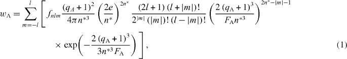
where n, l and m are the principal, angular and magnetic quantum numbers of the orbitals of the energetically uppermost electronic shell, qA the atomic charge before ionization,  the effective principal quantum number,
  the ionization energy of the atomic charge state qA in the absence of an electric field and FA the instantaneous local electric field at atom A consisting of the laser electric field, all the electrons and all other ions. Following the suggestion of Awasthi et al [39], the contributions of each orbital were multiplied by the corresponding orbital occupation numbers fnlm (0, 1 or 2). wA in equation (1) represents the non-cycle averaged tunnel ionization probability; wAċΔt is then the tunnel probability at atom A during the electronic MD time step Δt [40].
Secondly, the formalism of Fennel et al [15] was implemented to describe the enhancement of electron impact ionizations (EII) by the local electric field at each atom. In their treatment [15], the EII cross-sections are calculated by using the simplified Lotz formula [41]
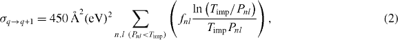
where Pnl and fnl are the ionization energies and the occupation numbers of the electronic subshells characterized by the principal and angular quantum numbers n, l and Timp is the impact kinetic energy of the impinging electron. According to Fennel et al [15], Pnl is taken relative to the electrostatic barrier rather than to the vacuum level. In our simulation scheme, Pnl was obtained by

with the corresponding ionization energy Pnl(0) in the absence of an electric field, the local electric field strength FA at atom A, the atomic charge qA + 1 after EII and the electron charge qe. For each charge state, the lowest ionization energy was taken from Cowan [42], higher ionization energies Pnl(0) were taken from scalar relativistic SCF-MP2 calculations as implemented in the MOLCAS 7.4 package [43], using a triple-zeta basis set contracted to a 7s6p4d2f1g form [44]. Timp is taken as the instantaneous electron kinetic energy corrected for the work to move it to the electrostatic barrier defined by the local electric field FA and the ion charge qA prior to EII

where  is the instantaneous position vector of the impinging electron with respect to the target atom.
The treatment of EII adapted from the work of Fennel et al [15] differs considerably from our previous work [16, 17], where we used experimental EII cross-sections that were fitted to the three-parameter Lotz formula [12, 41], but disregarded the enhancement of the EII cross-sections by the electric field. Although the Lotz formula in the form of equation (2) takes into account only the channel of direct EII, disregarding the excitation-autoionization and recombination-autoionization channels, which for some charge states can increase the EII cross-sections by one order of magnitude [45], the Lotz formula in the form of equation (2) has the advantage that cross-sections can be calculated for all charge states, whereas experimental EII cross-sections are available only until Xe11+ (as well as for some selected higher charge states). While in the previous simulations EII had to be disregarded for charge states higher than Xe11+, the inclusion of higher charge states is essential, because it is otherwise not possible to reproduce the ion charges as high as Xe20+–Xe23+ experimentally found already for intensities 1015–1016 W cm−2 [46, 47]. We considered a combined approach, taking experimental cross-sections for charge states up to Xe11+ and Lotz cross-sections in the form of equation (2) for higher charge states, but did not pursue it, because it is not known how the contributions from the excitation-autoionization and recombination-autoionization channels change under the influence of an electric field; the Lotz cross-sections, equation (2), are therefore considered a safe conservative choice. Although our simulations lead now for the Xe6099 cluster, IM = 1015 W cm−2, τ = 230 fs, to a maximum ion charge of 21, it is expected that the current treatment of EII still leads to too low charge states [15].
At every electronic time step, the local electric field at each atom is recalculated, consisting of the external laser electric field and the contributions from all the other ions and electrons, and each atom is checked for the occurrence of inner ionization in the hierarchy BSI > EII > TI, allowing only for one ionization per atom per time step. In this way, it is ensured, for instance, that tunnel ionization is applied only when the particular atom is not in the BSI regime where the ADK formula should not be applied [48]. Although the contribution of TI to the total number of inner ionizations is far below 1%, TI is essential for triggering the ionization avalanche at laser intensities below the BSI regime.
As the standard procedure, electrons farther away from the cluster center than ten cluster radii were removed permanently from the simulation. The initial MD setup consists of an fcc cluster structure of neutral atoms. We chose an electronic time step Δt between 10–4 and 10–3 fs; the nuclear time step was 20Δt.
3. Results and discussion
3.1. Simulation results
For three examples involving different cluster sizes and laser parameters, figure 1 shows time-resolved key quantities of the ionization process: the average ion charge qav, the number np of nanoplasma electrons per atom inside the cluster, the relative cluster radius R/R0 of the expanding cluster (taken as the distance of the most distant ion from the cluster center-of-mass, with R0 being the initial cluster radius) and, for a comparison of time scales, the oscillating laser electric field. The three examples represent three categories of incomplete outer ionization:
- (A)Vertical moderate outer ionization for short pulses, Xe1061, IM = 1016 W cm−2, τ = 10 fs (figure 1(a)). The nanoplasma electron population is in the range 1/2–3/4 of the average ion charge (np/qav = 0.73 in this example), and the cluster does not expand appreciably during the laser pulse. Depending on the cluster size, this category is found for moderate laser intensities 1015–1017 W cm−2.
- (B)Non-vertical low outer ionization for short weak pulses, Xe1061, IM = 1014 W cm−2, τ = 10 fs (figure 1(b)). Outer ionization is very low, only a few per cent of the average ion charge. Despite the negligible cluster expansion during the laser pulse, outer ionization is non-vertical, which will become apparent in the next section of this paper.
- (C)Non-vertical moderate to high outer ionization for long weak pulses, Xe6099, IM = 5 × 10¹⁴ W cm−2, τ = 230 fs (figure 1(c)). The cluster expansion during the laser pulse is large; at the end of the laser pulse, t ≈ τ, the cluster radius is increased by a factor of 10. For the long pulse of τ = 230 fs, outer ionization is very efficient via resonance heating [3, 49]. In this example, the cluster size and laser intensity were chosen such that the outer ionization level np/qav = 0.69 at the end of the trajectory is comparable to case (A). (As a general rule, outer ionization increases with increasing laser intensity and with decreasing cluster size.)

Figure 1. Time-resolved key quantities of the cluster ionization: the time-resolved average ion charge qav (closed line), the number np of nanoplasma electrons per atom (dashed line) and the relative cluster radius R/R0 with the initial cluster radius R0 (dotted line). The oscillating laser electric field (thin closed line) is given in arbitrary units. (a) Xe1061, IM = 1016 W cm−2, τ = 10 fs; (b) Xe1061, IM = 1014 W cm−2, τ = 10 fs; and (c) Xe6099, IM = 5 × 10¹⁴ W cm−2, τ = 230 fs. The examples given in panels (a)–(c) constitute outer ionization categories (A)–(C) discussed in this paper.
Download figure:
Standard imageBefore analyzing the ion kinetic energies, it is instructive to consider the total energy of electron-rich nanoplasmas. Figure 2 exhibits for the examples (A) and (B) the time-resolved total energy Etot of the entire system consisting of n ions and the total number nċne of electrons inside and outside the ionic framework (ne = np + noi, with noi being the number of electrons per atom outside the ion framework). Shown also is the partition of Etot, Etot = Tn + Te + Vtot, with Tn and Te being the ion and electron kinetic energy, respectively, and Vtot the total potential energy as the sum of ion repulsion, electron repulsion and ion–electron attraction. In both trajectory calculations all electrons were included; the standard procedure of removing distant electrons >10R (see section 2) was not applied. Etot is measured with respect to a total decomposition of the nanoplasma into single particles. Etot is not constant after the termination of the laser pulse due to the continued formation of ion charges and nanoplasma electrons by EII, as the expended ionization energy is not counted in this balance of Etot.
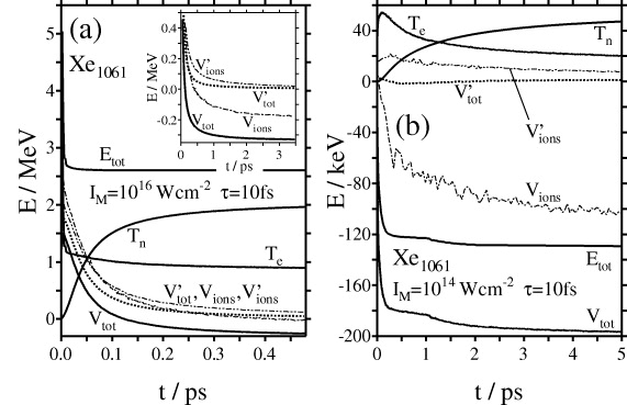
Figure 2. The time-dependent total energy Etot of the system consisting of n ions and nċne electrons inside and outside the ion framework, with respect to total decomposition of the nanoplasma into single particles, for outer ionization categories (A) and (B). Included are the total ion kinetic energy Tn, the total electron kinetic energy Te as well as the total potential energy Vtot; Etot = Tn + Te + Vtot, with Vtot = Vnn + Vee + Vne being the sum of the ion repulsion Vnn, electron repulsion Vee and ion–electron attraction energy Vne of the full ion charges and total number nċne of electrons. V'tot =V'nn +V'ee +V'ne is the corresponding potential energy of the effective ion charges and the remaining nne(free) free electrons. Vions and V'ions represent the sum of ion repulsion and attraction by the nanoplasma electrons, for the full ion charges and full number nċnp nanoplasma electrons, and for the effective ion charges and the number nnp(free) of free nanoplasma electrons, respectively. V'ions is the potential energy available for the ion acceleration. The inset in panel (a) shows Vtot, V'tot, Vions and V'ions with a better energy resolution and for longer times.
Download figure:
Standard imageIn the case (A) (figure 2(a)) Etot is positive, allowing in principle for a total decomposition of the plasma into single ions and electrons. The largest contribution to Etot at long times is the ion kinetic energy Tn. Another large part of Etot is carried away in terms of electron kinetic energy; more than 96% of the long-time Te value is attributed to electrons that were stripped by outer ionization. The total potential energy Vtot converges to a negative value despite the ongoing cluster expansion, indicating ion–electron trapping. Further analysis showed that 40% of all nanoplasma electrons remain trapped by ions at long times, orbiting the ions at distances rcut < 2 Å. Considering only the effective ion charges qi(eff) , i.e. the bare ion charges qi reduced by the number of trapped electrons, and the remaining n⋅ne(free) free electrons, the resulting potential energy V'tot (dotted line in figure 2) becomes positive and converges to zero at long times. (Regarding notation, we shall distinguish energies, which were calculated from effective ion charges and free electrons, by a prime.) Of particular interest is the potential energy V'ions which is available for the conversion into ion kinetic energy Tn. When the spatial charge distribution is spherical and the nanoplasma sufficiently diluted, V'ions is approximately given by (in atomic units)
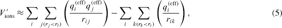
where k in the second double sum runs over all n⋅np(free) free nanoplasma electrons. For comparison, Vions is also included in figure 2, i.e. the corresponding quantity with the full ion charges qi and nċnp nanoplasma electrons. While the long-time value of Vions is negative, V'ions assumes a small positive value and goes to zero at long times, driving the ion acceleration.
In the case (B) (figure 2(b)) Etot converges to a negative value at long times; total decomposition of the nanoplasma into single particles is therefore precluded. Some 70% of the nanoplasma electrons were found to be trapped. V'tot and V'ions assume small positive values.
Another interesting issue of the energy analysis pertains to the question of the dominant driving force of the cluster expansion, CE or hydrodynamic expansion (HE), being attributed to the conversion of total potential energy and electron kinetic energy, respectively, into ion kinetic energy [36]. Under the condition that the total energy Etot of the system is constant in the course of the trajectory, the CE part is given by the difference ΔVtot = Vtot(tL) − Vtot(tI) of the total potential energy of the system and the HE part by the difference ΔTe = Te(tL) − Te(tI) of the electron kinetic energy, tI and tL being instants close to the beginning and at the end of the trajectory. In the ideal case, tI is chosen at a time when the inner ionization and energy absorption of the electrons has terminated and Etot has reached its final constant value. On the other hand, the kinetic energy attained by the ions at t < tI cannot be assigned to CE and HE, so that tI should be chosen as close as possible to the beginning of the trajectory. In practice, tI is a trade-off between both requirements. For the same reason, the energy analysis is not meaningful for long pulses (case (C)).
Table 1 contains the results of the analysis for examples (A) and (B). For the example (A) we chose tI = τ = 10 fs, when the nanoplasma build-up is nearly complete and the variation of the total energy in the course of the trajectory, Etot(tL) − Etot(tI) = 93 keV, is small compared to the final ion kinetic energy, Tn(tL) = 2079 keV. Also, at t = 10 fs the non-assignable part of the ion kinetic energy is still relatively small, Tn(tI) = 155 keV. With this choice of tI and tL, ΔVtot = 1702 keV and ΔTe = 317 keV, so that the relative contributions of CE and HE to the sum ΔVtot + ΔTe + Tn(tI) are 78 and 15%, respectively. The close agreement of the sum ΔVtot + ΔTe + Tn(tI) = 2174 keV with Tn(tL) = 2079 keV reflects the good accuracy of the energy partitioning. Clearly, example (A) pertains to the CE regime.
Table 1. Partitioning of the ion kinetic energy into contributions from CE and hydrodynamic expansion (HE), for the examples (A) and (B). tI and tL are the initial and the final instant of the trajectories, at which the kinetic, potential and total energies were taken for the energy analysis. ΔVtot = Vtot(tL) − Vtot(tI) and ΔTe = Te(tL) − Te(tI) represent the contributions from CE and HE, respectively; Tn(tI) is the initial ion kinetic energy that cannot be assigned to CE and HE. The relative contributions to the sum ΔVtot + ΔTe + Tn(tI) are given in per cent (in parentheses). If the energy partition were exact, then ΔVtot + ΔTe + Tn(tI) = Tn(TL); therefore the deviation of ΔVtot + ΔTe + Tn(tI) from Tn(TL) as well as the deviation of Etot(tL) − Etot(tI) from zero indicate the error of the energy partition.
| Example (A) | Example (B) | |
|---|---|---|
| tI (ps) | 0.010 | 0.112 |
| tL (ps) | 3.5 | 7.5 |
| ΔVtot (keV) | 1702 (78%) | 30 (44%) |
| ΔTe (keV) | 317 (15%) | 36.3 (53%) |
| Tn(tI) (keV) | 155 (7%) | 2.6 (4%) |
| ΔVtot+ΔTe+Tn(tI) (keV) | 2174 | 68.9 |
| Tn(tL) (keV) | 2079 | 49.8 |
| Etot(tL)–Etot(tI) (keV) | 93 | 20 |
The analysis of example (B) is fraught with much larger inaccuracies. Until t = τ, only 73% of the inner ionizations occur. We therefore chose tI = 112 fs; when Te becomes maximal, Etot(tL) − Etot(tI) drops to 20 keV and Tn(tI) = 2.6 keV is still relatively small. With this choice of tI one obtains ΔVtot = 30 keV and ΔTe = 36.3 keV, corresponding to contributions of 44% and 53% CE and HE, respectively. Although ΔVtot + ΔTe + Tn(tI) differs from Tn(tL) by 20 keV and Etot(tL) − Etot(tI) = 20 keV, indicating a large error of the energy partitioning which is 40% of Tn(tL), the trend is visible that a large, if not a major part of the cluster expansion, stems from HE.
Proceeding from an analysis of the total energy of the system to the individual ions, their long-time kinetic energies can, in principle, be obtained directly from a trajectory calculation. In practice, because of computational workload, trajectories are mostly not long enough, so that the potential energy residues have to be estimated. There are several methods for an energy correction:
- (1)A pairwise interaction formula based on V'ions , equation (5). The corrected energy Ti(corr) of ion i is given by its instantaneous kinetic energy Ti and the sum over all Coulomb interactions with the effective ion charges qj(eff) and free nanoplasma electrons k closer to the cluster center than ion i:

- (2)A central charge formula with effective ion charges. The energy correction for ion i is a single pairwise Coulomb term of the effective charge qi(eff) and a charge Qi in the cluster center, which is the sum of all the ion and electron charges closer to the cluster center than ion i:
- (3)The pairwise interaction formula, equation (6), with the full ion charges qi and the full number nċnp of nanoplasma electrons k:
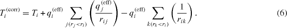


The energy correction corresponds to the potential energy Vions and was used in the previous work [21] where electron trapping was mostly insignificant.
Each of the three energy corrections presumes a spherical charge distribution inside the nanoplasma. In practical calculations, smoothed Coulomb potentials for the ion–electron and electron–electron interactions were used in equations (5), (6) and (9), in accordance with the trajectory calculations [9, 16–18, 21, 22].
The Xe1061 cluster is still small enough to check the three energy correction formulae against long-time ion kinetic energies, where Ti(corr) ≈Ti . For the outer ionization case (A), figure 3(a) shows the maximum corrected and uncorrected ion energy, EM and TM, respectively, as a function of time. The three correction formulae lead to nearly identical results and are nearly converged to the long-time TM value already at t = 200 fs. For the average ion energy (figure 3(b)), the values corrected by the pairwise interaction formula with effective ion charges and by the central charge formula are identical, converged already at t = 20 fs and in close agreement with the long-time 〈T〉 value. In contrast, the pairwise interaction formula without trapping gives too low values. The reason is that using bare ion charges in the energy correction formula (equation (9)) does not take into account the Coulomb repulsion between trapped electrons and other electrons which are closer to the cluster center. As the trapped electrons form a subsystem together with their host ion, the energy correction must involve all interactions of the subsystem with other ions and electrons. When the interparticle distances are large compared to the distances inside the ion-trapped electron subsystem, it suffices to reduce the ion charges rather than considering the repulsion of the subsystem electrons with other nanoplasma electrons explicitly. For the maximum ion energy (figure 3(a)), the pairwise interaction formula with bare ion charges and the full number of nanoplasma electrons (equation (9)) works well, because the maximum energy stems from an ion near the cluster surface, where trapping does not play a role for these laser parameters.
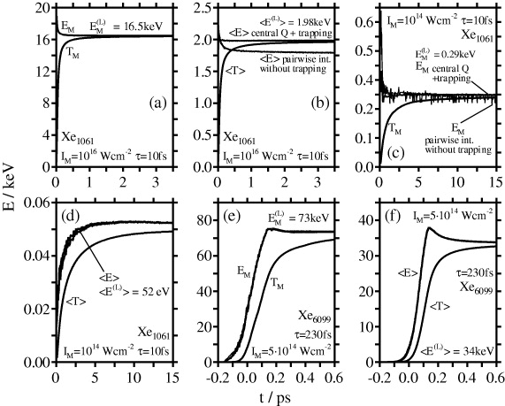
Figure 3. The time-dependent corrected and uncorrected maximum and average ion kinetic energies obtained from trajectory calculations. (a), (b) Xe1061, IM = 1016 W cm−2, τ = 10 fs (outer ionization category (A)). The three energy correction formulae, equations (6), (7) and (9), lead to undistinguishable curves EM, with the uncorrected maximum ion kinetic energy TM converging to the long-time corrected value EM(L) (panel (a)). For the average corrected ion energy 〈E〉 (panel (b)), the central charge formula and the pairwise interaction formula with trapping yield nearly identical results, with the uncorrected average kinetic energy 〈T〉 converging to their long-time value 〈E(L)〉, whereas the pairwise interaction formula without trapping gives too low values. (c), (d) Xe1061, IM = 1014 W cm−2, τ = 10 fs (outer ionization category (B)). The pairwise interaction formula and the central charge formula lead to nearly identical results for EM and 〈E〉. TM and 〈T〉 approach the long-time corrected values EM(L) and 〈E(L)〉 but are not converged until the end of the 15 ps trajectory. The pairwise interaction formula without trapping leads to unphysical fluctuations for EM (panel (c)) and to negative values for 〈E〉 (not shown in panel (d)). (e), (f) Xe6099, IM = 5 × 10¹⁴ W cm−2, τ = 230 fs (outer ionization category C). The three energy correction formulae give nearly identical results for EM and 〈E〉.
Download figure:
Standard imageIn all calculations an ion–electron cutoff distance of 2 Å was used; the ion energies turned out to be insensitive to the particular choice of the cutoff distance. The residence times of the trapped electrons increase with the dilution of the nanoplasma. A cursory analysis revealed that for the Xe1061 cluster irradiated by a pulse of IM = 1016 W cm−2, τ = 10 fs, the average residence time is of the order of 300–400 fs at t = 1 ps.
Figures 3(c) and (d) exhibit the maximum and the average ion energy for outer ionization category (B), the Xe1061 cluster irradiated by a laser pulse of IM = 1014 W cm−2, τ = 10 fs. The pairwise interaction formula with trapping (equation (6)) and the central charge formula (equations (7) and (8)) give nearly identical results for EM, whereas the pairwise interaction formula without trapping (equation (9)) results in unphysical fluctuations of EM (figure 3(c)). As equation (9) sums ion–electron interactions rk < ri, the number of summands oscillates with the instantaneous coordinates of the trapped electrons orbiting their host ion, indicating that for short weak pulses electron trapping plays a role also for surface ions. For the average ion energies (figure 3(d)), the pairwise interaction formula with trapping and the central charge formula converge to the same final value. The pairwise interaction formula without trapping (equation (9)) fails completely and gives negative average ion energies. Comparing the ion energetics of cases (A) and (B), not only the average and maximum ion energies are much lower in case (B). Rather, the striking difference lies in the slow convergence of ion energies, in particular of the average ion energy, in case (B). Whereas in case (A) the average ion energy is converged already at 20 fs after the temporal peak of the laser envelope function, in case (B) convergence is achieved only after ≈5 ps. This point will be analyzed in section 3.2 utilizing the lychee model.
In figures 3(e) and (f), the time-dependent maximum and average ion energies are presented for the example (C), the Xe6099 cluster irradiated by a 230 fs pulse at IM = 5 × 10¹⁴ W cm−2. The energies obtained by the pairwise interaction formula with and without trapping (equations (6) and (9)) and by the central charge formula (equations (7) and (8)) are nearly identical, as trapping is prevented by the high electron kinetic energies attained during resonance heating. The corrected average and maximum ion energies, 〈E〉 and EM, pass a maximum during the resonance of the nanoplasma electrons with the laser field (t = 140–180 fs). During the resonance, the electron population within the ion framework is lowered (cf figure 1(c)), so that the energy correction formulae overestimate the ion energies. After the resonance situation, the electrons are decelerated by the laser field and partly return from the vicinity of the cluster (<10R) into the ion framework. The ion energies are nearly converged at t ≈ τ, when the laser electric field has abated.
Our calculated single-trajectory results are in reasonably good agreement with the results of Holkundkar et al [23]. Their maximum ion energies for 25 fs infrared laser pulses are 7 keV for Xe2171 at IM = 1015 W cm−2 and 77 keV for Xe6100 at 2 × 10¹⁶ W cm−2; our results are 5.2 and 76 keV, respectively. For the Xe6100 cluster irradiated by a 125 fs pulse at IM = 1016 W cm−2, Holkundkar et al [23] obtained 〈E〉 = 58 keV and EM = 100 keV; our results are 〈E〉 = 56 keV and EM = 121 keV. For a Xe6140 cluster irradiated by a 100 fs pulse at IM = 1016 W cm−2, Petrov and Davis [13] have simulated an average ion energy of 68 keV, which is considerably higher than our value of 38 keV obtained for the Xe6099 cluster.
Erk et al [50] have recently published experimentally obtained ion kinetic energy distributions (KEDs) for xenon and argon clusters. To make contact with their experimental results, the simulated single-trajectory KEDs must be doubly averaged over the cluster size distribution and over the laser intensity profile [22]. For the cluster sizes we assume a log-normal distribution with an FWHM equal to the modal cluster size [51]. For the laser intensity we take a Gaussian beam intensity profile [52]

where IMmax is the spatially and temporarily overall peak intensity at the center of the focus volume, w0 the beam waist radius and zR = πw02 /λ is the Rayleigh length, with λ = 800 nm being the laser wavelength. The cluster beam, with a radius rB, is directed along the r-axis, which is perpendicular to the focus offset axis z. The relation between rB and zR determines which part of the intensity profile is relevant for intensity averaging. For rB ≫ zR, the averaging over the entire three-dimensional (3D) laser focus volume has to be carried out; for zR < rB, only a slice of the laser intensity profile around z = 0 is involved, so that equation (10) reduces to a 2D intensity profile

Compared to the 3D profile, in the 2D case the relative weight of low intensities is considerably lower. In the paper by Erk et al [50], rB = 0.75 mm, but zR is not specified. However, from experience zR can be assumed to be ≈2.5 mm [53], nearly realizing the 2D scenario of equation (11). The KEDs in the experiment of Erk et al were obtained for  and τ = 35 fs. For the double averaging in [22], we used ion energies from trajectories in the cluster size range 55 ⩽ n ⩽ 4093 and intensities 1014 W cm−2 ⩽ IM ⩽ 5 × 10¹⁵ W cm−2. Erk et al give KEDs for two average xenon cluster sizes, 〈n〉 = 200 and 700, which are in our simulated cluster size range. The experimental maximum ion energy for 〈n〉 = 200 is about 22 keV and for 〈n〉 = 700 27 keV. Applying the same definition of the maximum ion energy as in the experiment, that is, when the KED drops to the given fraction of its maximum value (2 × 10⁻⁴ for 〈n〉 = 200 and 4 × 10⁻⁵ for 〈n〉 = 700), the simulated maximum ion energies on the basis of a 2D intensity profile are 11 keV for 〈n〉 = 200 and 18 keV for 〈n〉 = 700. The corresponding maximum ion energies on the basis of the 3D intensity profile are much lower, 7 keV for 〈n〉 = 200 and 12 keV for 〈n〉 = 700. That is to say, all simulated values are considerably lower than the experimental values, but better agreement with the experiment is obtained for the 2D scenario. A more detailed analysis of the experimental KEDs will be given in a forthcoming paper. Trying to assess our simulation results for the ion energetics, one may expect in general that our trajectory simulation model tends to underestimate ion energies, since the neglect of the excitation-autoionization and recombination-autoionization EII channels (see section 2) causes too low ion charges. For 〈n〉 = 700, Erk et al observed a maximum charge state qM = 19, whereas our simulations give values qM = 13 for Xe1061 and qM = 14 for Xe2171 (IM = 5 × 10¹⁵ W cm−2, τ = 35 fs). The deviations between simulation and experiment may be partly due to the uncertainties of the experimental cluster size and laser intensity distributions. As pointed out by Schultze et al [54], the assumption of a Gaussian beam intensity profile is a significant oversimplification.
3.2. The multi-charge state lychee model
Insight into the ion energetics can be gained by using the electrostatic lychee model [14, 21]. The model presumes that (i) inner and outer ionizations are vertical, (ii) all nanoplasma electrons are confined to the cluster interior and form, together with the ions, a neutral sphere where the sum of ion and electron charges is equal, so that (iii) only ions in the electron-free cluster periphery participate in the Coulomb explosion. Knowing the initial radius R0 and the homogeneous initial density ρ of a spherical cluster, the lychee model gives analytical expressions for the central charge Q(r) as a function of the distance r from the cluster center, for the radius Rp of the neutral interior cluster sphere, for the ion energies E(r), for the average and maximum ion energies 〈E〉 and EM and for the ion kinetic energy distribution (KED) P(E) [21]. While in previous work [21] the lychee model was expressed for an average ion charge qav, an obvious improvement is extension to a charge distribution, in particular since EM and therefore the width of P(E) are determined by the maximum ion charge qM at the cluster surface. The extension to a multiple-charge state lychee model is straightforward, for simplicity presuming that the ions of each charge state are homogeneously distributed over the cluster with a density

where nq is the number of ions of charge q and n is the total number of ions. The resulting expressions for Rp, Q(r) and 〈E〉 are identical with those of the single-charge state lychee model (all energies in the equations are given in atomic units)


For the energy Eq(r) of an ion of charge q at a distance r from the cluster center, one obtains

and for the maximum ion energy

The energy distribution function P(E) is the superposition of the partial distribution functions Pq(E) of each charge state

with
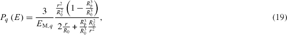
where EM,q = Eq(R0) is the maximum ion energy for charge state q; cf equations (16) and (17). The Pq(E) and, consequently, also P(E) are normalized to 1 − np/qav

excluding the neutral lychee core, which is consistent with the average ion energy 〈E〉, equation (15). Reasonably, one applies equations (12)–(20) to the effective ion charges and the free nanoplasma electron population rather than to the full ion charges and total nanoplasma electron population.
Applying the lychee model to the analysis of the slow convergence of the average ion energy in case (B), we note that the expression for 〈E〉, equation (15), contains powers of np/qav and qav2 in the prefactor. With x = np/qav and the average net charge per atom, qnet = qav − np, equation (15) can be recast:

To find out to what extent 〈E〉 is dependent on x = np/qav, in figure 4 the fractional polynomial in equation (21), which is equivalent to the relative average ion energy 〈E〉(x)/〈E〉(0) for constant qnet,

is plotted against np/qav. Note that 〈E〉(0) is the average ion energy for the lower limit np/qav = 0, when all nanoplasma electrons are trapped. The upper limit, np/qav = 1, where the total cluster charge is zero and 〈E〉(np/qav)/〈E〉(0) = 5/6, is approached by outer ionization category (B). Large clusters can come arbitrarily close to this limit. As shown by figure 4, the fractional polynomial, equation (22), varies at most by 17% over the entire np/qav range, so that 〈E〉 depends mainly on qnet. Since qnet is directly related to the total cluster charge Q(R0)

we conclude that the average ion energy depends mainly on the total cluster charge rather than on the charge distribution inside the cluster, and Q may be a key parameter for understanding the convergence behavior of the ion energetics and the underlying physical processes.

Figure 4. The fractional polynomial, equation (22), in the range 0 ⩽ x ⩽ 1, x = np/qav.
Download figure:
Standard imageFor the Xe1061 cluster, IM = 1016 W cm−2, τ = 10 fs (outer ionization category (A)), in figure 5 the central charge Q(i) (equation (8)) experienced by each ion i is plotted against the ion number i, where the ions are ordered according to their distance from the cluster center. In this way, figure 5 contains information on the charge distribution inside the cluster as well as on the total cluster charge; Q(1061) represents the central charge experienced by a surface ion. Q(i) is given for t = 0.02, 0.5 and 3.5 ps. For all the considered times, Q(i) reflects a typical spatial lychee charge distribution, low Q values in the cluster interior and a steep rise toward the cluster periphery. Q(1061) is practically converged at t = 0.5 ps. At t = 20 fs, when 〈E〉 is already converged but EM still by 1.5 keV above its final value of 16.5 keV (figure 3(a)), Q(1061) exceeds its final value by 20%. Apparently, the lowering of Q(1061) for t > 20 fs is due to the rapid expansion of the cluster periphery into the surrounding electron cloud.
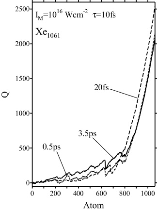
Figure 5. The central charge Q(i), equation (8), experienced by the ions of the Xe1061 cluster irradiated by a laser pulse of IM = 1016 W cm−2, τ = 10 fs (outer ionization category (A)), calculated from trajectory data. The 1061 ions i defining the abscissa are ordered by their distance from the cluster center, so that Q(i) reflects the spatial charge distribution in the cluster; Q(1061) is the central charge experienced by a surface ion. Q(i) is given at times t = 0.02, 0.5 and 3.5 ps.
Download figure:
Standard imageFor the outer ionization category (B), the spatial dependence and time evolution of Q(i) are very different from that of category (A). In figure 6(a), the Q(i) function is given for t = 0.02, 0.2, 1, 5, 10 and 15 ps. Q(i) assumes much lower values than in case (A) and is not converged until at least t = 10 ps. To elucidate the different roles of ions and electrons, in figure 6(b) Q(i) is calculated from the reduced ion charges only, i.e. excluding the free nanoplasma electrons. When the free nanoplasma electrons are excluded, not only are the Q(i) values much higher, as expected, but Q(i) also converges much faster. This provides additional evidence that the slow convergence of the total Q(i) function (figure 6(a)) is caused by a gradual loss of nanoplasma electrons, a continuous evaporation of nanoplasma electrons from the ion framework on the picosecond time scale. The consequence of the slow electron evaporation on the ion energetics is that the ions are accelerated by a variable central charge Q, precluding a meaningful estimate of the ion potential energy residues from short trajectories. The electron evaporation causes the outer ionization to be highly non-vertical, despite a negligible cluster expansion during the short laser pulse. A comparison of figures 3(d) and 6(a) shows that 〈E〉 is earlier converged (around t = 5 ps) than Q (not before t = 10–15 ps), reflecting that the effect of the electron evaporation on the ion energetics fades away at a late stage of the cluster expansion.
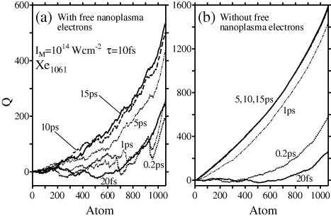
Figure 6. The central charge Q(i) experienced by the ions of the Xe1061 cluster irradiated by a laser pulse of IM = 1014 W cm−2, τ = 10 fs (outer ionization category (B)), at times t = 0.02, 0.2, 1, 5, 10 and 15 ps, calculated from trajectory data. (a) Q(i) calculated from ion and electron charges; (b) Q(i) calculated from effective ion charges without the contribution of the free nanoplasma electrons.
Download figure:
Standard imageFor a quantitative comparison of the KEDs from the trajectory calculations and those of the lychee model, it must be taken into account that in the trajectory calculations, P(E) is approximated by a histogram hk of ion energies of finite-energy intervals ΔE

Unlike in the lychee model, in the trajectory calculations P(E) is normalized to 1, as well as the ions in the nearly neutral lychee core participate in the cluster expansion and contribute to the hk of the lowest-energy interval. Therefore, to be comparable with the KED of the trajectory calculation, the constant term np(free) /qav(eff) δ k has to be added to h0 of the lychee model

The last term in equation (25), n0/n(1 − np(free) /qav(eff) ) ⋅ δ k,/ accounts for ions that have reached charge neutrality by trapping the corresponding number of electrons, with n0 and n being the number of neutral atoms and the total number of atoms in the cluster, respectively.
For a numerical application of equation (25), with Plychee(E) from equations (18) and (19), np(free) and the ion charge state abundances  are taken from trajectory calculations. The question arises then at which instant of the trajectory, np(free) and
  should be taken, as the charge build-up in the cluster is not completely vertical even for outer ionization case (A). One possible choice is at a comparatively long time tL of the trajectory, when the ion energies are converged. A better alternative seems to be the charge distribution, which is dominant for the cluster expansion; we therefore take np(free) and
  at the instant tacc when the average ion acceleration reaches its maximum, tacc = 20, 200 and 110 fs for examples (A)–(C), respectively. For the example (A) the instant t = 20 fs practically coincides with the termination of outer ionization. In case (B), the delay of tacc to 200 fs, which is long after the termination of the laser pulse, reflects the slow charge build-up in the cluster by electron evaporation. In case (C), the instant of maximum ion acceleration coincides roughly with the enhanced outer ionization at the nanoplasma electron resonance.
Figure 7 shows the distributions of effective and bare ion charges at the maximum ion acceleration times tacc. For comparison, the corresponding ion charge distributions at long times tL have been included. Using the abundances of effective ion charges and free nanoplasma electron populations at tacc, the KEDs calculated by the lychee model are shown in figure 8, together with the corresponding results of the trajectory calculations.
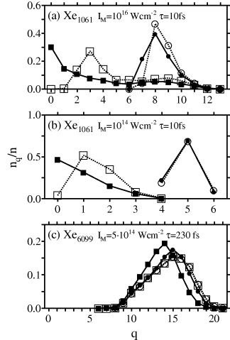
Figure 7. The relative ion charge state abundances for the examples (A)–(C). Symbols ▪ and □ are the effective ion charge state abundances nq(eff) /n at t = tacc and t = tL, respectively;  and
and  are the full ion charge state abundances nq/n at t = tacc and t = tL, respectively. For the examples (A)–(C), the times tacc are at 20, 200 and 110 fs (times when the average ion acceleration assumes a maximum), and the times tL are 3.5, 15 and 0.6 ps, respectively.
Download figure:
Standard image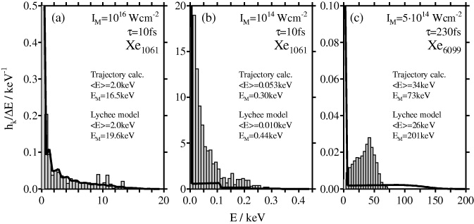
Figure 8. The KEDs for the examples (A)–(C), approximated by the histogram values hk/ΔE for finite-energy intervals ΔE. The KEDs obtained from the trajectory calculations are represented by histograms. The lychee model results were obtained from equation (25), using the effective ion charges and populations of free nanoplasma electrons at t = tacc. The trajectory and lychee model results for 〈E〉 and EM are given inside the panels.
Download figure:
Standard imageIn case (A) (figure 8(a)), the KEDs of the trajectory calculation and of the lychee model are in overall good agreement and the average ion energy is in perfect agreement. The overestimate of EM by the lychee model by 3 keV is a non-vertical effect, as the cluster expansion sets in before the charge build-up is complete. The low-energy component h0, which constitutes the maximum of the KED, is reproduced by the lychee model within 35%.
The underlying effective ion charge abundances of case (A) (figure 7(a)), at tacc = 20 fs and tL = 3.5 ps, differ mainly for the low ion charges 0–4, whereas the highest ion charge q = 13, which defines the width of the KED, is practically unaffected. Effective ion charges of 0 and 1 are a consequence of the high electron density in the practically unexpanded lychee core at tacc = 20 fs; under these conditions, electrons are only formally assigned to ions according to their ion–electron cutoff distance (2 Å) rather than actually trapped. (Ions that formally acquire negative charges by close encounters with electrons are counted as neutral atoms; the resulting excess electrons are counted as free nanoplasma electrons.) Using the ion charge abundances at tL = 3.5 ps, where the effective ion charges of 0 and 1 are missing, the lychee model gives nearly identical results, 〈E〉 = 1.92 keV and EM = 19.6 keV, and a very similar KED (not shown in figure 8(a) for t = tL), provided that the number of nanoplasma electrons is chosen such that Q(1061) is adjusted to the same value as that at t = tacc. Note that Q(1061) at t = tL is lower by almost 500 charge units than that at t = tacc (figure 5) due to the rapid expansion of the cluster periphery into the surrounding dilute electron cloud. While the reentry of the electrons into the expanded cluster periphery has a relatively small effect on the ion energetics of the trajectory, the 500 charge units make a considerable difference to np(free) as one of the key input parameters of the lychee model; the inclusion of the 500 electrons lowers 〈E〉 and EM to 1.25 and 15.9 keV, respectively. In conclusion, the lychee model results for 〈E〉 and EM are insensitive to the abundances of low ion charges, as long as the total cluster charge and the highest ion charge remain unaffected, reflecting the essence of equations (17) and (21).
The ion charges are not homogeneously distributed over the entire cluster as presumed by the lychee model. Rather, higher ion charges are enriched toward the cluster periphery. The presumption of a spatially homogeneous distribution of ion charges does not affect EM but is expected to influence the shape of the KED. In particular, the larger number of higher charge states in the cluster periphery will enhance the high-energy tail of the KED.
Proceeding to case (B) (figure 8(b)), the deviations of the lychee model results manifest extreme non-vertical effects. With the abundances of reduced ion charges and the number of free nanoplasma electrons taken at tacc = 200 fs, the lychee model underestimates 〈E〉 by a factor of 5. To reproduce the trajectory calculation result of 〈E〉 = 53 eV, the lychee model requires a central charge value Q(1061) of ≈420, which is approached only at t ≈ 4–5 ps (cf figure 6(a)), when 〈E〉 of the trajectory calculation also converges. In view of this slow charge build-up, it is therefore at first surprising that the lychee model overestimates EM. Taking the maximum effective ion charge qM(eff) = 4 (figure 7(b)), the lychee model yields EM = 0.44 keV as compared to EM = 0.33 keV from the trajectory calculation. However, a closer inspection of the trajectory reveals that although the maximum effective ion charge of 4 is reached already at an early stage of the trajectory, it is not constantly attributed to the same ions. Short-time averaging shows that the maximum ion charge fluctuates between 2 and 4, reaching its final constant value of 4 only at t ≈ 0.5 ps. The shape of the KED calculated by the lychee model is dominated by the low-energy component h0, which is by one order of magnitude higher than that of the trajectory calculation. In the trajectory calculation, the sharp h0 peak is spread over a larger number of low-energy intervals, reflecting the large departure of the spatial charge distribution (figure 6(a)) from that of a lychee structure.
In case (C) (figure 8(c)), the EM value calculated by the lychee model is 201 keV, being too high by almost a factor of 3, as a consequence of the neglect of the large cluster expansion until tacc, R(tacc) = 8R0 (figure 1(c)). Furthermore, the lychee model predicts a large low-energy component h0 of the KED, since the lychee model presumes all nanoplasma electrons to be located in the lychee core due to the neglect of electron dynamics. A neutral cluster core is not found in the trajectory calculation, as the electrons are nearly equally distributed over the entire ion framework by resonance heating.
For carrying out trajectory calculations, it is of practical interest to define some guidelines on what is the temporal length of a trajectory that is necessary for achieving convergence of the ion energies. From the foregoing discussion one can infer that a sufficient criterion for the convergence of the corrected ion energies is the convergence of the charge distribution inside the cluster and of the total cluster charge. This includes the absence of nuclear overrun subsequent to the truncation of the trajectory, as nuclear overrun can lead to an exchange of ion energies. However, as examples (A) and (B) have shown, the effect of the remaining variations of the charge distribution on ion energies fades out at a late stage of the cluster expansion, so that the criterion of a converged charge distribution is sufficient but not necessary. As an empirical rule of thumb, we found that the corrected ion energies are sufficiently converged when 〈T〉/〈E〉 ⩾ 0.85.
4. Conclusions
The inclusion of tunnel ionization and of the enhancement of EII by the electric field [15] in the simulation formalism allowed us to consider laser peak intensities down to IM = 1014 W cm−2, one order of magnitude lower than that in our previous simulations [21, 22]. A presentation of the ion energetics over the entire pulse parameter range considered, IM = 1014–1018 W cm−2, τ = 10–230 fs, and a comparison with our previous simulation results and with experimental results will be given in a forthcoming paper. From these results, we mention here only that we did not find anomalous anisotropy of the ion energies recently reported by Skopolová et al [33] and Mathur et al [34, 35], according to which higher ion energies have been found experimentally perpendicular to the laser polarization direction. In our simulations we found higher ion energies in the laser polarization direction. With decreasing the laser intensity and with decreasing the pulse length, the average ion energy becomes increasingly isotropic except from some fluctuations.
In this paper, we have selected three examples to discuss the dependence of the ion energetics on outer ionization. These three examples represent three categories of incomplete outer ionization, resulting in electron-rich nanoplasmas: (A) vertical incomplete outer ionization for short (τ = 10 fs) intense (IM = 1016 W cm−2) pulses; (B) non-vertical incomplete outer ionization for short (τ = 10 fs) weak (IM = 1014 W cm−2) pulses; and (C) non-vertical incomplete outer ionization for long (τ = 230 fs) weak (5 × 10¹⁴ W cm−2) pulses. While cases (A) and (C) have already been identified in previous work [21], case (B) is new. In case (C), the non-verticality of outer ionization is caused by the large cluster expansion during the long laser pulse; the cluster charge build-up ends with the termination of the laser pulse. In contrast, in case (B) the cluster expansion during the short laser pulse is negligible, but the cluster charge build-up continues by electron evaporation under laser-free conditions for a long time.
The example representing outer ionization category (A) differs from example (B) only by the higher laser intensity and consequently by a higher outer ionization level, better confining the remaining nanoplasma electrons to the cluster interior and prohibiting electron evaporation. Likewise, one may expect that increasing the cluster size causes a transition from outer ionization category (A) to (B), due to a decreasing outer ionization level for larger clusters. A quantification of the cluster size and intensity dependence of the vertical to non-vertical transition will be of interest.
To improve the description of the ion KED function by the electrostatic lychee model, we have extended the model to multi-charge states. In the case of vertical outer ionization (example (A)), the model reproduces the energy distribution function semiquantitatively. The characteristic signature of a lychee core is its intense low-energy peak in the ion kinetic energy distribution. Such low-energy peaks are exhibited in the ion kinetic energy distributions of Erk et al [50], which deserve further analysis. In case of non-vertical outer ionization by short pulses (example (B)), the lychee model shows very poor numerical agreement with the simulation results but was very useful in interpreting and characterizing the underlying physical processes. In the case of non-vertical outer ionizations by long pulses (example (C)) the lychee model fails completely due to the total neglect of the electron dynamics. Clearly, a further improvement of the lychee model requires a smooth rather than an abrupt transition between the neutral lychee core and the electron-free cluster periphery via the electron kinetic energy governing the spatial electron distribution inside the ion framework.
Acknowledgments
We are grateful to Professor Uzi Even for discussions of the laser-intensity profiles. Computation time, technical and manpower support of the computation center IZO-SGI SDIker of the University of the Basque Country (UPV/EHU), provided by the Spanish Ministry of Science and Education (MICINN), by the Basque Government (GV/EJ) and by the European Social Fund (ESF) are gratefully acknowledged. This research was partially supported by the Saiotek Program (GV/EJ).