


Abstract
The quantum Wigner function of an electron scattered by an ion in a strong laser field is considered in the framework of a one-dimensional scattering model with a soft-core Coulomb potential. The Wigner function contains much more information on the scattering process than the projected probability distributions in position and momentum space considered previously. The formation of the above-threshold ionization (ATI) energy spectrum, including ATI peaks, modulations and transients, can be easily explained by using the interference of phase-space trajectories.
Export citation and abstract BibTeX RIS
1. Introduction
Electron–ion scattering in strong laser fields is of fundamental importance in the process of strong field ionization of atoms [1, 2]. The rescattering of the electron after ionization gives rise to scattering rings in the angular distribution [3] and to a plateau region in the energy distribution [4] in high-order above-threshold ionization (ATI). Laser-driven electron–ion scattering also plays an important role for inverse bremsstrahlung absorption of laser light in plasmas [5–8]. Numerical solutions to the time-dependent Schrödinger equation (TDSE) provide detailed information on the spatial probability distribution as well as the energy and momentum distributions of the scattered electrons [9]. However, while the energy distribution shows regular ATI peaks separated by one-photon energy, the spatial distributions apparently miss a simple physical interpretation. It is only in some cases that spatial wavepackets have been successfully identified with classical electron orbits [10].
In order to gain a better understanding of the position–momentum correlations of the scattered electrons, it is worth studying the evolution of the scattering problem in the joint phase space. Although phase-space trajectories are excluded in quantum mechanics by the Heisenberg uncertainty relation, a generalized phase-space representation of a quantum system can be given in terms of the Wigner function [11]. The Wigner function represents a quasi-probability distribution function, assuming positive and negative values, which approaches the usual phase-space probability distribution in the classical limit. In the context of strong-field laser–atom interactions, the Wigner function has apparently been studied only occasionally to visualize, e.g., stabilization [12], tunneling [13] and double ionization [14].
In this work, we calculate the Wigner function numerically from the underlying quantum Liouville equation to study its evolution during the scattering of an incident electron beam by an ion over several periods of the applied laser field. We focus our attention on the scattering by a 1d soft-core Coulomb potential in the presence of a linearly polarized laser field. Basic strong-field features of ionization [15, 16] and scattering [17, 18] have already been studied in this framework. Here we generalize previous work by considering the evolution in 2d phase space based on a fast Fourier transform (FFT) split operator method. It will be shown that the phase-space trajectories of the scattered electrons indicate both classical and nonclassical features and that the observed position–momentum correlations provide further insight into the formation of ATI spectra.
2. Basic equations
The evolution of the statistical operator ρ(t) of a quantum system with the Hamilton operator H is governed by the von Neumann equation

Here and in the following, atomic units are used, where the electron mass, the elementary charge and the Planck constant are equal to unity (m = e = ℏ = 1). We consider a 1d scattering model with the Hamiltonian

The scattering potential is taken as a soft-core Coulomb potential

In ionization problems, the parameter  is often taken in the range ⪆1. For = 1.4 the ground state energy of the model potential assumes approximately the value −0.5 of hydrogen. However, for typical impact velocities of the order of unity the potential varies relatively slowly and its reflectivity therefore is quite small. In scattering problems, it is therefore useful to consider the parameter regime
  . In the present calculations we have set = 0.1, which accounts for about 10% reflection at impact velocities of the order of unity [17].
The interaction with the laser field is described in the Kramers–Henneberger (KH) framework [19]. In an oscillating laser field,  , an electron is subject to the quiver motion

In the KH frame, the quiver motion is removed and, instead, the scattering potential in (2) is oscillating as U = U(x + ξ(t)). The KH frame is convenient, since the asymptotic velocities for |x| → ∞ correspond to the drift velocities of the particle measured outside the laser field.
The initial wavefunction for an incident electron is chosen as a Gaussian wavepacket,

The probability distribution of x is w(x) = |ψ(x)|2. It is normalized to unity. The expectation values for position and momentum are x0 and p0, respectively, and the standard deviation of x from x0 is σ.
The Wigner function is defined in terms of the density matrix 〈x|ρ|x'〉 by a coordinate transformation x = q + r/2, x' = q − r/2 and a Fourier transformation with respect to the difference coordinate r,

By definition, the Wigner function is real; however, in contrast to a classical phase-space distribution function it can assume negative values. The Wigner function of (5) is a Gaussian probability distribution with respect to both p and q,

being normalized according to

According to (1) and (6), the Wigner function satisfies the quantum Liouville equation

with the Liouville operator

The Liouville equation of classical mechanics is obtained by expanding the potentials up to linear order around q.
The Liouville equation (9) has been solved numerically by an FFT-split-operator method similar to those used in [20–22]. For a sufficiently small time step, Δt = tn+1 − tn, the Wigner function can be propagated by the time-evolution operator

The Liouville operator can be split into parts,  , which include only position or momentum derivatives,

Up to second order in Δt, the time-evolution operator can then be factorized in the form

with

Applying alternating Fourier transforms with respect to q and p, each factor of (13) can be reduced to a simple multiplication operator. For N time steps it is sufficient to perform first one half-step with Uq(Δt/2), then N full-steps with the product Uq(Δt)Up(Δt) and finally one half-step backwards with Uq(−Δt/2). In our calculations the time step was chosen as Δt = 0.01 and phase-space grids with 2048 or 4096 points in each direction have been used. The separation of grid points was approximately 0.1 in the q-direction and 0.01 in the p-direction, which proved to be sufficient for resolving all interference fringes with appreciable visibility.
3. Interference of phase-space trajectories
To gain a physical understanding of the Wigner function of the scattered wavepacket, it is helpful to first consider simple superpositions of quantum states and their interference patterns in phase space. Let |ψ〉 = c1|k1〉 + c2|k2〉 be a superposition of two momentum eigenstates. The wavefunction in the position representation is

and the Wigner function of the corresponding density matrix 〈x|ρ|x'〉 = ψ(x)ψ*(x') is found to be

The first two terms correspond to classical streams with definite momenta k1 and k2. The third term is a nonclassical contribution that corresponds to the quantum interference in the spatial probability distribution. It varies along the q-direction with the difference wavenumber k1 − k2 and it propagates with the mean wavenumber (k1 + k2)/2. This example shows nicely how the Wigner function contains both classical particle properties and nonclassical wave properties being resolved in phase space by their different momenta.
In the semiclassical framework, the plane waves can be generalized with the Wentzel-Kramers-Brillouin (WKB) approximation to WKB waves with local wavenumbers k1,2(q). A pair of branches can be continued up to a common turning point where they merge with a vertical slope. The generic behavior of the Wigner function of a superposition of momentum states is two branches originating from a turning point with vertical slope and enclosing on the concave side an interference pattern with the local wavenumber k1(q) − k2(q) centered at the mean momentum (k1(q) + k2(q))/2. For instance, figure 1 shows the Wigner function of the wavefunction

with local wavenumbers  in the half-space x < 0. It represents an approximation to the stationary state with energy E = 0 in a linearly increasing potential V (x) = x/2. For simplicity the amplitudes are taken constant and a constant phase π/4 has been neglected. The well-known exact wavefunction can be expressed in terms of the Airy function Ai(x).
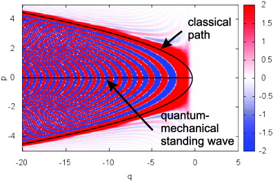
Figure 1. Wigner function of the wavefunction (16), consisting of an incident and a reflected WKB wave with position-dependent momenta  , respectively. The Wigner function shows the classical branches p = k1,2(q), merging at the turning point (p = 0, q = 0), and the quantum interference pattern, originating from the standing wave with momentum p = (k1 + k2)/2 = 0.
Download figure:
Standard imageAnother important example is a superposition of two position eigenstates |ψ〉 = c1|x1〉 + c2|x2〉. A position eigenstate is a simple model of a particle localized at a definite position with a corresponding wide spread in momentum. In the momentum representation, the wavefunction becomes

The Wigner function can now be calculated from the density matrix in the momentum representation 〈k|ρ|k'〉 = ψ(k)ψ*(k') by setting k = p + s/2, k' = p − s/2 and taking the inverse Fourier transform
It consists of the populations at the positions x1,2 and an interference pattern at the mean position (x1 + x2)/2 varying along the momentum direction with the wavenumber x1 − x2. Generalizing again the plane waves to the WKB waves, two branches with local wavenumbers x1,2(p) merging at a turning point with horizontal slope will enclose an interference pattern with local wavenumber x1(p) − x2(p) along the p coordinate. Schematically, the Wigner function has the same form as in figure 1 with q and p interchanged. The interference pattern along the p-direction is of particular interest, since it determines directly the momentum and energy spectra.
Basic properties of ATI spectra can simply be understood from this picture. First, consider jets of particles that originate from scattering at the ion in subsequent periods of the laser field. The particles with a given momentum p will be found at time t at the positions xn(p) = p(t − nT), where n = 0,1,2,... denotes the laser cycle of the emission and T = 2π/ω the laser period. The interference pattern between neighboring branches xn(p) and xn+1(p) is directed along the p-direction and has the wavelength Δp = 2π/(xn − xn+1) = ω/p. In the energy spectrum, corresponding peaks occur at the distance

As a conclusion of this simple argument, one obtains the familiar ATI peaks, separated by the photon energy.
There is another interference pattern in ATI spectra that is associated with the particles scattered within one period. Neglecting for simplicity the drift motion, the backscattered particles are emitted at time ts with the momentum p = −2v0 cos(ωts) at the position x = ξ0 sin(ωts) in the KH frame. The phase-space trajectory of the ensemble of emitted particles is given by

On the x-axis, v = 0, the ellipse has the width 2ξ0. From this width one can estimate the period of the momentum spectrum inside the ellipse as Δp = 2π/(2ξ0) = π/ξ. Accordingly, the ATI peaks in the energy spectrum will be modulated with a period of approximately

In contrast to the constant separation of the ATI peaks (19), the modulational wavelength (21) depends on the quiver amplitude and increases with momentum.
Finally, we consider the Wigner function for a superposition |ψ〉 = c1|x0〉 + c2|p0〉 of position and momentum eigenstates. It describes the interference of free and bound parts of the wavefunction. The density matrix is given by

Taking the Fourier transform with respect to the difference coordinate r = x − x' yields the Wigner function

It shows hyperbolic interference fringes n = 0,1,2,... at the positions (p − p0)(q − x0) = nπ + const.
4. Scattering by the 1d soft-core Coulomb potential
We first focus our attention on the scattering of a Gaussian wavepacket (x0 = −50, p0 = 1,  ) by a soft-core Coulomb potential in the absence of a laser field. Looking at this simple example, one can clearly recognize the classical and nonclassical features of the Wigner phase-space representation. In figure 2, the Wigner function is presented at different stages of the scattering process. Red color corresponds to positive and blue color to negative values of the quasi-probability. At time t = 10, the initial distribution has become slightly sheared due to the different distances moved by particles with different momenta, but it appears closely classical. At time t = 30, the center of the wavepacket has moved to x = −20 and the front has reached the scattering center at x = 0. Within the interaction region, the distribution becomes nonclassical. The population localized within the range of the potential interferes with the incoming beam, leading to hyperbolic fringes as in (23). At time t = 50, the center of the Gaussian has reached the scattering center. In the upper half-space (p > 0) one can recognize the quasi-classical behavior of particles crossing the potential with a given energy, thereby gaining momentum near the scattering center. In addition, nonclassical hyperbolic fringes arise from the incoming and transmitted beams interfering with the localized distribution around x = 0. In the lower half-space (p < 0) the distribution is dominant in the region q < 0 of the reflected wave. Along the negative q-axis one can recognize the interference pattern between the incoming and reflected waves in accordance with (15). At later times (t = 90), the incident packet has passed the scattering center and becomes spatially separated from the reflected one. Within the scattering region the distribution becomes rapidly oscillating in both the p- and q-directions. Due to the rapidly varying phase, the projected position and momentum probability distributions average to zero in this region, although the amplitudes of the Wigner function are still appreciable at the final time. This suggests that the spatial wavepackets decay after the interaction predominately by phase averaging of the Wigner function along the momentum direction.

Figure 2. The Wigner function of a Gaussian wavepacket (x0 = −50, p0 = 1,  ) scattered by a soft-core Coulomb potential ( = 0.1) in the absence of a laser field.
Download figure:
Standard image5. Laser-driven scattering
We now consider laser-driven scattering in a laser field with amplitude  and frequency ω = 0.2. The impact velocity (p0 = 2) is chosen larger than the quiver velocity (v0 = 1) to prevent the minimum collision velocity p0 − v0 from becoming small or negative. Furthermore, the laser period is larger than the typical duration of the collision (ω/v0 = 0.02 ≪ 1). These parameters correspond to the regime of instantaneous collisions [17]. If the duration of the interaction is much smaller than the laser period, the laser field is approximately fixed during the collision. Therefore the basic effect of the laser field consists in the modulation of the impact velocities of the Coulomb collision. From instantaneous collision models one expects backscattered particles with momenta p = −p0 − 2v0 cos(ωts), depending on the time ts of the collision.
The evolution of the Wigner function of a Gaussian wavepacket (x0 = −75, p0 = 2,  ) is shown in figure 3. The period of the laser field is T = 2π/ω ≈ 31. Within the first period the magnitude of the velocity of the scattered particles decreases from p0 + 2v0 = 4 to p0 − 2v0 = 0 (t = 10) and increases again to 4 (t = 20,30). The corresponding phase-space curve is indicated in the figure as the classical path of backward scattered particles. The two branches formed within the first and the second half-cycle interfere. One can already recognize transient interference fringes (denoted as momentum maxima) that evolve later to the ATI spectrum (19). Within the second period (t = 40, 50, 60) this process is repeated. The modulation of the phase-space curve by the quiver motion as indicated schematically in (21) now becomes clearly visible (denoted as modulation maxima). Within the area enclosed there appear the interference fringes that cause the modulation of the energy spectrum. After the third period (t = 90: left panel) one can observe three emitted classical jets with corresponding areas of nonclassical interference patterns. In the forward direction, the beam is periodically bunched by accelerated and decelerated particles (t = 90: right panel). The interference pattern (momentum maxima) produced between subsequent bunches corresponds to the ATI peaks in the forward peak of the energy spectrum (figure 4).
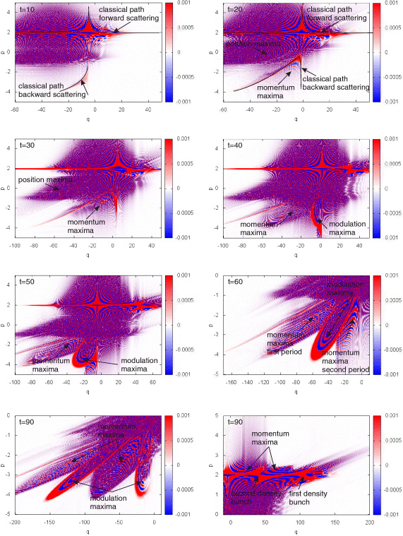
Figure 3. Scattering of a Gaussian wavepacket (x0 = −75, p0 = 2.0,  ) by a soft-core Coulomb potential ( = 0.1) in the presence of a laser field (ω = 0.2,
  ).
).
Download figure:
Standard image
Figure 4. Energy spectra at different times indicating transient interference fringes between bound and free parts of the wave after the first period (t = 30), the appearance of ATI peaks and their modulation by the quiver motion within the second period (t = 40) and the fully developed spectrum after about three periods (t = 100). Parameters are the same as in figure 3.
Download figure:
Standard imageThe energy spectrum has been calculated from the momentum presentation of the wavefunction  . The kinetic energies E(k) = k2/2 occur with the probabilities
  . Formally, the energy is taken positive for k > 0 and negative for k < 0 to distinguish between the spectra of forward and backward scattered particles, respectively. Energy spectra corresponding to the parameters of figure 3 are shown in figure 4. The transient spectrum after the first period (t = 30) shows peaks arising from a single jet of emitted particles interfering with trapped particles. The modulation is not yet present at this time and the spectrum decreases nearly exponentially. After another half-period (t = 40), a second jet of fast particles has formed and the spectrum now develops a plateau region. In the final stage (t = 100), the plateau clearly shows ATI peaks with a peak separation of ω = 0.2 and modulations by the quiver motion. The wavelength of the modulation according to (21) is
  around the maximum energy E ≈ 8. This is a rough estimate of the wavelength seen in figure 4; however, it is clearly observed that the wavelength decreases with decreasing energy.
In conclusion, the temporal evolution of the Wigner function shows nicely both the periodic emission of scattered particles and the associated formation of the momentum and energy distributions. In general, the spatial probability distribution at a fixed position contains contributions of electrons from different emission cycles. It is therefore generally not possible to identify spatial interference maxima with particles of a definite energy. In contrast, in phase space both the classical trajectories and the nonclassical interference structures can be well resolved. In more realistic two- and three-dimensional ionization and scattering problems, a full calculation of the Wigner function on a grid for every time step may be too demanding. In these cases, it will be more advantageous to propagate representative wavefunctions of an ensemble by the TDSE and to calculate the Wigner function of the ensemble only at a restricted sequence of times. Such procedures have recently been demonstrated for the density matrix of a quantum plasma [23].
Acknowledgments
The author thanks G M Fraiman for helpful discussions on the Wigner representation of electron–ion scattering. This work was funded by the Marie Curie Grant, project number 230777.