


Abstract
Extreme responses of a droplet ensemble during an entrainment and mixing process as present at the edge of a cloud are investigated by means of three-dimensional direct numerical simulations in the Euler–Lagrangian framework. We find that the Damköhler number Da, a dimensionless parameter which relates the fluid time scale to the typical evaporation time scale, can capture all aspects of the initial mixing process within the range of parameters accessible in this study. The mixing process is characterized by the limits of strongly homogeneous (Da ≪ 1) and strongly inhomogeneous (Da ≫ 1) regimes. We explore these two extreme regimes and study the response of the droplet size distribution to the corresponding parameter settings through an enhancement and reduction of the response constant K in the droplet growth equation. Thus, Da is varied while Reynolds and Schmidt numbers are held fixed, and initial microphysical properties are held constant. In the homogeneous limit minimal broadening of the size distribution is observed as the new steady state is reached, whereas in the inhomogeneous limit the size distribution develops strong negative skewness, with the appearance of a pronounced exponential tail. The analysis in the Lagrangian framework allows us to relate the pronounced negative tail of the supersaturation distribution to that of the size distribution.
Export citation and abstract BibTeX RIS

Content from this work may be used under the terms of the Creative Commons Attribution-NonCommercial-ShareAlike 3.0 licence. Any further distribution of this work must maintain attribution to the author(s) and the title of the work, journal citation and DOI.
1. Introduction
One signature of turbulent flow is its efficiency in stirring and mixing [1], with the simplest scenario being the advection and diffusion of a continuous, passive scalar [2, 3]. In this work we consider advection–diffusion with a discrete scalar constituent, particles in a turbulent flow, which in turn are coupled to a continuous 'vapor' field. Active feedback to the turbulence itself is not considered, so that we may concentrate solely on the influence of turbulent mixing on the particle–continuous scalar coupling. The problem is of general interest as discrete advection–diffusion, but has direct relevance to a variety of applications; we cast the problem in terms of the mixing of cloudy air and clear air in the atmosphere.
Even the simplest models of cloudy convection depend sensitively on the extent and nature of entrainment of ambient, non-cloudy air, with implications for cloud depth, cloud optical properties, precipitation time scales and cloud lifetime [4]. These cloud properties play an important role in climate dynamics. The entrainment of clear air and its subsequent mixing with cloudy air occurs during the entire life of a cloud and introduces strong inhomogeneities at spatial scales ranging from 102 m down to 1 mm and at time scales from hours to seconds [5]. The entrainment and mixing process changes the water droplet size distribution through dilution, evaporation and perhaps enhanced collision. This distribution is of direct consequence to rain formation and cloud radiative properties and will eventually determine the cloud lifetime itself [6].
The mixing of cloudy and clear air is a complex process, not only because of the inherent role of turbulence with its broad range of coupled scales, but also because the scalar fields (e.g. droplet number density, water vapor concentration and temperature) are no longer 'passive': latent heating effects couple the energy and condensed phase equations, mass conservation couples the condensed and vapor phases and the condensed phase itself can respond through various pathways even for a single bulk thermodynamic outcome. In this work we neglect the first aspect, the active thermal feedback, in order to isolate the influence of the mixing process on the evolution of the droplet population. For example, upon mixing of cloudy air and clear air, droplets will evaporate until the mixture becomes saturated (assuming the initial presence of sufficient condensed water), but this could occur by all droplets evaporating by the same amount, or by a subset of droplets evaporating completely, leaving the remaining droplets unchanged. It has been argued that the microphysical response to mixing can be characterized by the Damköhler number, the ratio of a fluid time scale to a characteristic thermodynamic time scale associated with the evaporation process (phase relaxation time), i.e.  . The two limits, Da ≪ 1 and Da ≫ 1, describe homogeneous and inhomogeneous mixing, respectively [7–9]. Homogeneous mixing occurs when the condensational growth or evaporation of cloud water droplets is slow compared to the mixing and therefore takes place in a well-mixed environment. Inhomogeneous mixing occurs when the evaporation proceeds much faster than the flow structures evolve, with the result that droplets near the clear air–cloud interface experience evaporation while others do not. Both processes can coexist in a turbulent cloud because of the broad spectrum of fluid time scales that are present, with inhomogeneous mixing dominating at large scales, and homogeneous mixing occurring at fine scales [10]. Concomitantly, Damköhler numbers can be defined using the large-eddy time (DaL) and the dissipation time (Daη), and the length scale at which the transition from inhomogeneous to homogeneous mixing is expected to occur can be estimated as lc = Da−3/2ηη [10, 11], where η is the Kolmogorov dissipation length scale.
We pose two questions for this work: firstly, does the Damköhler number capture all aspects of the mixing or, said another way, is there Damköhler number similarity? Secondly, how does the droplet size distribution respond differently under conditions of strongly homogeneous and inhomogeneous mixing? These two questions are directly motivated by recent work in which we investigated the response of the cloud droplet size distribution to mixing using direct numerical simulation (DNS) of turbulence containing a population of cloud droplets [11]. The approach, which we now extend to the questions posed here, was a combined Eulerian representation of the fluid turbulence and water vapor concentration fields and Lagrangian representation of the discrete droplets. Previous attempts at these questions which extend classical ideas of inhomogeneous mixing [9] were conducted by Krueger et al in a one-dimensional (1D) explicit mixing parcel model [12] and by Jeffery in an idealized eddy-diffusivity model [13].
Thermodynamic and microphysical conditions in our DNS model were representative of those existing in a cumulus cloud, but of course because of computational limitations the turbulence Reynolds number was much lower than in a real cloud, with the implication that the range of spatial scales was also limited. This limitation on the largest simulated scales constrained the large-eddy Damköhler number to values of DaL ∼ 1 (see table 2 in [11]), and therefore limited our ability to investigate the full range of Damköhler numbers, from strongly homogeneous to strongly inhomogeneous. The inhomogeneous limit DaL ≫ 1 is of particular interest because of the intriguing expectation that the size distribution will maintain a nearly constant mean diameter but with a steadily decreasing droplet number density (e.g. through complete evaporation of a subset of the droplets, with the remaining droplets not influenced). In this work, we reach the extremes of strongly homogeneous and inhomogeneous mixing, even with limited computation size, by directly varying the rate coefficient that couples the discrete, condensed phase and the continuous, vapor phase. While admittedly not a direct simulation of atmospheric clouds, we will argue that the study captures essential aspects of the response of the particle size distribution to mixing in the extreme Da limits.
While the mixing process has been the focus of previous computational investigations, those studies have primarily considered the problem solely from the continuum microphysics perspective [9, 14, 15]. We explicitly treat the Lagrangian nature of the discrete droplet field. Lagrangian treatment of cloud droplets has been carried out elsewhere [16, 17], with an emphasis on the evolution of the supersaturation field and the droplet population during steady growth, whereas this study is focused on the microphysical response to a transient mixing event. This paper is organized as follows. Section 2 reviews the governing equations and the simulation parameters relevant to this work. Section 3 considers the first question regarding Damköhler similarity, and section 4 describes the results of the investigation of mixing with extreme Damköhler numbers. The paper closes with a discussion and summary.
2. The computational mixing model
2.1. The Euler–Lagrangian equations of motion
The governing equations, simulation parameters and simulation geometry, except where noted below, are directly taken from our previous study and are described in detail there [11]. As an overview, the simulation is initialized with an idealized slab-cloud geometry that could be considered analogous to a cloud edge or cloud filament boundary formed through inhomogeneous mixing at larger scales. The initial slab-like filament of supersaturated vapor and cloud droplets fills approximately the middle one-third of the cubic simulation box, which has periodic boundary conditions. The incompressible turbulent flow is described by the velocity field u(x,t) and the pressure field p(x,t), and within this flow the vapor mixing ratio field qv(x,t) is transported and diffuses. The vapor mixing ratio is defined as  , where ρv and ρd are the mass densities of vapor and dry air, respectively. As discussed already, the advection–diffusion equation for temperature is not considered in this study. The Eulerian equations for the turbulent fields are


where f(x,t) is a bulk forcing that sustains the statistically stationary turbulence and Cd is the condensation rate. The Lagrangian evolution of the discrete scalar field, consisting of N droplets in the volume V , is described simply as

Here, X is the droplet position and V its velocity, and we neglect droplet inertia and gravitational settling again, in order to isolate the essential aspects of the particle–scalar coupling during the mixing process. In our previous study [11], we investigated the effect of inertia and gravitational settling on the mixing process. For the parameters accessible, we concluded that particle inertia and gravitational settling lead to a more rapid initial evaporation, but ultimately lead only to a slight depletion of both tails of the droplet size distribution.
As droplets are advected by the fluid, they can grow or evaporate in response to the local vapor field (recalling that in this study the temperature is constant). Direct droplet interactions through collision are neglected in order to focus solely on the initial stage of the entrainment and mixing process. The condensation rate field Cd(x,t) is directly coupled to the discrete droplets, as in [16] and [11]. In detail, the condensation rate is given by

where ma is the mass of air per grid cell and the sum collects the droplets inside each of the grid cells of size a3 that surround the (grid) point x. This relation closes the system of Eulerian–Lagrangian equations (1)–(4). Switching between the Eulerian field values at grid positions and the enclosed droplet position is done by trilinear interpolation. The inverse procedure is required for the calculation of the condensation rate which is evaluated first at the droplet position and then redistributed to the nearest eight grid vertices.
For the derivation of the final expression in (5), we used the equation for diffusional droplet growth by condensation (detailed derivations are found in [4, 11]). Its derivation is based on the assumption of steady fluxes of vapor mass to the droplet surface and of released latent heat due to condensation away from the droplet. Energy conservation in a steady flux regime requires

with L being the latent heat of vaporization. It is further assumed that the water vapor pressure at the droplet surface is at the saturation value es(Tr) and thus ρv,r = ρvs. Saturation pressure and density are connected via the ideal gas law es = RvρvsT, where Rv is the vapor gas constant. The vapor flux across a sphere of radius R has to be equal to the change in liquid water mass inside the sphere

Integration from R = r to ∞ results in combination with an expression for saturation pressure (and thus for the vapor mass density at saturation) which follows from the Clausius–Clapeyron equation to

 is a modified diffusion coefficient for water vapor in air, accounting for the coupled transport of energy and vapor [11]. Quantities ρl and ρvs(T0) denote the liquid water mass density and the vapor mass density at saturation at reference temperature T0, respectively. With the definition of the supersaturation

in which qvs(T0) = ρvs(T0)/ρd is the vapor mixing ratio at saturation at the reference temperature T0, the growth equation can be written finally as

in which the constant K is given as [4]

Parameter k denotes the thermal conductivity.
Thermal effects are accounted for at the individual droplet scale, but are neglected in their influence on the turbulent flow itself. Instead, the temperature is held fixed at a reference value of T0 in the simulation domain, thus leaving the saturation vapor mixing ratio constant. This is clearly a simplification which decouples the temperature field completely from the dynamics, but allows us to focus on the mixing aspects in the present model. As a consequence, the turbulence is not driven by buoyancy effects as in similar studies [14–16], but by a volume forcing that mimics a cascade of kinetic energy from larger scales [18]. Finally, we wish to also mention that volume considered in this study will be fairly small, such that strong temperature variations over a time span of 1 min or less are not very probable.
2.2. Initial conditions
The initial condition of the turbulent velocity field was generated by running a separate flow simulation with the same volume forcing as stated in equation (2). Such a forcing term f injects a fixed amount of turbulent kinetic energy into the flow at the largest scales and ensures a statistically stationary homogeneous isotropic turbulence. The preparation run is conducted for a time lag of 15 s. The turbulent kinetic energy and the volume average of the kinetic energy dissipation rate fluctuate then about their temporal means. This flow field served as an initial state for all parameter studies reported here. In order to focus on mixing from a state possessing a single, clearly defined initial length scale, we have chosen to begin with an idealized slab-cloud geometry. This slab configuration can be considered as an approximation for one small filament at the cloud edge which can be formed through a larger-scale entrainment. More precisely, the initial condition is a slab-like filament of supersaturated vapor that fills about one third of the cubic simulation box. The vapor mixing ratio profile across the slab is given by

Here,  is the maximum amplitude of qv, which exceeds the saturation value qvs(T0) by 2%. The variable qev stands for the environmental vapor mixing ratio, representing the subsaturated clear air outside the supersaturated cloudy air filament. Initially, droplets are seeded randomly in the supersaturated part of the profile, which is shown in figure 1, as a monodisperse particle ensemble. The simulation domain is a cube with a side length of Lx = 25.6 cm. The Kolmogorov dissipation length η will be resolved with one grid cell. All parameter studies started with the same initial conditions.

Figure 1. Initial vapor mixing ratio profile. The cloud slab is a supersaturated region covering one-third of the whole simulation domain.
Download figure:
Standard imageThe vapor mixing ratio profile is chosen such that the saturation value of qvs = 0.003 56 corresponds to the typical conditions at the reference temperature T0 = 270 K. The other turbulence parameters have been chosen corresponding to typical quantities in cumulus clouds. The mean energy dissipation is 〈ε〉 = 33.75 cm2 s−3. Root mean square values of the velocity field are about 10 cm s−1. The Schmidt number Sc = ν/D = 0.7 (ν is the kinematic viscosity of air and D the diffusivity of water vapor in air).
2.3. Numerical implementation
Finally, we note that some special efforts were required in order to achieve efficient computational implementation with large numbers of advected particles. The underlying Navier–Stokes equations for the Eulerian part are solved by a pseudospectral method using fast Fourier transformations (FFT). The integration over time is performed using a second-order predictor–corrector scheme. The coupling of the Eulerian field to the enclosed droplets (Lagrangian part) is done via a trilinear interpolation. The simulation code is written in Fortran 90. For the pseudospectral method the cubic domain is decomposed in pencils (two-dimensional domain decomposition), and the P3DFFT library of Pekurovsky [19] is employed together with the FFTW (fastest Fourier transformation in the West) [20] for the underlying 1D Fourier transformations.
The increasing communication overhead caused by the FFT when running simulations with increasing numbers of message passing interface (MPI) processes leads to a limited scalability of the code. Therefore, as a first step to improve the performance and scalability, the previously pure MPI parallelization strategy was extended by OpenMP directives to yield a hybrid parallelization scheme. This allows the code to be run with higher efficiency and improved scalability. As already stated before, the computational domain is a cubic box of side length 25.6 cm3 and is divided into 256 × 256 × 256 cells. The total number of droplets used for the simulation is 1.1 × 10⁶. The code has been used on up to 512 processors (Intel Xeon X5570, 2.93 GHz).
3. Damköhler number similarity
Kumar et al [11] investigated the phase relaxation process during a mixing event under a variety of realistic microphysical conditions for a cumulus cloud. The characteristic time scale associated with this process is the phase relaxation time, defined by

The mixing of the clear air with the cloudy air causes a decay of the initial qv profile. In figure 2, we plot 1D cuts of the vapor mixing ratio fluctuations at a fixed position (y0,z0). They are defined by

Entrainment and mixing are observable by the reduction of the minimum and maximum amplitudes and the deformation of the curves. After about 2 s the mixing process is coming to the end and the fluctuations have completely decayed in the simulation domain. Although there is a source term in the advection–diffusion equation given by the condensation rate Cd, the scalar field qv behaves practically as a conserved scalar. The fluctuations decay while the volume mean  approaches the saturation value qvs for cases with a sufficiently large amount of liquid water. We always found that the impact of the droplet evaporation as a source of vapor is small within the present mixing model.

Figure 2. Typical time evolution of a 1D profile q'v(x,y0,z0,t), where  . After 2 s all vapor field fluctuations have decayed completely. Positions y0 and z0 are the same for all the curves and are fixed.
Download figure:
Standard imageIn the studies by Kumar et al [11], the Damköhler numbers describing the mixing events changed according to the specified initial droplet number density nd, initial droplet radius r0 and Taylor microscale Reynolds number Rλ. Within the investigated range there were several distinct combinations of microphysical and turbulence conditions that resulted in the same value of Da, so we compare those results here in order to determine whether the Da alone is sufficient to characterize the mixing process. We refer to this as Da-similarity.
Eight sets of simulation conditions that correspond, two each, to DaL = 0.20, 0.55, 0.81 and 1.09 are summarized in table 1. Because the Taylor microscale Reynolds number Rλ is the same in all eight simulations, the DaL variation results solely from changes in the phase relaxation time through microphysical initial conditions. In the pair of simulations with DaL = 0.55, for example, the initial radius and number density are varied by a factor of 2 in opposite directions, such that the phase relaxation time remains constant. Results are shown in figure 3, where we plot the size pdfs in terms of the fluctuation of the square radius

where σr2 is the standard deviation of the square radius. In this way, the comparison accounts properly for the droplet-diameter-dependent growth or evaporation rates. Specifically, for a given supersaturation the single-droplet growth law equation (10) suggests that dr2/dt∝K, i.e. a constant, so when a size distribution is plotted in r2 coordinates the shape is preserved under simple condensation and evaporation. By removing the distribution mean and scaling by the distribution width, we emphasize the comparison of the dispersion of the r2 distribution. The distributions are plotted at t = 30 s, which is large compared to the mixing time scales so that the mixing can be taken as fully relaxed. As seen in the figure, the microphysical responses are essentially identical when DaL is held fixed, albeit over a limited range of investigation. Nevertheless, this supports the concept that the Damköhler number captures the essential physics of the evolution of the droplet size distribution. This Damköhler similarity suggests, in turn, that we can investigate the microphysical response to mixing just by varying Da, regardless of the specific microphysical or turbulence conditions.

Figure 3. Probability density function (pdf) of  , for the eight simulation runs summarized in table 1. The distributions are found to collapse for the four values of DaL = 0.20,0.55,0.81 and 1.09. Data are taken at t = 30 s. The upper panel shows the distribution in a log–linear plot while the lower one is a linear–linear replot of the same data.
Download figure:
Standard imageTable 1. List of parameters for the Damköhler similarity studies. We list the initial droplet radius r0 (in μm), the initial number densities with respect to the slab cloud, n(c,0)d, and the whole volume, n(g,0)d, the global liquid water content w(g,0) in g m−3, the single-droplet evaporation time τr = R20/2K, the phase relaxation time (13) based on the global number density n(g,0)d, the large-scale eddy turnover time TL, the small- and large-eddy Damköhler numbers based on the global number density and the standard deviation of the square radius, σr2, evaluated at 12TL (30 s). All number densities are in cm−3, all times in s and σr2 is in units of μm2. In all DNS runs the Kolmogorov time scale is τη = 0.067 s and the Taylor microscale Reynolds number is Rλ = 59.
| r0 | n(c,0)d | n(g,0)d | w(g,0) | τr | τ(g,0)phase | TL | Da(g,0)η | Da(g,0)L | σr2 |
|---|---|---|---|---|---|---|---|---|---|
| 10 | 328 | 131 | 0.5 | 9.1 | 4.6 | 2.5 | 0.014 | 0.55 | 6.0 |
| 15 | 82 | 33 | 0.5 | 20.5 | 12.4 | 2.5 | 0.0054 | 0.20 | 6.3 |
| 15 | 328 | 131 | 1.9 | 20.5 | 3.1 | 2.5 | 0.022 | 0.81 | 5.7 |
| 15 | 438 | 175 | 2.5 | 20.5 | 2.3 | 2.5 | 0.029 | 1.09 | 5.4 |
| 20 | 62 | 25 | 0.8 | 36.4 | 12.4 | 2.5 | 0.0054 | 0.20 | 6.3 |
| 20 | 164 | 66 | 2.2 | 36.4 | 4.6 | 2.5 | 0.014 | 0.55 | 5.9 |
| 20 | 242 | 97 | 3.3 | 36.4 | 3.1 | 2.5 | 0.022 | 0.81 | 5.7 |
| 20 | 328 | 131 | 4.4 | 36.4 | 2.3 | 2.5 | 0.029 | 1.09 | 5.4 |
4. Extreme mixing scenarios: homogeneous versus inhomogeneous mixing
Ideally, extremes of mixing would be studied directly by going to extremely large computational domains, i.e. very large Rλ, but this is greatly limited with current computational resources. In the simulations reported here, for example, the simulation domain is 25.6 cm in spatial extent. Large-eddy simulation (LES) allows larger scales, for which inhomogeneous mixing likely dominates, to be resolved, but then the discrete, Lagrangian approach to resolving the microphysics is no longer possible. It is therefore impossible to fully resolve the mixing process over a range of spatial scales that allows the transition from strongly inhomogeneous mixing (large scales) to homogeneous mixing (at the smallest scales) to be observed. As pointed out in the introduction, in our previous work [11] we achieved large-eddy Damköhler numbers of order DaL ∼ 1. Even if the transition from inhomogeneous to homogeneous mixing is challenging to simulate with current computational abilities, can extremely homogeneous or inhomogeneous scenarios be achieved without going to greatly unrealistic microphysical conditions?
Here we investigate further extremes in DaL within our spatial constraints by varying the transport coefficient that couples the continuous and discrete scalar fields, i.e. the thermally modified vapor diffusion coefficient  [11, 22] or, equivalently, the single-droplet growth constant K (see equations (10) and (11)). This directly influences DaL through the phase relaxation time. The Damköhler number DaL = TL/τphase is therefore directly proportional to
  or K. DaL can also be varied by suitably changing nd or r0 in the simulation, as in the approach taken by Kumar et al [11], but we have chosen instead to maintain constant initial liquid water content and microphysical properties between the simulations to isolate the Damköhler effect alone. Lastly, it is important to point out that in spite of changing
  and the associated microphysical response between the simulations, we hold the water-vapor Schmidt number (Sc = ν/D) to be constant. Thus, the fine-scale properties of mixing, including both viscous and scalar dissipation, are fixed throughout the simulations, except insofar as they are modified through direct coupling to the discrete droplet field.
The three simulations have an initial droplet radius r0 = 20 μm, initial number density with respect to the slab cloud n(c,0)d = 164 cm−3, initial number density with respect to the whole volume n(g,0)d = 66 cm−3 and a global liquid water content w(g,0) = 2.2 g m−3. To achieve stronger homogeneous and inhomogeneous mixing we have arbitrarily decreased and increased by a factor of 10 the original values of  and K that were taken for typical cumulus cloud conditions [11]. The values are listed in table 2, along with other relevant turbulence and cloud parameters (the middle row corresponds to the realistic cloud conditions from [11]). Simulations with identical microphysical initial conditions (e.g. the same initial droplet radius, droplet number density and therefore the same liquid water content) were then repeated using the values on the first and third rows of the table. One could consider the scenario with low
  to be analogous to thermodynamically 'sluggish' droplets, for example due to low temperature or low mass accommodation coefficient (e.g. coated with a thin organic film), and the scenario with high
  to be 'highly responsive' droplets, for example due to very high temperature or the presence of an unusually volatile substance. We once again emphasize that achieving high and low DaL in this manner is still not the same as extending the range of spatial scales by simulating larger computational volumes, mainly because it still does not allow for the transition from inhomogeneous to homogeneous mixing to be observed. Nevertheless, it allows us to investigate the influence of inhomogeneous mixing on the droplet population in a Lagrangian-resolved simulation—beyond what is capable in LES, which generally can only resolve the strongly inhomogeneous portion of the mixing process [21].
Table 2. Relevant parameters for the study of Damköhler number, including the modified diffusion coefficient  in m2 s−1, the single-droplet growth constant K in μm2 s−1, the single-droplet evaporation time τr = R20/2K, the phase relaxation times (13) based on the number densities n(c,0)d and n(g,0)d and the large-scale eddy turnover time TL. Four possible Damköhler numbers, based on dissipation and large-eddy time scales and on local and global phase relaxation times, are also listed. All times are given in seconds. The Kolmogorov time scale in the three DNS runs is τη = 0.067 s and the Taylor microscale Reynolds number is Rλ = 59.
 |
K | τr | τ(c,0)phase | τ(g,0)phase | TL | Da(c,0)η | Da(c,0)L | Da(g,0)η | Da(g,0)L |
|---|---|---|---|---|---|---|---|---|---|
| 1.31×10⁻⁶ | 5.07 | 364 | 19 | 46 | 2.5 | 0.0036 | 0.14 | 0.0014 | 0.055 |
| 1.31×10⁻⁵ | 50.7 | 36.4 | 1.9 | 4.6 | 2.5 | 0.036 | 1.4 | 0.014 | 0.55 |
| 1.31×10⁻⁴ | 507 | 3.64 | 0.19 | 0.46 | 2.5 | 0.36 | 14 | 0.14 | 5.5 |
The temporal evolution of the droplet size distributions for the three mixing scenarios is shown in the left columns of figure 4, with the slowest microphysical response (homogeneous mixing) in the top left panel and fastest (inhomogeneous mixing) in the bottom left panel. The initial size distribution of the droplets is delta-distributed at 20 μm and in all three scenarios the same mass of condensed water evaporates until the full volume of air is brought to saturation. The microphysical response is starkly different, however, in the two extreme mixing scenarios, with the size distributions both rapidly achieving a distinctive shape: an extremely narrow distribution (width of approximately 0.1 μm) with a steadily decreasing mean for the strongly homogeneous mixing. For times up to 200 s, this distribution relaxes to a mean radius of approximately 19.1 μm as seen in the upper left panel of figure 4. A negatively skewed distribution for the strongly inhomogeneous mixing is found. The negative tail of the droplet diameter pdf for DaL ≫ 1 is approximately exponential, suggesting that it could be related to the growth of the interface for a passive scalar in a turbulent flow [2, 23]. Because the droplet size distribution is inherently coupled to the supersaturation field sampled along Lagrangian droplet paths, we show the corresponding supersaturation pdfs conditioned on droplet position in the right column of figure 4. The early development of the supersaturation pdf, e.g. at times t ≲ TL, is remarkably similar over the three simulations, always showing the development of an approximately negative exponential tail. As required for phase relaxation, the supersaturation pdf relaxes to delta-distributed at S = 0 at t ≫ τphase for all scenarios. The intermediate behavior, however, is quite distinct: for strongly homogeneous mixing the negative tail quickly collapses and P(S) becomes narrow and symmetric as it steadily approaches a mean of S = 0, whereas for strongly inhomogeneous mixing the negatively skewed distribution approaches a mean of S = 0 through the gradual collapse of the negative tail of P(S). It is reasonable to surmise that the distinctive, negative-exponential shape of the droplet size distribution for strongly inhomogeneous mixing is a direct reflection of the similarly skewed supersaturation pdf, and this idea is further explored in section 5.
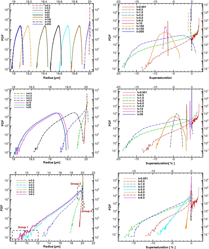
Figure 4. Comparison of the size distribution and the supersaturation pdf for different microphysical coupling constants  or K. The rows correspond to the three rows of table 2, i.e. strongly homogeneous mixing (top row), intermediate mixing (middle row) and strongly inhomogeneous mixing (bottom row). The lower left panel identifies three droplet groups corresponding to the strongly skewed left tail, the mean and the right tail of the diameter pdf. Times in all legends are given in seconds.
Download figure:
Standard imageThe size distributions in figure 4 suggest that significant changes in the shape of the distribution occur early in the mixing process, after which the shape becomes 'frozen in'. We investigate this early development by plotting the size pdfs in terms of δr2, as shown in figure 5, recalling that in r2-coordinates the size distribution maintains a constant shape during uniform condensation or evaporation. The size distributions are plotted for 0.2, 0.4, 0.6, 1.0, 2.0 and 4.0 times the large-eddy time TL (=2.5 s), and it is immediately seen that essentially all the change in the pdf shape occurs for t ⩽ TL. The response of droplets during this transient period of mixing therefore dominates the final shape of the size distribution. This provides a relatively simple explanation for the distinctive shapes resulting from strongly homogeneous and inhomogeneous mixing: during homogeneous mixing the negative supersaturation tail collapses within time TL and the size distribution therefore does not have sufficient time to respond significantly, whereas during inhomogeneous mixing the droplets respond rapidly to the negatively skewed supersaturation pdf and then maintain the resulting shape as the vapor field is thoroughly mixed.

Figure 5. Distributions of square-radius fluctuations δr2 for the three Damköhler numbers studied (upper left: homogeneous, upper right: intermediate, lower: inhomogeneous). Distributions are shown for the following times: 0.2, 0.4. 0.6, 1.0, 2.0 and 4.0 times TL. The corresponding times in the legends are given in seconds.
Download figure:
Standard imageTo understand further the appearance of the negative-exponential tail in the droplet size distribution, we identify three droplet groups, as shown in the lower left panel of figure 4. The groups are chosen from the left tail, center and right tail of a size distribution near the final stages of mixing. There are 3000 droplets in each of the groups, taken from among the total 1.1 million droplets. The positions of these droplets are displayed in figure 6 for times t = 0 and t = 0.2TL, with droplets in groups 1, 2 and 3 being dark blue, light blue and green, respectively. As might have been expected, droplets from group 3 lie mostly away from the interface, within the 'core' of the unmixed cloud, while droplets from groups 1 and 2 are mostly positioned near the clear air–cloud interface. The right panel of figure 6 clearly shows that droplets in group 1, those that experience the most extreme evaporation, tend to lie at the very edge of eddies that are ejected from the initial slab cloud into the clear air during early stages of the mixing process.
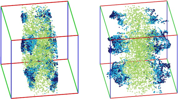
Figure 6. Illustration of the three droplet groups (identified in the lower left panel of figure 4) during the entrainment and mixing process. The left panel shows the positions of all 9000 droplets at the beginning of the mixing process and the right panel illustrates the positions after 0.2TL. Droplets in groups 1, 2 and 3 are shown in dark blue, light blue and light green, respectively.
Download figure:
Standard imageThe Lagrangian behavior of individual droplets from each group is illustrated in figures 7 and 8. Five droplets are selected from each group defined in figure 4 and this is further extended to the other two simulations (droplets similarly sampled from the left tail, center and right tail of each distribution). In figure 7, each row displays radii versus time for a particular value of  , homogeneous mixing for the top row and inhomogeneous mixing for the bottom row. Each column corresponds to a particle group, with group 1 on the left, group 2 in the center, and group 3 on the right. Figure 8 shows supersaturation sampled by the individual droplets versus time, with panels similarly arranged as in figure 7. In all radius versus time plots the phase relaxation is apparent, and as expected, the strongly inhomogeneous mixing scenario shows the most rapid response of droplet size. In that case (bottom row), full relaxation is reached by t ≈ TL, with a nearly linear in time decrease of the droplet radius. The final radius is lowest for group 1 and highest for group 3, as can be understood from the corresponding supersaturation evolution plots, which show a progressively shallower minimum from group 1 to group 3 (figure 8). The supersaturation histories for all scenarios and particle groups are qualitatively similar, with a rapid decrease followed by a somewhat slower, asymptotic increase towards S = 0. The main dip occurs within t ≈ 2TL and is therefore clearly associated with the transient mixing event during the first large-eddy turnover times.

Figure 7. Comparison of the droplet sizes of five particles from each of the three groups depicted in figure 4. The top row is for homogeneous mixing and the bottom row is for inhomogeneous mixing, with groups 1, 2 and 3 in the first, second and third columns, respectively.
Download figure:
Standard image
Figure 8. Comparison of supersaturation of five particles from each of the three groups, as depicted in figure 4. The top row is for homogeneous mixing and the bottom row is for inhomogeneous mixing, with groups 1, 2 and 3 in the first, second and third columns, respectively.
Download figure:
Standard image5. Discussion and summary
The most intriguing regime in this study is that corresponding to strongly inhomogeneous mixing. As we have seen in the last sections, the droplet size distribution then exhibits a pronounced exponential tail. In the following, we give a short explanation of how the left tail of the pdf of r2 follows as a consequence of the pdf of the supersaturation S along the droplet tracks. Equation (5) can be rewritten as

and we then obtain the general solution

This requires a knowledge of the full time history of the supersaturation along the droplet track from the beginning of the mixing to time t. The solution can be simplified to

if the supersaturation S is roughly constant with an average  along the droplet trajectories for a certain time lag starting at
  . Figure 6 (bottom row) shows that this indeed seems to be the case for all three groups between t ≲ 1 and approximately 2.5 s, the latter of which is TL. Thus we take
  . The pdfs of the radius square and supersaturation can be related by the following expression:

The substitution rule for the delta distribution states that

where the prime denotes the derivative of r2 with respect to S taken in (18) at the value  at which
  . This gives
  and
and  . For simplicity, we substitute, furthermore,
  by
by  that we have determined for figure 5 and thus

Supposing that to a good approximation an exponential tail of the supersaturation pdf is established, then for S < 0 we can set

The parameter α will be a function of t and K. For the strongly inhomogeneous mixing regime, the tail of the supersaturation pdf can be matched with α = 0.02, 0.023 and 0.018 for times t = 1, 1.5 and 2 s. Figure 9 demonstrates that the supersaturation pdf with the exponential tail indeed results in a size distribution with a shape that can be matched reasonably well to that prescribed by (22).
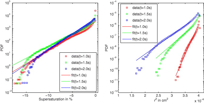
Figure 9. The relation between the supersaturation pdf (left) and the size distribution (right) for the strongly inhomogeneous mixing case. The tails of the supersaturation have been fitted to an exponential with a decay rate α for t = 1, 1.5 and 2 s. The resulting size distributions (the same series of data as in the bottom panel of figure 3, but not rescaled) have been matched with the resulting function on the right-hand side of equation (22).
Download figure:
Standard imageIt remains to be shown why the entrainment process generates exponential tails of the supersaturation pdf. As was seen in figure 4 (right panels), however, its appearance during the transient mixing for t ≲ TL is largely independent of details of the particle response. We draw attention, however, to work done in the context of the so-called Kraichnan model, a passive scalar advection model in a synthetic turbulent flow without time correlations [24] (see [2, 25] for comprehensive reviews). For both spatially rough and smooth advecting flows, it can be shown within this model that exponential tails of the passive scalar evolve. Numerical and experimental studies on Navier–Stokes turbulence can give rise to super-Gaussian or exponential tails as well as to sub-Gaussian tails as discussed in [26]. This difference might be attributed to the finite-time correlations that every real turbulent flow obeys, a point that is still open.
The idealized numerical experiments presented here aimed at exploring extreme cases of mixing and entrainment at the edge of a cloud within a simplified numerical model that disentangles mixing dynamics from the strong temperature feedback via the latent heat release as would be present during the evolution in a cloud. The regimes of strongly homogeneous and inhomogeneous mixing were established here by a manipulation of the droplet response to local super- or subsaturation which is established by a variation of the constant K (or  ) in growth equation (6) for the droplet radius. The strongly inhomogeneous mixing case is characterized by pronounced exponential tails of the pdfs of supersaturation and radius which can be quantitatively related to each other.
As we stated at the beginning of this work, our present study should be considered only as a first step of a longer-term analysis on the complex subject of turbulent mixing in clouds. There is no doubt that it remains to be seen which aspects will be observable when the feedback of the temperature field is included and the numerical experiments are scaled up to larger Reynolds numbers and box sizes which automatically lead to larger Damköhler numbers DaL (e.g. fully resolved cloud volumes of the order of 10 m3). Studies that incorporate the active role of temperature on the flow and the latent heat release in the mixing dynamics are currently under way and will be reported in the near future. However, the present analysis already provides what in our view are interesting implications for models in which groups of 105–106 individual cloud droplets are represented by one quasi-particle, commonly referred to as a super droplet [21, 27]. In those models that are usually coupled to LES the present studies can provide new strategies to model the fluctuations of S on the subgrid scales. Regardless of the mode of implementation, ultimately it will be important to couple the effects of local mixing and dilution, such as those considered here, with the fluctuations in humidity that result from larger-scale motions within the cloud. Recent efforts to perform detailed microphysical calculations for ensembles of Lagrangian parcel trajectories (e.g., [28, 29]) either neglect mixing between parcels or represent the parcel-scale mixing in simple ways that do not fully capture the Damköhler-number dependence. Similar statements could be made regarding recent developments on stochastic condensation theory (e.g. [30, 31]). These approaches give very important insight into the crucial role of large-scale mixing and dynamics in the evolution of droplet size distributions, and it remains to be seen how an accurate representation of the microphysical response to entrainment and dilution will alter the emerging picture.
Acknowledgments
The authors are grateful to Alan Kerstein, Steven Krueger, Alexander Kostinski and Holger Siebert for helpful discussions. The authors acknowledge support from the Deutsche Forschungsgemeinschaft (DFG) within the Research Focus Program Metström (SPP 1276). JS acknowledges additional support from the Heisenberg Program under grant no. SCHU 1410/5-1. Furthermore, support from COST Action MP0806 is kindly acknowledged. The numerical simulations have been carried out at the Jülich Supercomputing Centre (Germany) on the computer cluster JUROPA under grant no. HIL03. RAS acknowledges support from the National Science Foundation under grant no. AGS1026123.