

Abstract
We have designed and built a passively shielded, cryogen-free 3 T 160 mm bore bismuth strontium calcium copper oxide HTS magnet with shielded gradient coils suitable for use in small animal imaging applications. The magnet is cooled to approximately 16 K using a two-stage cryocooler and is operated at 200 A. The magnet has been passively shimmed so as to achieve ±10 parts per million (ppm) homogeneity over a 60 mm diameter imaging volume. We have demonstrated that B0 temporal stability is fit-for-purpose despite the magnet operating in the driven mode. The system has produced good quality spin-echo and gradient echo images. This compact HTS-MRI system is emerging as a true alternative to conventional low temperature superconductor based cryogen-free MRI systems, with much more efficient cryogenics since it operates entirely from a single phase alternating current electrical supply.
Export citation and abstract BibTeX RIS
1. Introduction
There are a growing number of groups reporting MRI imaging using HTS magnets, for example at 1.5 T using a BSCCO based head imaging magnet [1] and at 3 T using a REBCO based magnet [2]. In previous papers we have reported on the design, construction and overall performance of a cryogen-free 1.5 T MRI system constructed from YBCO conductor [3, 4], suitable for orthopaedic applications.
This magnet utilised 4.8 km of conductor wound into 16 double pancake coils. It was cooled to approximately 20 K using a Cryomech PT810 pulse tube cryocooler and run at 130 A in the driven mode (i.e. with a permanently attached, high stability power supply). The magnet had a 240 mm warm bore and an imaging volume with <10 ppm variation over a 120 mm sphere. We investigated the use of unshielded gradient coils with this system, and concluded that, whilst features of the magnet enabled their use, the specific implementation of the conduction cooling system in this magnet led to prohibitively strong coupling between one of the gradient channels and the cooling bus, restricting the system to use with spin-echo imaging sequences only.
Following on from the 1.5 T YBCO system, we were interested in exploring smaller bore, higher field magnets utilising a more efficient cryocooler. An emerging application for cryogen-free MRI magnets is in pre-clinical MRI. Such systems offer pre-clinical users substantial convenience over liquid helium bath cooled low temperature superconductor (LTS) magnets. In particular, laboratory spaces do not require helium quench ducting for their magnets, nor do the magnets require regular cryogen top-ups. Whereas most cryogen-free pre-clinical systems are based around a magnet wound from the LTS NbTi, we have investigated the performance afforded by an HTS cryogen-free system. The magnet is designed to operate at 20 K cooled by a two-stage cryocooler with a helium compressor that only requires a single electrical phase to operate. Combining the magnet with a single electrical phase, air cooled, high stability power supply mean that the entire system may be operated from standard single phase AC power outlets. In order to realise the lowest possible cost HTS magnet implementation, we designed the magnet to use BSCCO conductor. At the time of writing, BSCCO conductor is more cost effective than YBCO conductor [5].
A common specification for cryogen-free pre-clinical MRI systems utilises an actively shielded 3 T magnet with a 160 mm bore and a 60 mm diameter spherical volume [6]. Typically such a system uses a persistent mode magnet wound from NbTi. We have designed our HTS system with identical specifications, but as a passively shielded, driven-mode system (i.e. using a power supply to drive the magnet at all times). Passive shielding small magnets has a number of advantages over actively shielded magnets. It reduces fringe field for a similar sized actively shielded magnet, whilst utilising less superconductor. The magnetisation of the yoke adds an additional magnetic field to that of the coils, improving magnet efficiency. Finally, the substantial mass of the yoke acts as a mass damper for reducing cryocooler vibrations coupling into the magnet coils which may affect the temporal stability of the magnetic field.
2. Design of magnet
2.1. Magnetic design
Magnet optimisation for MRI has been studied extensively in the literature [7], in particular when the magnet has no nonlinear magnetic components. The introduction of a steel yoke complicates the optimisation as calculation of the nonlinear contribution to the magnetic field from the yoke requires a finite element model (FEM). In this instance, the yoke acts as the cryostat in addition to providing the return path for the magnetic flux, hence shielding the magnet. A two layer yoke was chosen to enhance shielding performance whilst reducing weight gain. We typically wind HTS magnets from a number of double pancake coils, since this winding technique is readily compatible with the tape-based BSCCO conductor chosen for this magnet.
We have taken a hybrid approach to designing the uniform magnetic field for this magnet in light of the yoke. This method uses Cobham's Opera finite element software for field calculation and MATLAB for optimisation. For reference, Cobham's Opera finite element software is used for all finite element calculations in this report.
A linear programming method is used to calculate the initial positions of the pancake coils [8]. A 2D FEM is then created with a steel yoke around the coils, where the yoke is designed so as to achieve the desired stray field performance. Using a nonlinear optimisation method, for example Nelder–Mead [9], the coil sizes are iteratively modified inside the FEM until the desired field strength and homogeneity is achieved. The final operation is to create a 3D FEM magnetic model of the magnet taking into account any features that penetrate the yoke or change its shape from the simple 2D representation. As the 3D model is very slow to solve, the final coil positions are calculated by optimising a 2D model to generate the equal and opposite field harmonics found in the 3D model. The final magnet design is shown in figure 1 and specified in table 1.
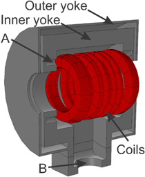
Figure 1. Cross section through the magnet yoke assembly. The coils are shown as red. Note that the yoke has two layers, an outer 'shield' and an inner part that also acts as the cryostat. Label A shows the feature in the yoke designed to accommodate the axial suspension elements of the coil pack. Label B shows the penetration into the yoke for the cryocooler.
Download figure:
Standard image High-resolution imageTable 1. Summary of key magnet specifications.
| Design parameter | Value (units) |
|---|---|
| Design field | 3.04 T |
| Operating current | 200 A |
| Conductor | AMSC BSCCO |
| Current density | 154 A mm−2 |
| Number of pancakes | 18 |
| Total wire length | 3.6 km |
| Inductance | 3.0 H |
| Peak field on coils | 4.14 T |
| Peak hoop stress | 60.5 MPa |
| Peak axial stress | 1.1 MPa |
| Magnet outer diameter | 530 mm |
| Magnet inner diameter | 160 mm |
| Magnet length | 540 mm |
| Imaging DSV | 60 mm |
As can be seen in table 2 this method is not perfect and there are some small residual terms in the low order axial spherical harmonic terms. As may be expected, there is some x and other low order contamination resulting from the feature required for the cryocooler penetration. These terms are easily correctable using passive shimming, and were ultimately found to be much smaller than terms arising during construction.
Table 2. Residual spherical harmonic terms in ppm as measured on the surface of a 60 mm sphere relative to 3 T. In this nomenclature, A3,1 is the cosine component of the 3rd degree, 1st order spherical harmonic.
| Harmonic (on 60 mm DSV) | Value (ppm relative to 3 T) |
|---|---|
| A1, 1 | 41 ppm |
| A2, 2 | −4 ppm |
| A3, 1 | −2 ppm |
| A2, 0 | −2 ppm |
| A4, 0 | −7 ppm |
| A6, 0 | −1 ppm |
| Others | <0.1 ppm |
The fringe field is designed to be very compact, as can be seen in figure 2. The overall weight of the magnet and coil packs is 650 kg. This weight is largely due to the mass of the yoke required to substantially self-shield the magnet.
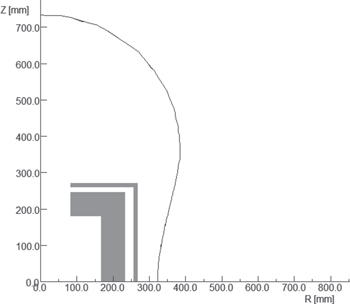
Figure 2. Fringe field of the 3 T MRI magnet. The grey elements are one quarter of the axisymmetric yoke assembly.
Download figure:
Standard image High-resolution imageWe wound the magnet from AMSC BSCCO-2223 conductor. This is a conductor that was manufactured in the early 2000s by AMSC and discontinued, but that we occasionally use for prototyping magnets. For this magnet, we used the high-strength, stainless steel laminated version of the conductor which was supplied wrapped in a paper insulation. The conductor was specified as having a critical stress tolerance of approximately 300 MPa [10], well below the 60.5 MPa hoop stress expected from the magnetic design. The approximate wire dimensions are 4.1 × 0.32 mm with 55 BSCCO filaments embedded in a silver matrix [10]. The average Ic in self-field and at 77 K is >145 A, with an n-value of 16–20 [10]. We verified critical current performance of the conductor using our in-house wire characterisation tool [11] to measure Jc(B, θ, T) data for this conductor. The data at 25 K and at 4 T are shown in figure 3.
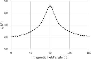
Figure 3. Field angle dependence of critical current for AMSC BSCCO conductor as measured at 25 K and 4 T.
Download figure:
Standard image High-resolution imageBy calculating B and θ at all points in the coils in the 2D FEM, we were able to calculate the local Ic of the coils at all points in the magnet following the methods of [3, 12]. We have chosen to operate the magnet at no greater than 75% of Ic to ensure the magnet will always be operated far from Ic but still retain good conductor utilisation. To fulfil this requirement, we have calculated that the magnet must be run no higher than 25 K.
2.2. Thermal and mechanical design
One of the design aims for this magnet was to utilise the high temperature operation of the magnet to allow use of a cryocooler that only requires a single electrical phase helium compressor. We chose the Oxford Cryosystems LTD Coolstar 6/30 two-stage Gifford–McMahon style cooler, the capacity curve of which is shown in figure 4.

Figure 4. Oxford Cryosystems Coolstar 6/30 cryocooler capacity curve. Figure adapted from Oxford Cryosystems Coolstar brochure.
Download figure:
Standard image High-resolution imageSince the coils shown in figure 1 are located inside a yoke, displacement of the coil pack from the central position causes the coil pack to experience significant body forces. The suspension elements for the magnet must therefore not only minimise the heat leak into the magnet, but also resist the body forces. Since there are no coils connected in a negative sense, all coils in the coil pack experience a compressive axial force. The coils are therefore simply arranged in a stack with appropriately sized spacers between coils where required as shown in figure 5. The coil pack is finally bolted together with a series of M5 stainless steel threaded rods to maintain the concentricity and alignment of the coil pack assembly.

Figure 5. Schematic representation of major coil pack elements.
Download figure:
Standard image High-resolution imageWe designed separate suspension elements to resist forces in the radial (x/y) and axial (z) directions respectively. The coil pack is positioned axially using tubular G10 struts. The coil pack is positioned radially using G10 stands. The position of these two elements can be seen in figure 5. The strength of these structural elements was validated using FEM in light of the force gradients calculated in table 3.
Table 3. Body forces acting on the coil pack assembly upon displacement of the coil pack from the geometric centre of the yoke.
| Coil displacement direction | Force gradient strength (N mm−1) |
|---|---|
| +x | 500 |
| −x | 600 |
| ±y | 600 |
| ±z | 3200 |
The thermal performance of the magnet was calculated by creating a FEM model of the magnet. We chose to eliminate the usual isothermal radiation shield from the magnet, since the Coolstar 6/30 can extract several Watts of heat at 20 K. In this situation, FEM is essential since the high heat flow through the coil pack can lead to unexpected hot spots. The thermal model sets the edges of the structural elements at room temperature (293 K), and the cryocooler attachment point, as shown in figure 5, to 20 K. Other external surfaces that are neither connected to cryocooler, nor at room temperature, are subjected to a radiation load of 2.2 Wm−2, which we have found to be typical for well-installed multi-layer insulation. Interfaces between elements in the coil pack are modelled with a thermal conductivity of 10−3 Wm−1 K−1, which is conservatively modelled as less conductive than greased joints [13]. Nonlinear thermal conductivity for the constituent materials is modelled utilising data from [13]. The temperature distribution over the complete cold assembly is shown in figure 6.

Figure 6. Temperature distribution across cold assembly under expected operating conditions.
Download figure:
Standard image High-resolution imageThe model predicts the cryocooler needs to extract 4 W of heat at 20 K to maintain the coil temperature at 24 K. The temperature variation across the superconducting coils themselves is shown in figure 7.
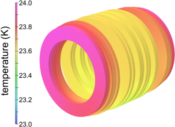
Figure 7. Temperature distribution across coils under expected operating conditions.
Download figure:
Standard image High-resolution imageTypically current is injected into the coil pack via a set of copper current leads from the external environment to the first stage of the cryocooler, then via a set of HTS current leads from the first stage to the second stage, then via HTS leads to the coils. For optimised copper current leads [13], when operating at 200 A, 16.4 W is expected on the first stage of the cryocooler. In this application, there are no further sources of heat loading on the first stage of the cryocooler. Therefore, with 4 W heat extraction on the 2nd stage and 16 W on the 1st stage, the capacity curve for the Oxford Cryosystems cooler indicates that the 2nd stage will operate at 14 K and the 1st stage at approximately 45 K. Using the 4 K difference in temperature calculated between the cryocooler (20 K) and the maximum coil pack temperature in figure 7 (25 K), it is anticipated that the temperature of the coil pack will be approximately 18 K giving 7 K temperature margin between the desired 75% Ic limit and the expected operating temperature.
2.3. Optimisation of thermal bus to minimise gradient interaction
Typically gradient coils use an active shield to minimise the coupling between the magnet and gradient coil systems. However, eliminating the active shield results in very efficient, compact gradient coils. When unshielded gradient coils are pulsed, the resulting transient magnetic field establishes eddy currents in any electrically conductive surfaces near the gradient coils. These eddy currents in turn create an undesirable time-dependent perturbation to the magnetic field, B0, in which MRI is performed. Typically, superconducting magnets use an isothermal radiation shield constructed from a thermally conductive material (e.g. aluminium) to minimise the radiative component of heat load onto the magnet coils. The isothermal radiation shield is often the major source of eddy currents in a superconducting magnet. Historically, the perturbation to B0 arising from eddy currents established in the thermal shield has been unacceptably large for MRI, leading to the design of shielded gradient coils [14] which minimise the exposure of the thermal shield to transient gradient magnetic fields.
In our previous work [3, 4] and here, we have demonstrated that we can eliminate the isothermal radiation shield from the magnet. For such magnets, a common source of eddy currents is eliminated. We have therefore re-investigated the possibility of using unshielded gradient coils for these magnets. Our previous success in using unshielded gradient coils appeared to be limited by a strong coupling between one of the gradient coils and the cooling bus of the magnet [15]. Whilst we have decided to manufacture this system with a set of shielded gradient coils, we also sought to minimise the electromagnetic interaction between the magnet and the gradient systems. We will investigate operation of unshielded coils with this system at a later stage.
Using the primary windings of the shielded gradient set design, we calculated by finite element methods the eddy currents formed in the magnet cooling bus resulting from steady state application of a 100 A, 100 Hz sine wave. Using this method, average heat dissipated in the cooling plates and the magnetic field induced over the imaging volume was calculated for each of the x, y and z gradients with the slitting scheme shown in figure 8.
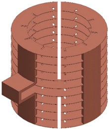
Figure 8. Schematic representation of slitting performed on the thermal bus. There are a combination of partial slits on the internal diameter, and complete slits in two radial locations. The complete slits do not go through all cooling plates to ensure an unbroken thermal path back to the cryocooler for each plate section.
Download figure:
Standard image High-resolution imageThe significant time-averaged spherical harmonics of the Bz component of magnetic field arising from 100 Hz excitation of each of the gradient channels are shown in table 4. In particular there is little difference between the coupling of the x and y channels to the cooling bus, indicating the mechanism that caused the coupling in our earlier work has been eliminated in this design.
Table 4. Heat load and average spherical harmonics induced from application of a steady state 100 Hz, 100 A gradient waveform for each of the X, Y and Z gradients. In this nomenclature, A3,1 is the cosine component of the 3rd degree, 1st order spherical harmonic.
| X gradient | Y gradient | Z gradient |
|---|---|---|
| 0.83 W heat load | 0.78 W heat load | 1.48 W heat load |
| A0, 0 = 28 ppm | A0, 0 = −15 ppm | A0, 0 = −1 ppm |
| A1, 1 = 93 ppm | A1, 1 = −8 ppm | A1, 0 = −115 ppm |
| B1, 1 = −7 ppm | B1, 1 = −82 ppm | A2, 1 = −1 ppm |
| A2, 0 = −6 ppm | A2, 0 = −4 ppm | B2, 1 = −1 ppm |
| B2, 2 = 2 ppm | B2, 2 = −1 ppm | B2, 2 = −1 ppm |
| A3, 1 = −3 ppm | A3, 1 = 3 ppm | A3, 0 = 7ppm |
2.4. Magnet protection
We have designed the magnet to have basic active quench protection. This protection serves two purposes. The first is to protect the magnet in the likely case of power or cooling system failure. The second in the much less likely event of spontaneous quench. In both instances, the method of protection is the same, namely the power supply is disconnected from the magnet using an electrical breaker, and the magnet current run down through an external 0.5 Ω resistor. Using this system, the magnet energy is halved in 4 s and the external resistor experiences a peak 100 V load upon activation of the breaker. The magnet protection system is engaged in three instances; if there is power failure to the system, if an over temperature event is recorded in the magnet, or finally if an over voltage event is recorded in the magnet. Typically power failure or over temperature triggers of the magnet protection system are indicative of external environmental changes and are responsible for all the magnet protection system trigger events described previously. By contrast detection of over voltage is indicative of an event in the magnet itself. Voltage measurement is performed by calculating the differential voltage between the two symmetric magnet halves of the magnet coil assembly. If a differential voltage larger than 10 mV is measured across the coil assembly, the magnet protection system is activated. In a BSCCO (i.e. low n value) magnet, small differential voltage detection is indicative of a portion of the superconducting coil assembly becoming thermally unstable which can lead to damaging temperature rise should the instability lead to quench [16]. Dissipating the magnet's stored energy into the external resistor effectively limits the temperature rise in the coil and hence prevents degradation to the conductor if detection and activation of the protection system is sufficiently fast.
The efficacy of this technique for cryogen-free BSCCO coils has been systematically established for similar magnets using identical protection methods, where a current decay time of 20 s and a detection voltage of 50 mV was found to be sufficient to protect a magnet with comparable stored energy and current density [17]. This behaviour is expected for a low n value HTS conductor such as BSCCO operating at modest current density, since it has been shown there is usually a long delay between the thermal initiation of quench and damaging temperatures being reached under these circumstances [16]. Our voltage detection system has an actuation time of 200 ms, and with the current decay time set at 4 s by choice of the external resistor, the magnet is likely to be well protected in light of a spontaneous quench event.
3. Magnet construction
The magnet was constructed by HTS magnet manufacturer HTS-110 LTD in 2015. The 18 double pancakes were wound and then encapsulated in an epoxy resin system. The critical current performance of each of the coils was performed in liquid nitrogen to verify performance following manufacture. The coils were integrated into the magnet assembly and finally connected together in series. The completed magnet is shown in figure 9. In addition to the physical magnet, the magnet system incorporated an IECO Oy 200 A ultra-high stability magnet power supply, an Oxford Cryosystems LTD helium compressor and an HTS-110 LTD magnet status monitor.

Figure 9. The completed 3 T magnet as-received upon completion of construction from HTS-110 LTD.
Download figure:
Standard image High-resolution image4. Magnet performance
4.1. Cool down and ramp to field
Upon completion of the magnet, it was cooled down to operating temperature using the Oxford Cryosystems cryocooler. The magnet took approximately 80 h to reach operating temperature. The magnet was then brought to full current using a current controlled power supply. Current was incremented in 10 A steps, waiting for thermal equilibrium at the end of each current step before proceeding to the next. The plot of magnet current against field as measured by a Hall sensor is shown in figure 10, showing the magnet reached the design field of 3 T with 200 A current. The temperature of the magnet is shown in figure 11, with the 2nd stage temperature increasing from 13.5 to 13.9 K following ramp to field. The 1st stage temperature increases from 42 to 55 K following ramp to field. The 2nd stage temperatures and the thermal model shown in figure 6 show good agreement, although the smaller difference in temperature between the modelled and actual coil pack and 2nd stage temperatures indicate that the assumed interface thermal resistance may have been too high. The heat load presented to the 1st stage is higher than modelled, suggesting the simple analytical model for the copper current leads may need further development.

Figure 10. Magnetic field versus current as measured by Hall probe during initial ramp to field of the 3 T MRI magnet.
Download figure:
Standard image High-resolution image
Figure 11. Temperature versus current for the 1st and 2nd stages of the cryocooler and the coil pack assembly. Temperature is plotted as a logarithmic scale to better discriminate between the 2nd stage and coil pack data.
Download figure:
Standard image High-resolution image4.2. Magnet homogeneity and shimming
With the magnet operating satisfactorily at full current, a field map was produced. The magnetic field was measured over the surface of a sphere centred at the geometric centre of the magnet. The sphere was divided into 20 axial planes, upon which measurements were performed at 24 radial points. Measurement was performed using a Hall sensor mounted onto a computer controlled 3-axis positioning stage. Figure 12 shows the magnet undergoing field mapping.
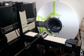
Figure 12. Magnet undergoing plotting using three axis stages. The three stages are attached to the magnet via a jig to improve probe positioning repeatability.
Download figure:
Standard image High-resolution imageAs can be seen in figure 12, we chose to mount the positioning stage on a jig mounted on the magnet to improve measurement repeatability. The result of the field map is shown in figure 13. The initial field homogeneity was similar to the as-built homogeneity of the 1.5 T MRI magnet [4].

Figure 13. As-built magnetic field uniformity for the 3 T MRI magnet. All field measurements in ppm are referenced relative to 3 T.
Download figure:
Standard image High-resolution imageThe gradient coil had been designed with accommodation for passive shim carriers between the primary and secondary coils. Using field plots from the previous 1.5 T MRI work, we determined that if the level of inhomogeneity was similar in this magnet, the magnet could be shimmed using 16 shim carriers with 15 shim positions per carrier. The maximum depth of shim material was set to 2.8 mm, with each piece of shim material measuring 11 × 19 mm. Three different thicknesses of shim were available, and 1006 grade steel was used as the shim material.
Using previously developed passive shimming software [4], following the methods of [18] we corrected gross errors in the homogeneity, and re-measured the homogeneity using a small NMR coil and copper sulphate sample mounted on the same positioning stage as used for the Hall sensor. Signal acquisition was performed using an MR Solutions LTD MRI spectrometer controlled via MATLAB. The homogeneity was greatly improved as shown in figure 14.

Figure 14. Magnetic field uniformity for the 3 T MRI magnet following one shimming operation. All field measurements in ppm are referenced relative to 3 T.
Download figure:
Standard image High-resolution imageTwo more passive shim iterations were subsequently performed. With first order terms nulled out (i.e. using the gradient channels to set these spherical harmonics to zero) as well as Z2, the homogeneity was ∼10 ppm over the 60 mm imaging volume as shown in figure 15. Incorporation of the remainder of the 2nd order shims would improve homogeneity to <2 ppm over the 60 mm imaging volume.
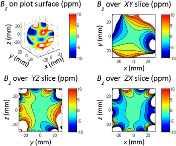
Figure 15. Magnetic field uniformity for the 3 T MRI magnet following completion of shimming. The x, y, z and z2 harmonics have been artificially set to zero in these plots, since they are within the range of the active shims built into the gradient coil assembly, and should hence be zero in the real-world.
Download figure:
Standard image High-resolution imageWe then performed active shimming using the x, y, z and z2 shims. Using standard active shimming techniques, we have achieved a full-width half-maximum NMR line width <1 ppm for a 30 mm diameter spherical sample filled with water, as can be seen in figure 16.

Figure 16. Real-world spectra as measured from a water filled 30 mm diameter sphere. The full-width half-maximum spectral width is 1 ppm relative to 3 T. Frequency is plotted in ppm relative to 3 T.
Download figure:
Standard image High-resolution image4.3. Magnet stability
Upon completion of shimming, we measured the magnet stability. We assess magnet stability over two time frames. The first is the critical time-frame for MRI—that is the time over which acquisition of MRI data usually occurs. Typically this time frames is around a few milliseconds to seconds. Changes in magnetic field over this time appear as changes in phase of the NMR signal, indistinguishable from the desirable change in phase in the NMR signal imparted by the gradient magnetic fields. This spurious change in signal phase leads to ghosting in the MRI image. We undertook the short term measurements using a steady state free precession NMR pulse sequence as seen in figure 17.

Figure 17. Pulse sequence used to measure magnet stability. A series of α RF pulses are played out to give a small flip angle. As for other steady state free precession sequences, a number of warm up pulses are required to ensure the spin system is in a steady state prior to commencing measurements. These are represented by the dashed pulses at the start of the diagram. The black dots represent the samples acquired from each FID.
Download figure:
Standard image High-resolution imageWe acquired the free-induction decay (FID) after each α RF pulse, and calculated the phase angle between the real and imaginary components of the FID for the first few points of the FID. The rate of change in phase is the average change in NMR frequency over the sample points, and hence magnetic field strength. The results of such an experiment are shown in figure 18 with each data point corresponding to one FID. The experiment indicates <16 ppb variation in field over the critical time frame.
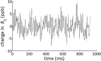
Figure 18. Short term stability of the 3 T MRI magnet as measured using an SSFP sequence. TE = 1 ms. Change in B0 is measured in parts per billion relative to 3 T.
Download figure:
Standard image High-resolution imageAs a driven mode, passively shielded magnet, changes in temperature and small changes in output current of the magnet power supply give rise to changes in the magnetic field of the magnet. The magnet inductance and the 0.5 Ω dump resistor connected in parallel act as a low pass LR filter, with −3 dB point at 26 mHz. Similarly, the large thermal mass of the magnet yoke prevents very fast changes is temperature of the yoke. Such fluctuations in field therefore occur on long time scales, much longer than the critical one second interval. Persistent mode magnets claim very little change in magnetic field strength between measurements since the persistent mode of operation guarantees a change in field of <0.1 ppm h−1. For driven mode magnets, field changes are more random due to the phenomena which contribute to these changes, predominantly temperature. A typical change in field for the 3 T magnet over a 30 h period is shown in figure 19 as measured by calculating change in centre frequency from a series of simple 1-pulse FID experiments. This is a worst case scenario, since the magnet was installed in a non-temperature stabilised room, and the temperature of the yoke was not maintained at a constant level. We anticipate improving the control of ambient temperature and the magnet yoke assembly will result in the long term field drift becoming comparable to the power supply drift specification, namely <1 ppm /30 min.
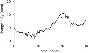
Figure 19. Magnet long term stability as measured from the centre frequency of a series of 1-pulse experiments. Change in field is measured in ppm relative to 3 T.
Download figure:
Standard image High-resolution image5. System construction
Following the completion of the magnet, we designed and constructed an actively shielded three-axis gradient set, which incorporated a B0 and Z2 shim along with provision for passive shimming. The gradient coil had a 160 mm outer diameter and a 100 mm internal diameter. The x, y and z gradient channel strengths were 1.78, 1.89 and 1.42 mT m−1 A−1 respectively, with the gradient amplifier able to produce up to 175 A peak.
We sourced an RF coil and the RF, gradient and shim amplifiers from original equipment manufacturers, and assembled all the magnet and MRI equipment into two  racks. The RF subsystem is shown in figure 20, and uses a simple quarter wave line and crossed diodes to provide decoupling between transmit and receive modes.

Figure 20. Schematic representation of RF subsystem used for the 3 T MRI system. The system uses quarter wavelength lines to achieve decoupling of the low-noise preamplifier during transmit of RF pulses.
Download figure:
Standard image High-resolution imageThe entire RF assembly was enclosed in a Faraday cage formed by the magnet itself and a set of end caps placed over the magnet bore. All the signal and control lines were filtered using in-line capacitors upon entry into the Faraday cage located at the rear of the magnet. The completed system can be seen in figure 21. By comparing noise levels when a 50 Ω load was connected to the input of the low-noise preamplifier, and when the RF coil was connected instead, we ensured the RF receive system had a noise level comparable with near-thermal levels.
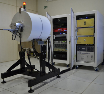
Figure 21. Completed system installed at test facility. In the right hand rack, the magnet power supply and helium compressor for the magnet are housed. In the left hand rack, the amplifiers and spectrometer are housed.
Download figure:
Standard image High-resolution image6. System performance
6.1. MRI imaging
With the magnet operating stably, and with a good level of shim achieved, we performed some MRI images on fruit. We were able to achieve both spin-echo [19] as can be seen in figures 22 and 23 and gradient-echo [19] images as can be seen in figures 24 and 25.
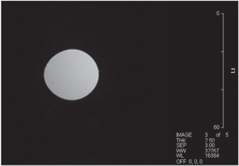
Figure 22. Spin-echo image of 30 mm diameter spherical water sample. Axial image, 100 × 100 mm field of view (FOV). TR = 1500 ms, TE = 300 ms. 2.5 mm slice.
Download figure:
Standard image High-resolution image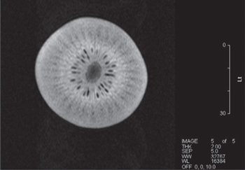
Figure 23. Spin-echo image of kiwi fruit. Axial image, 80 × 80 mm FOV. TR = 3000 ms, TE = 75 ms. 2 mm slice.
Download figure:
Standard image High-resolution image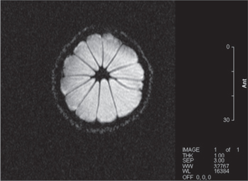
Figure 24. Gradient echo image of lemon. Axial slice, 80 × 80 mm FOV, TR = 500 ms, TE = 9 ms. 1 mm slice.
Download figure:
Standard image High-resolution image
Figure 25. Gradient echo image of 30 mm spherical water sample. Axial slice, FOV = 60 × 60 mm, TR = 500 ms, TE = 9 ms. 1 mm slice.
Download figure:
Standard image High-resolution imageIn previous work, we have only been able to successfully demonstrate the formation of spin-echo images. Refocusing of spins using a 180° radio-frequency pulse as performed in spin-echo imaging is less sensitive to eddy current effects than using a gradient pulse to achieve the same effect. Achievement of gradient echo images without having to use pre-emphasis techniques to accommodate eddy current effects is indicative that interaction between the magnet and gradient set is minimal. This is in part due to the use of a shielded gradient coil, but also due to the optimisation of the cooling manifold to minimise eddy current formation.
We intend to undertake more comprehensive imaging trials to understand if there are any practical limitations of cryogen-free HTS MRI magnets. During these trials we will describe more fully the eddy current coupling between the magnet and the gradient coils.
6.2. Power failure and post-ramp stability
Without the thermal mass of a cryogen bath, cryogen-free magnets will typically exceed operating temperature in the event of power failure. This is due to the magnet warming up once the cryocooler is switched off, causing the magnet to locally exceed Tc, and hence triggering protection circuits. This problem is usually addressed in LTS magnets by adding thermal mass to the system, thereby increasing the length of time the magnet may be held at field before it quenches due to temperature increase. By contrast, driven mode magnets such as our HTS magnet necessarily cannot remain at field during a power outage. Instead, the magnet is allowed to quench into an external dump resistor immediately upon power outage as described previously. During the course of the measurements described in this article, there have been numerous power and water interruptions to the magnet which have caused the magnet energy to be dumped into the external resistor without degradation to the magnet. The magnet is ramped back to full field in 10 min once the magnet is adequately cooled following restoration of power to the magnet.
Once the magnet is back at full field, there is typically a delay before imaging can occur to allow the B0 field to stabilise. The source of B0 instability immediately post-ramp to field in HTS magnets is known to be due to screening currents [20]. Screening currents are induced in the superconductor upon ramp to field, and produce a time-dependent perturbation to the current distribution across the conductor [20]. LTS conductor is multi-filamentary and transposed to avoid such screening current effects; however presently HTS conductor is either mono-filamentary in the case of ReBCO, or multi-filamentary but non-transposed in the case of BSCCO [21]. Accordingly, screening current effects are much larger in HTS conductor than LTS. The effect of the screening current is to change the value and uniformity of B0 with respect to time. Since screening currents decay to a steady state value over time, the decay rate becomes the limiting factor for recommencing imaging, since B0 must be stable for MRI.
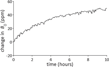
Ramping the magnet directly to 200 A, we measured a 50 ppm change in the magnitude of B0 following completion of the ramp as shown in figure 26. In agreement with other literature [1], we measured an increase in B0 with time, with the exponential decay of the screening currents becoming comparable to the drift in B0 measured in figure 19 after approximately 8 h. Change in uniformity of B0 is also expected due to screening current decay [4]; however, our experience is that the change in B0 uniformity after 8 h is sufficiently stable to allow passive shimming to be reliably performed. If B0 uniformity were changing during the measurements used to calculate passive shim iterations, the passive shimming would not converge to the uniform B0 condition we have demonstrated.
Figure 26. Magnet drift following ramp to field. The initial measurement point occurred approximately 25 min after actual ramp to field to allow initial signal acquisition and active shimming.
Download figure:
Standard image High-resolution image
It is desirable to decrease the settling time between ramp to field and commencement of imaging. The method we intend to investigate more fully is the use of a ramping algorithm. In this method, the final magnet current is overshot slightly, then returned to final current as proposed in [1, 22] which has been demonstrated to substantially reducing magnet settling times in BSCCO magnets.
7. Summary
We have designed and manufactured a 3 T MRI system including an HTS magnet suitable for pre-clinical applications with a 160 mm warm bore and final homogeneity <10 ppm over the 60 mm diameter imaging volume. The magnet was designed with a passive shield resulting in a highly compact magnet both with regards to the size of the magnet itself, and its fringe field. As an HTS magnet, it is highly resistant to spontaneous quench, and to date no such event has been detected during operation of this system. The magnet operates entirely from a single phase AC electrical supply, which is not readily achievable with an equivalent LTS magnet, which typically requires at least a 5 kW three phase electrical supply.
The magnet is sufficiently stable to perform imaging since each NMR acquisition during imaging takes at most a few seconds to perform. However, longer term measurements involving significant averaging will have to take into account B0 drift. This could either be taken into account by changing the RF (i.e. B1) frequency at the start of each NMR acquisition, or by improving the temperature stabilisation of the magnet yoke to reduce drift to the level of the power supply drift.
As an HTS magnet, we have observed changes in B0 consistent with the presence of screening currents; however their presence has neither affected our ability to shim the magnet, nor do they have practical effects on the MRI images we have acquired to data providing adequate settling time is allowed. We are continuing to explore more pulse sequences; however, basic imaging trials using spin-echo and gradient-echo imaging techniques have so far yielded positive results. Our experience with this system to date indicates that there is little practical difference in MRI performance between this HTS magnet based cryogen-free MRI system and LTS based cryogen-free MRI systems.
Acknowledgments
The magnet design and construction work in this article was funded by Kiwinet grant CI001007, and system completion via Ministry of Business, Innovation and Employment grant RTVU1304. The authors would like to thank HTS-110 for peer review and design detailing of the magnet, as well as performing its manufacture. The authors would like to thank Dr Sergei Obruchkov for assistance with imaging and in preparation of the manuscript, Narae Song for performing the passive shimming and Kent Hamilton for developing the Faraday shield design for the system. Finally, the authors would like to thank Fine Instrument Technology for providing data for several of the figures.