
Abstract
In this paper, a Lamb-wave based structural health monitoring for multi-damage localizations in large composite plates is presented. The Lamb waves are generated and received by piezoelectric transducers, which are arranged in array on the composite plate. In the experiments, three composite plates with various laminate stacking sequences and taper designs were prepared. The damages were created on the specimens by impact testing. In each specimen, 24 piezoelectric transducers were utilized and mounted on the specimen surface. This study proposed an algorithm to identify the damage localizations. The transducer layout is classified by 10 subsets. In each subset, the wave propagation paths can be grouped into path groups pivoted by actuators and that by sensors. Based on the damage index, the mean angle line for each path group in a subset can be obtained. By assuming that the mean angle line passes through the actual damage, the damage localization can be achieved if there exist more than two mean angle lines in one subset. In this study, two exclusion rules are proposed to exclude a path group from the damage localization calculations. The damage localization results show that, for a composite plate with multiple damages, their locations can be identified by using multiple subsets. The damage localization results show that the damage location can be accurately predicted for the case that a damage exists in the interior of a subset. The experiment results also show that the Lamb wave characteristics and the localization results are not affected by the thickness variation of the plate, indicating that the proposed algorithm is available for tapered composite plate.
Export citation and abstract BibTeX RIS

Original content from this work may be used under the terms of the Creative Commons Attribution 4.0 license. Any further distribution of this work must maintain attribution to the author(s) and the title of the work, journal citation and DOI.
1. Introduction
The Lamb-wave based structural health monitoring (SHM) has attracted attentions in the recent years as it has been applicable in variety of engineering fields, such as aerospace, civil engineering, etc [1, 2]. Comparing to non-destructive inspection (NDI), the sensors are integrated with or mounted on structures in SHM for real time monitoring. For SHM applications related to the Lamb waves, the waves are generally generated and received by piezoelectric transducers with thin and compact sizes, which are mounted on thin plate structures [3–5]. For metallic structures, the cracks usually initiate at hot spots such as holes or corners. The piezoelectric transducers are mounted near the hot spots [6–9]. The concept of damage index (DI) has been developed to quantify the change between the base signals and current signals. Based on the correlation between DI and crack size, the DI values can be used to evaluate the crack sizes at hot spots [10–15].
The Lamb waves have been also utilized to identify the damage in large plate structures [16]. Unlike the damage size monitoring at hot spots, the damage localization in large plate structures needs more sophisticated algorithms. To increase the detectability, multiple piezoelectric transducers are usually layout as an array, which is called as phase array approach. Huan et al utilized the shear horizontal wave generated by piezoelectric transducer to conduct a high-resolution SHM in a large aluminum plate based on phase array approach [17]. They proposed a linear phase array and the results showed that it can detect a through-thickness hole with a diameter of 2 mm. It can also detect multiple damages. Yu and Tian presented a generic guided wave phased array beamforming method for anisotropic composite laminates [18]. The wave propagation behavior in anisotropic medium was studied in their damage localization model. Senyurek et al proposed a compact phased array for localization of multiple defects in an aluminum plate [19]. In their study, the phased array system was composed of three piezoelectric transducers. They proved that their method does not need to apply high voltages to maintain acceptable signal to noise ratios and can detect multiple defects with high accuracy. Leleux et al utilized the phase array approach and developed a Lamb wave-based SHM technique for large composite plates [20]. The defects they investigated include delaminations and impact damages.
Another approach for damage localization is the delay-and-sum algorithm. This algorithm is based on a fact that a Lamb wave disperses as it propagates through a damage. Wang et al first proposed this approach to detect damages in aluminum plates [21]. This approach has been widely utilized to conduct the damage localization in large aluminum and composite plates [22–26]. In the delay-and-sum algorithm, the damage localization accuracy relies on the group velocities of Lamb waves. For structures with anisotropy or geometric complexity, it is difficult to develop the Lamb wave propagation model, and the application of delay-and-sum algorithm is limited.
For damage localization and damage imaging, the computerized tomography [27, 28], which is inspired by computational tomographic technique used in x-ray imaging, is also a well-developed technique. This technique can offer a damage localization result with high resolution. However, it requires large number of transducers in a relatively small area, i.e. the high transducer density is needed for this technique. The probability-based diagnostic imaging is another approach for presenting damage image by using Lamb waves [29–32]. In this approach, each pixel of the damage imaging corresponds to a calculated probability based on the damage index. The group velocity is no need in the probability calculations so that this approach can be applicable to large complex structures with sparse transducer array.
One of the challenges in some of the previous-mentioned methods in damage localization is that the group velocity analysis model, especially for composite plates for which the group velocity varies with the wave propagation direction. To accurately model the group velocity in composite materials, various approaches have been proposed, including theoretical approaches [33] and experimental measurements [34]. For some methods, the accuracy of the damage localization relies on an accurate model for group velocity as the Lamb wave propagates in composite materials. It restricts the applicability to complex structures.
In this paper, an algorithm for multi-damage localizations in large composite plates by using piezoelectric transducer array is developed and presented. In the present approach, the damage indices and propagation path angles are used in the model for damage localization. There is no need to calculate accurate group velocity so that the proposed algorithm can be applicable to anisotropic composite plates. This study also presents the experiments that contain three composite plate specimens with multiple impact damages. The damage localization results calculated by the algorithm are compared with the real damage locations. This paper is organized as follows. In section 1, the research background and the literature review are presented. The details of the proposed algorithm are given in section 2. In section 3, the experiments, including the specimen preparation, impact testing, piezoelectric transducers and Lamb wave signal acquisitions are presented. The calculations of the algorithm and their comparison to the real damage locations are presented in section 4. The conclusions are given in the last section.
2. Algorithm for damage localization
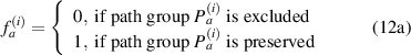
The damage localization algorithm developed in this study is to detect the damage locations in a carbon fiber reinforced plastic (CFRP) plate. It should be mentioned that the ultrasonic wave (Lamb wave) used in this study propagates in the inplane directions of the plate. Thus, the algorithm can identify the inplane location of the damages. The depth of the damage along the thickness direction cannot be identified with this algorithm.
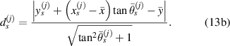
2.1. Damage index (DI) within first arrival window (FAW)
An input signal modulated by a Hanning window is used to excite the actuator. A Lamb wave emitted from the actuator is generated and received by sensor. The received signal contains the electromagnetic interference (EMI), FAW and successive wave packets, as shown in figure 1(a). In figure 1(a),  and
and  denote the signals before and after the damage exists in the specimen, respectively. The time duration
  of the Hanning window is generally identical to that of the FAW, which is formed by the wave packet of fastest Lamb wave mode. The starting time of the FAW can be estimated by calculating the group velocity of the fastest Lamb wave mode. The velocity can be used to determine the distance between the actuator and sensor. The distance must be large enough to avoid the overlap of EMI and FAW. Thus, it is possible to search the actual starting time of FAW between
  and
and  . The time
  is chosen such that
  in order to exclude EMI in the FAW identification. The time
  such that the time interval from
  to
to  comprises FAW. In this time interval, the maximum baseline signal is denoted by
  . Note that
  occurs in the FAW, not in the EMI. This value is used to normalize the signals shown in figure 1. Starting at
  , the jth time stamping is denoted by
  , where
  is the time duration between two adjacent time stampings with a given sampling rate. With the notation
  being the baseline signal at time
  , consider the absolute value of moving average
  of the baseline signal. The value of the moving average at time
  is denoted by
  , which is defined by

Figure 1. Signals received by a piezoelectric transducer: (a) signals before and after the damage; (b) signals within the FAW.
Download figure:
Standard image High-resolution imagewhere  denotes the number of data points in one-quarter period. The relation of
  , excitation frequency
  and the sampling rate
  is given by
The moving average of the signal is calculated by averaging the signal data from  to
to  , where
  denotes the one-quarter period of the sinusoidal excitation signal with frequency
  . During the one-quarter period, there are
  data points to be averaged. The moving average
  is plotted with the time, which is also shown in figure 1(b). In the beginning of the
  curve, the moving average is less than a threshold value. As the FAW comes, the
  curve increases and exceeds the threshold value. By setting this threshold value, the algorithm can identify the starting time of the FAW. In this study, the threshold value is set to be 0.3, i.e. the starting time
  of FAW is to find
  with the lowest
  such that
  . The final time
  of FAW can be estimated by
  . A typical example to search starting time and final time of FAW is shown in figure 1(b).
The baseline signals before and after impact testing are denoted by  and
and  , respectively. Theoretically, a difference between
  and
and  within FAW can be used indicate the existence of a damage. The difference can be evaluated by a damage index DI which is defined by
2.2. Mean angle for a path group
In a subset shown in figure 2, the transducers are arrayed in two rows with horizontal spacing  and vertical spacing
  . There are
  transducers that are assigned as actuators in the first row, while there are
  transducers that are assigned as sensors in the second row. In this study, the number of actuators and sensors is
  . A lamb wave path is a straight line from an actuator to a sensor. A path group
  pivoted at the ith actuator in the subset is formed by four paths emitted from the ith actuator and received by the four sensors, as shown in red lines in figure 2. The jth paths belong to
  are denoted by
  . The propagation angle of path
  is denoted by
  .
.

Figure 2. Illustrations for path groups in one subset.
Download figure:
Standard image High-resolution imageThe path group can be also defined by pivoting at the jth sensor, as the blue dashed line shown in figure 2. A path group  pivoted by the jth sensor in the subset is formed by paths from the four actuators that are received by the jth sensor. The ith paths belong to
  are denoted by
  . The propagation angle of path
  is denoted by
  .
.
It should be noted that  and
and  are actually the same path. They both refer the path from ith actuator to jth sensor. Thus, this path from ith actuator to jth sensor can be simplydenoted by
  . The propagation angle for path
  is denoted by
  . It is obvious that

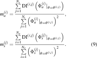
The damage index for path  is denoted by
  .
.
Figure 3 shows the damage indices versus propagation angles for a path group. If the damage is within the subset, the distribution of the damage indices in figure 3(a) should be similar to a Gaussian distribution. The fitting function  of the data DI values for paths in path group
  is given by

Figure 3. Damage indices versus propagation angles for paths belong to path group: (a) DI distribution similar to Gaussian distribution and (b) DI distribution not similar to Gaussian distribution.
Download figure:
Standard image High-resolution image
Similarly, the fitting function  of the data DI values for paths in path group
  is given by

where  ,
,  are constants and
 are the probability density functions of the Gaussian distribution:
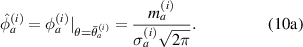
In equation (6),  and
and  are mean angle and standard deviation for path group
  , respectively, while
  and
and  are mean angle and standard deviation for path group
  , respectively. These statistical parameters can be calculated by
where  and
and  are the weighting according to
  :
:
By least square method, the constants  and
and  appeared in equation (8) can be determined by
By using equations (5) and (6), the peak value  of the fitting function for path group
  is
is
Similarly, the peak value  of the fitting function for path group
  is
is
2.3. Damage localization
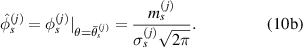
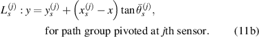
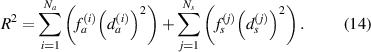
According to the transducer layout, there are eight path groups in one subset, four of which are pivoted by actuators and the rest four of which are by sensors. For the path group  , the damage is assumed to be located on the straight line
  passing through the ith actuator with a slope corresponding to the mean angle
  . Similarly, another straight line
  passing through the jth sensor can also be determined for the path group
  . The straight lines are called the mean angle lines. For locations of ith actuator and jth sensor denoting by
  and
and  , respectively, the mean angle lines can be written by
It should be noted that not every path group can be used for damage localization. Some path groups are excluded from the damage localization calculations. The criterion to exclude a path group will be discussed later. Introduce two parameters  and
and  defined by
Theoretically, by excluding path groups based on the above two exclusion rules, all the preserved mean angle lines pass through the damage location, i.e. these lines are concurrent at this location. However, due to measurement errors or other uncertain reasons, this concurrent does not occur. Suppose the damage location is estimated at a point  . In order to determine this point, consider the distance
  between
  and the mean angle line for path group
  . According to equation (11),
  can be written by
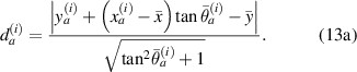
Similarly, the distance  for path group
  is
is
Define a function  by
by
The geometric meaning of  is the summation for the distance square from the point
  to the preserved mean angle lines. Then the solution for
  can be determined by solving the following simultaneous equations:
If all the paths are excluded,  is zero and no damage is detected in this subset.
The maximum  and
and  values for preserved path groups in a subset can be used as an indicator to evaluate the damage size. This maximum value
  can be calculated by

For the case that no path group is preserved,  . The dimensionless distance between the detected location
  and the nearest damage location
  is denoted by
  , which is defined as
where  denotes the horizontal distance between two adjacent transducers, as indicated in figure 2.
2.4. Exclusion rules for path groups
In this study, two exclusion rules for path groups are proposed. The details for the rules are described as follows.
2.4.1. Exclusion rule 1.
The exclusion rule 1 states that a path group is excluded from damage localization calculations if the damage indices for the group do not fit the shape of Gaussian distribution function. For the four paths in one path group, the mean angle line is excluded in the calculation of damage localization if the largest damage index occurs at the first or the fourth path, as shown in figure 3(b). Such damage index distribution usually occurs in the situation that the damage is not located in the range covered by the paths in the path group, or the damage is located on the border of the subset. For this case, the mean angle  (or
(or  ) may have large error in estimating the damage location and should be excluded.
2.4.2. Exclusion rule 2.
It is assumed that the damage index of a path is greater than a certain level if the path passes through the damage. It is expected that the damage indices of the paths in a path group are small if no damage exists. For this case, the path group should be excluded. Thus, the exclusion rule 2 states that a path group is excluded from the damage localization calculations if the damage indices of this path group is less than a specific value. By introducing a threshold damage index  , a path group is excluded from damage localization calculations if

In another case that a damage occurs within a subset, the peak value  (or
(or  ) exceeds
  . However, this path group does not directly interest with the damage. For such case, the damage indices of this path group should be lower than those of other path groups in the subset that are directly affected by the damage. Thus, another reference value
  is introduced and the exclusion rule 2 is modified by


Equation (18) can be considered as a special case of equation (19) by letting  . If
. If  and
and  are both set to be zero, i.e.
  , it means that the exclusion rule 2 is not applied. In the above procedure, the values of
  and
and  are the key parameters that can affect the damage localization results. The threshold damage index
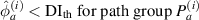
  can be estimated by observing the largest
  and
and  for paths in a subset without damage within it. The determination of
  will be discussed latter.
2.5. Determination of 

As mentioned earlier, the introduction of  is used to exclude the path groups that do not directly interact with the damage. The paths within a subset can be categorized into two types based on whether they hit the damage or not.
  can be defined as the minimum damage index from the paths that hit the damage. The following procedure provides a simple way to estimate
  .
.
The reference damage index  is calculated subset by subset. The transducers in a subset are arrayed such that the numbers of actuators and sensors are
  and
and  , respectively. Therefore, the total number of paths is
  , and there are totally
  damage indices in a subset. In this study,
  and
and  . These damage indices can be ranked according to their values for all paths. Suppose that there exists a damage within a subset. By taking all the damage indices in a subset, they can be sorted in descending order and plotted figure as shown in figure 4. In the descending plot,
  denotes the nth damage index, which means that
  is the largest damage index,
  is the second largest, etc. It is seen that some of the damage indices are significantly higher than the others, indicating that these paths are likely to hit the damage. It is also seen that the
  curve can be roughly divided by two segments with different slopes, and the point where the slope changes can be assigned to determine
  . However, it is not smooth for each of the two segments and the slope change location is not easy to be identified. In order to smooth the curve, introduce
  which is the average value of the damage indices from
  to
to  :
:
Figure 4. Damage index ranking plot in one subset.
Download figure:
Standard image High-resolution image
Figure 4 also shows the  plot, which shows two segments with different slopes. An apex can be identified at the point with slope change. In the
  plot, the coordinate of the nth point can be written as
  . The first point
  and last point
  make a line that makes an angle of
  with the horizontal line. This angle can be calculated by
Define the vector ![${[ {\begin{array}{*{20}{c}} n&{{\text{DI}}_n^{\left( {{\text{ave}}} \right)}} \end{array}}]^{\text{t}}}$](https://content.cld.iop.org/journals/0964-1726/33/4/045028/revision2/smsad3160ieqn159.gif) that started from the origin point
that started from the origin point  to the point
  , where the superscript t denotes the transpose. The rotation of this vector by angle
  counterclockwise about the origin point forms the rotated vector
 ![${[ {\begin{array}{*{20}{c}} {{n^{\left( {{\text{rot}}} \right)}}}&{{\text{DI}}_n^{\left( {{\text{rot}}} \right)}} \end{array}} ]^{\text{t}}}$](https://content.cld.iop.org/journals/0964-1726/33/4/045028/revision2/smsad3160ieqn163.gif) , which can be calculated according to
, which can be calculated according to
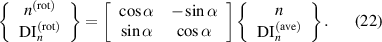
In general, the maximum damage index is approximately equal to 1 and  . With
  , we have
  . It gives that
  is a small angle and


The  plot is shown in figure 4. With the rotation, it is seen that
  . It is also seen that the index
  corresponding to the slope change in
  plot can be obtained by seeking the minimum of the
  plot. Then
  is assigned to be the damage index
  corresponding to this minimum.
3. Specimens and experiments
3.1. Specimen preparation
Three specimens made of CFRP were prepared for the experiments in this study. Each specimen has identical area of 27 in by 21 in (685.8 mm by 533.4 mm). In applications to aircraft engineering, the thickness of the composite plates is generally non-uniform. The tapered thickness is a common seen design. It is well known that the Lamb wave propagation depends on the plate thickness. Thus, three specimens labeled A, B and C are considered, for which three thickness arrangements are presented: no taper (uniform thickness), T1 thickness taper and T2 thickness taper, respectively. The taper design is illustrated in figure 5. According to thickness, the T1 and T2 tapers can be divided into five and nine taper zones, respectively. For tapered specimen, the bottom surface is not flat due to the thickness variation in two adjacent taper zones. The sensors are adhered on the top surface.

Figure 5. Taper design for the composite plate: (a) T1; (b) T2. The unit for dimensions indicated in the figure is in inch and the equivalent values in millimeters are also provided in the parentheses.
Download figure:
Standard image High-resolution imageThe reference stacking sequences is symbolized by  , for which the detail is listed in table 1. The
  laminate has 24 layers, in which a single lamina has a thickness of 0.005 in (0.127 mm). Table 2 lists the details of the stacking sequences of the three specimens. In table 2,
  denotes a stacking sequence by deleting the last n laminas of
  . For specimen A, there is no taper design and the stacking sequence is
  (
( ). It means that the specimen A is stacked by 20 layers. For tapered specimen, the stacking sequence is denoted according to taper zones. For example, the T1 taper is utilized in specimen B and the stacking sequences for taper zones T1–1 to T1–5 are denoted by R-8/R-6/R-4/R-2/R0. All the specimens were fabricated by Aerospace Industrial Development Corporation (Taichung, Taiwan).
Table 1. The reference stacking sequence R0.
| Stacking sequence | Detail |
|---|---|
| R0 | [45, −45, 0, 45, 0, −45, 90, 45, 0, 90, −45, 0]S |
Table 2. Definitions of layer stacking sequences and transducer locations for specimens.
| Specimen | Taper | Stacking sequence | Number of layers |
|---|---|---|---|
| A | No taper | R-4 | 20 |
| B | T1 | R-8/R-6/R-4/R-2/R0 | 16/18/20/22/24 |
| C | T2 | R-8/R-6/R-4/R-2/R0/R-2/R-4/R-6/R-8 | 16/18/20/22/24/22/20/18/16 |
3.2. Impact damage
In the experiment, each specimen was placed on the drop-weight impact testing machine for creating impact damages, as shown in figure 6. The ASTM D7136 test standard was followed. The composite plate was placed on clamping fixture and impacted by an impactor with a mass of 5988 g from a pre-set height. The impact energy can be determined by impactor mass and the height. Each specimen was conducted two experiments. For the first experiment, the impact testing was conducted at three selected locations. In the second experiment, a second impact testing was conducted again at the same locations in each specimen. Two additional locations in each specimen were selected for impact testing in the second experiment. Figure 7 shows the specimens after impact testing. Table 3 lists the details of the impact testing experiments. By using ultrasonic NDI (Olympus OmniScan SX), a damage area was marked for each damage spot. This area can be approximated by an ellipse with horizontal semi-axis  and vertical semi-axis
  . The damage size for each damage in table 3 is denoted by
  .
.

Figure 6. Drop-weight impact testing machine.
Download figure:
Standard image High-resolution image
Figure 7. Impact damage on the CFRP plate: (a) specimen A; (b) specimen B; (c) specimen C.
Download figure:
Standard image High-resolution imageTable 3. Damage locations and sizes measured by NDI for each damage.
| First impact | Second impact | ||||
|---|---|---|---|---|---|
| Damage | Location (mm) | Energy (J) | Damage size (mm) | Energy (J) | Damage size (mm) |
| A-1 | (248, 193) | 20 | 24 × 27 | 30 | 138 × 32 |
| A-2 | (502, 338) | 20 | 18 × 21 | 30 | 171 × 35 |
| A-3 | (184, 490) | 20 | 14 × 29 | 30 | 116 × 36 |
| A-4 | (396, 243) | N.A. | N.A. | 30 | 45 × 33 |
| A-5 | (107, 338) | N.A. | N.A. | 30 | 93 × 21 |
| B-1 | (154, 191) | 20 | 20 × 71 | 25 | 37 × 82 |
| B-2 | (502, 347) | 20 | 24 × 19 | 25 | 42 × 31 |
| B-3 | (184, 474) | 20 | 25 × 55 | 25 | 29 × 77 |
| B-4 | (502, 144) | N.A. | N.A. | 25 | 37 × 17 |
| B-5 | (276, 241) | N.A. | N.A. | 25 | 52 × 25 |
| C-1 | (341, 194) | 20 | 52 × 20 | 20 | 61 × 37 |
| C-2 | (502, 344) | 20 | 21 × 47 | 20 | 45 × 141 |
| C-3 | (184, 489) | 20 | 17 × 30 | 20 | 55 × 35 |
| C-4 | (447, 142) | N.A. | N.A. | 20 | 40 × 27 |
| C-5 | (100, 186) | N.A. | N.A. | 20 | 24 × 67 |
3.3. Piezoelectric transducers
Figure 8 shows the transducer array in one specimen. In each CFRP plate, 24 Smart Layer transducers (Acellent Technologies, Sunnyvale, California) numbered from 1 to 24 are mounted on the top surface. The transducers are arrayed in three rows and eight columns. The distances between two adjacent rows and between two adjacent columns are 63.5 mm (2.5 in) and 152.4 mm (6 in), respectively. The damage locations listed in table 3 are also marked in figure 8 for reference.

Figure 8. Transducer layout and actual damage locations.
Download figure:
Standard image High-resolution imageFor generating Lamb waves, the actuator is excited by a Hamming window signal. The input signal  can be formulated by

where  is the peak voltage of the signal and
  is the Hanning window:
where  is an integer which defines the width of the Hanning window. In this study,
  is used in the experiments. A system composed of Smart Layer transducers, hardware ScanGenie III and a laptop was utilized for signal excitation and acquisition, as shown in figure 9(a). The software SHM Composite (version 2.18.1, Acellent Technologies, Sunnyvale, California) installed in the laptop was utilized to control the hardware and transducers, as shown in figure 9(b). The sampling rate of the receiving signals is
  MHz. Figure 10 shows the dispersion curves for various laminate with different layer sequences. The group velocities shown in figure 10 are calculated with the code GUIGUW (Graphical User Interface for Guided Ultrasonic Waves). The stiffness matrix
  for a lamina with its principal coordinate is given by
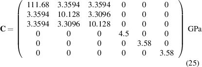

Figure 9. (a) The CFRP plate and the data acquisition system; (b) the software SHM composite.
Download figure:
Standard image High-resolution image
Figure 10. Dispersion curves for various layer stacking sequences with wave propagation directions along (a) path 1–9; (b) path 1–11.
Download figure:
Standard image High-resolution imageThe density and thickness of one lamina is 1750 kg m−3 and 0.005 in (0.127 mm), respectively. By taking the path 1–9 and path 1–11 as examples, the taper zones for the three specimens include  ,
,  and
and  . Note that the plate simulation with GUIGUW must be with uniform thickness. The wave propagates through various thickness along path 1–11 for specimens B and C. For simplification, various thickness conditions are considered for the dispersion curves solved with GUIGUW in figure 10. Also note that the wave propagation characteristics vary with the propagation direction due to the anisotropic behavior of the composite plate. According to the results shown in figure 10, it is seen that the group velocity of the S0 mode approximately keeps constant for frequency less than 300 kHz. For a frequency greater than 300 kHz, the group velocity of S0 mode may be no longer the fastest and the trends of the dispersion curves becomes complex. According to the group velocity shown in figure 10, the shortest time of flight (TOF) between any two transducers is approximately ranged from 30
  to 33
to 33  . The time span of the EMI is approximately equal to that for Hanning window, which is inversely proportional to the frequency
  . For Hanning window with lower frequency, the time span of the EMI could be long and overlap the FAW, causing difficulties in the
  calculations. According to the experimental observations, the time span of EMI for
  kHz is approximately 28
  , which does not overlap the EMI. Thus, three frequencies, 250 kHz, 275 kHz and 300 kHz are utilized to generate the Lamb waves in this study.
The wave propagation in the composite plate was also simulated by finite element software ABAQUS (version 6.14). Due to the limitation of the computation power, partial area with 15 in by 15.5 in (381 mm by 393.7 mm) of the composite plate with transducers 1, 9 and 11 are established. The material properties of the composite are as the same as those used in the dispersion curves shown in figure 10. Unlike the group velocity calculations with GUIGUW, the wave propagation calculations in ABAQUS were conducted with transient analysis. In addition, the three-dimensional geometry in ABAQUS model includes the taper zones with variation of thickness. The C3D8R element in ABAQUS (8-node hexagonal element) is utilized to mesh the composite plate. The transducers are meshed by piezoelectric elements (C3D8E). The input voltage modulated according to equation (24) is applied on the piezoelectric actuator and the output voltage can be monitored as the Lamb waves pass through the sensors. According to a mesh sensitivity test, the element size in the model is approximately equal to 0.8 mm. Figure 11 shows the transient displacement response of the Lamb wave generated by transducer 1 with ABAQUS for specimen C. At the beginning of the wave propagation as shown in figure 11(a), it is seen that the group velocities along vertical and horizontal directions are not the same, indicating the anisotropy of the laminate plates. Figure 11(b) shows the first wave packet, the S0 mode, passing through the transducers 9 and 11 at  . Figure 11(c) shows the displacement contour at
  , revealing that there exist multiple complicated wave packets, which comprise higher-order modes and S0 mode reflected from the boundaries. Thus, it is difficult to identify the modes of the signals received by sensors after
  . Fortunately, these complicated wave packets can be ignored as the FAW only contains the S0 mode, which has the fastest group velocity.

Figure 11. Displacement contours of the wave propagation simulation with ABAQUS for specimen C: (a)  ; (b)
; (b)  ; (c)
; (c)  .
.
Download figure:
Standard image High-resolution imageFor damage localization, some transducers are grouped to belong to one subset. Note that the cover area of a subset cannot be too large. For example, if transducers 1–16 are grouped in one subset, then the wave propagation distance for path 1–9 differs a lot from that for path 1–16. Thus, the comparison of damage indices between these two paths becomes improper. In addition, the signal of a path with long distance may also be weak and become unavailable for damage localization. A subset with too small covering area is also unavailable because of the limited detection area. In this study, ten subsets are assigned, each of which is composed of 8 transducers, as listed in table 4. It should be also noted that the cover area of a subset overlaps that of the adjacent one. This arrangement can increase the detectability of the damage.
Table 4. Subset definitions.
| Subset | Transducer ID assigned to actuator | Transducer ID assigned to sensor |
|---|---|---|
| 1 | 1, 2, 3, 4 | 9, 10, 11, 12 |
| 2 | 2, 3, 4, 5 | 10, 11, 12, 13 |
| 3 | 3, 4, 5, 6 | 11, 12, 13, 14 |
| 4 | 4, 5, 6, 7 | 12, 13, 14, 15 |
| 5 | 5, 6, 7, 8 | 13, 14, 15, 16 |
| 6 | 9, 10, 11, 12 | 17, 18, 19, 20 |
| 7 | 10, 11, 12, 13 | 18, 19, 20, 21 |
| 8 | 11, 12, 13, 14 | 19, 20, 21, 22 |
| 9 | 12, 13, 14, 15 | 20, 21, 22, 23 |
| 10 | 13, 14, 15, 16 | 21, 22, 23, 24 |
4. Results and discussions
4.1. Verification of the FEM results of wave propagation
For the transducer layout shown in figure 8, it should be confirmed that the distance between two transducers of a path is long enough that the starting time of the FAW is longer than the time duration of the EMI. Figure 12 shows the signals for paths 1–9 and 1–11. The excitation frequency is  kHz. For specimen A, no taper design in the layer sequences. For specimens B and C, the taper definitions are shown in figure 5 and table 2. For paths 1–9 and 1–11, the wave propagation paths pass through different thickness region for the three specimens. The FEM results for specimens A, B and C show that the thickness variations do not significantly affect the group velocity of Lamb waves. Figure 12 also shows the measured baseline signals for the two paths of the specimens A, B and C. It is seen that the measured group velocity of the Lamb wave propagating along different paths agree well with the FEM results. For specimen A, the number of layers is 20. For specimen B, the path 1–9 lies on the taper zone T1–2, which has 18 layers. For specimen C, the path 1–9 lies near the border of the taper zones T2–2 and T2–3, which have 18 layers and 20 layers, respectively. The measured results in figure 12 show that no significant difference exists for the starting time of the FAW of path 1–9 in the three specimens. Due to the longer distance, the TOF of the wave for path 1–11 is larger than that for path 1–9. For specimens B and C, the path 1–11 across different taper zones, and similar results for path 1–11 are observed. It should be noted that the group velocity theoretically varies with different plate thickness. Due to the insignificant thickness variation in the tapered plate, the results in figure 12 show that the group velocity is not significantly affected by the thickness variations in the taper designs. The time duration of EMI for
  kHz is
  . The starting time of FAW of path 1–9 for
  kHz is about 40
  . As mentioned in the discussions on figure 11, the FAW contains the S0 mode. For the succeeded wave packets after FAW, they comprise the higher-order modes or the S0 mode reflected from the boundary, and it is difficult to identify the wave modes. For figure 12 shows the wave signals for an excitation frequency of 250 kHz. For the other two driving frequencies, 275 kHz and 300 kHz, the similar results can be obtained.

Figure 12. Comparisons of measured signals and computed signals for  kHz.
kHz.
Download figure:
Standard image High-resolution imageBased on the FEM results and measured data, it is found that the starting time  of FAW is longer than the time duration
  of Hanning window. For the current transducer layout, the FAW is not interfered by the EMI.
4.2. Damage index results
Figure 13 shows the comparisons of baseline signal  and signal
  with damage for paths 6–14 and 11–19. Note that the curves in figure 13 are original, non-normalized signals. The signals are extracted with
  kHz. Note that these signals are original and not normalized. These two paths have vertical path angle, i.e.
  . However, the thickness where the paths located are vary with different specimen. For specimen A, the plate has 20 layers with uniform thickness. For specimen B, the path 6–14 is located in taper zone T1–4 (22 layers), while path 11–19 is in taper zone T1–3 (18 layers). For specimen C, the paths 6–14 and 11–19 are located in taper zones T2–7 (20 layers) and T2–5 (24 layers). Recall that the thickness of each layer is 0.005 in (0.127 mm). The two paths for the three specimens are located in the taper zones ranged from 18 layers to 24 layers. It is seen that the starting time of the FAW (S0 mode) has no significant variations for the two paths in the three specimens. Again, the signals in figure 13 show that the layer sequences for different plates have no significant effect on the group velocity of S0 mode. Recall the damage locations shown in figure 13, there is no damage on the path 6–14 for the three specimens, indicating that the signals with damage are identical to the baseline signal. For path 11–19, there is a damage on this path for specimen A and the signal
  has a difference by comparing
  , as shown in figure 13(a). For path 11–19 in other two specimens, no damage exists on the path and signal
  has no significant difference from
  , as shown in figures 13(b) and (c).

Figure 13. Signals for 300 kHz at second impact for paths 6–14 and 11–19: (a) specimen A; (b) specimen B; (c) specimen C.
Download figure:
Standard image High-resolution imageFigure 14 shows the comparisons of baseline signal  and signal
  with damage for paths 6–16 and 11–21. The signals are extracted with
  kHz. These two paths have the same path angle, i.e.
  . For specimens B and C, the two paths pass through different tapered zones. Similar to the results shown in figure 13, the signals in figure 14 show that the group velocity of S0 mode is nearly independent of the thickness variations in the tapered composite plate. It is also observed that the signal
  has significant change from baseline signal
  if there exists a damage on the path.

Figure 14. Signals for 300 kHz at second impact for paths 6–16 and 11–21: (a) specimen A; (b) specimen B; (c) specimen C.
Download figure:
Standard image High-resolution imageThe dispersion characteristics for Lamb waves propagating through the damage are quite complicated. However, the arrival times of the S0 mode for the baseline signal are equal to that for the signal with damage, as shown in figures 13 and 14. It suggests that the group velocities from the dispersion curves as shown in figure 10 are also valid for waves propagating through damage.
By analyzing the signals from all paths, the damage indices for these paths can be calculated. Figure 15 shows the damage indices for paths in the experiments. By comparing with the damage location shown in figure 8, it is observed large damage indices of the paths that pass through the damages. For example, damages exist on the path 6–16 for the three specimens, and the damage indices for this path in figure 15 are greater than 0.1. It is also observed that the damage indices for path 6–16 after the second impact are greater than those in the first impact.

Download figure:
Standard image High-resolution image
Figure 15. Variations of damage index for various paths, driving frequencies and specimen: (a) damage index for paths in subsets 1–5 at first impact; (b) damage index for paths in subsets 6–10 at second impact; (c) damage index for paths in subsets 1–5 at first impact; (d) damage index for paths in subsets 6–10 at second impact.
Download figure:
Standard image High-resolution image4.3. Reference damage index and threshold damage index
In figure 8, it is observed that no damage exists within subset 3 for the three specimens. The  values are shown in figure 16. In order to determine
  , the values of
  in figure 16 are calculated from the path groups thar are preserved by applying the exclusion rule 1 only, i.e. the exclusion rule 2 is not applied in the calculations of
  . It is seen that the
  values in subset 3 for the first impact experiment are typically lower than 0.005. After the second impact, the
  values for specimen A and specimen B are greater than 0.01 because two damages A-4 and B-5 are located near subset 3. In specimen C, no damage is located near subset 3 after the second impact. Thus, the
  values in subset 3 of specimen C for the second impact are typically unchanged by comparison those for the first impact. According to the
  values in subset 3 after first impact for the three specimens, the
  values less than 0.005 can be considered that no damage exists within a subset. Thus, the threshold value of damage index
  is set as 0.005. For comparisons, two additional
  values,
  and
and  are also considered in this study.

Figure 16.
 for subset 3 with exclusion rule 1.
Download figure:
Standard image High-resolution imageTables 5 and 6 list the reference damage index  and
and  for the subsets in the three specimens. Two sets of
  values are presented here for each case. The first set of
  values determined by applying exclusion rule 1 are presented. By applying equation (19) (the exclusion rule 2) on the first set of
  values and letting
  , the second set of
  values are also presented. For the
  values are zero for some subsets, it means that all the path groups have been excluded by applying the exclusion rules. For a subset that a damage exists within it, the
  values are higher. A typical example is the subset 5 for the three specimens. Large
  values in subset 5 for all cases are observed. For such cases, no further path groups can be excluded by applying the exclusion rule 2.
Table 5.
 and
and  at first impact.
| A 250 kHz | A 275 kHz | A 300 kHz | |||||||

|

|

| |||||||
| Subset |

| Exclusion rule 1 | Exclusion rule 1 + 2 |

| Exclusion rule 1 | Exclusion rule 1 + 2 |

| Exclusion rule 1 | Exclusion rule 1 + 2 |
| 1 | 0.002237 | 0.004892 | 0 | 0.002558 | 0.007833 | 0.007833 | 0.005298 | 0.014592 | 0.014592 |
| 2 | 0.003237 | 0.004768 | 0 | 0.003539 | 0.010662 | 0.010662 | 0.005899 | 0.020309 | 0.020309 |
| 3 | 0.003272 | 0.004438 | 0 | 0.002336 | 0.003549 | 0 | 0.006587 | 0.006875 | 0.006875 |
| 4 | 0.007258 | 0.112085 | 0.112085 | 0.004919 | 0.138972 | 0.138972 | 0.013038 | 0.175116 | 0.175116 |
| 5 | 0.007258 | 0.088022 | 0.088022 | 0.068046 | 0.114532 | 0.114532 | 0.076643 | 0.14311 | 0.14311 |
| 6 | 0.004052 | 0.015721 | 0.015721 | 0.007268 | 0.044187 | 0.044187 | 0.012349 | 0.063501 | 0.063501 |
| 7 | 0.004014 | 0.015391 | 0.015391 | 0.007118 | 0.041041 | 0.041041 | 0.012349 | 0.059177 | 0.059177 |
| 8 | 0.002892 | 0 | 0 | 0.007828 | 0 | 0 | 0.007053 | 0.006482 | 0 |
| 9 | 0.001841 | 0.002423 | 0 | 0.000732 | 0.00296 | 0 | 0.002197 | 0.005899 | 0.005899 |
| 10 | 0.000736 | 0.00274 | 0 | 0.000732 | 0.003306 | 0 | 0.002197 | 0.005494 | 0.005494 |
| B 250 kHz | B 275 kHz | B 300 kHz | |||||||

|

|

| |||||||
| Subset |

| Exclusion rule 1 | Exclusion rule 1 + 2 |

| Exclusion rule 1 | Exclusion rule 1 + 2 |

| Exclusion rule 1 | Exclusion rule 1 + 2 |
| 1 | 0.000371 | 0.00132 | 0 | 0.001005 | 0.001295 | 0 | 0.000974 | 0.002039 | 0 |
| 2 | 0.000403 | 0.001479 | 0 | 0.000709 | 0.001751 | 0 | 0.000974 | 0.001967 | 0 |
| 3 | 0.000276 | 0.00036 | 0 | 0.000477 | 0.000448 | 0 | 0.000508 | 0.001229 | 0 |
| 4 | 0.00912 | 0 | 0 | 0.006574 | 0.000618 | 0 | 0.005945 | 0.001009 | 0 |
| 5 | 0.032622 | 0.128403 | 0.032622 | 0.032964 | 0.141268 | 0.141268 | 0.033568 | 0.228174 | 0.228174 |
| 6 | 0.011476 | 0.069699 | 0.011476 | 0.011613 | 0.078845 | 0.078845 | 0.008179 | 0.088286 | 0.088286 |
| 7 | 0.001945 | 0.001823 | 0 | 0.003243 | 0.003512 | 0 | 0.005377 | 0.004988 | 0 |
| 8 | 0.000789 | 0.001781 | 0 | 0.002673 | 0.003727 | 0 | 0.004968 | 0.006111 | 0.006111 |
| 9 | 0.001114 | 0.000931 | 0 | 0.003243 | 0.005872 | 0.005872 | 0.006263 | 0.011106 | 0.011106 |
| 10 | 0.000771 | 0.002581 | 0 | 0.002958 | 0.005397 | 0.005397 | 0.005984 | 0.01041 | 0.01041 |
| C 250 kHz | C 275 kHz | C 300 kHz | |||||||

|

|

| |||||||
| Subset |

| Exclusion rule 1 | Exclusion rule 1 + 2 |

| Exclusion rule 1 | Exclusion rule 1 + 2 |

| Exclusion rule 1 | Exclusion rule 1 + 2 |
| 1 | 0.000505 | 0.001242 | 0 | 0.000993 | 0.001199 | 0 | 0.000823 | 0.001701 | 0 |
| 2 | 0.000803 | 0.000793 | 0 | 0.001075 | 0.002237 | 0 | 0.001517 | 0.002703 | 0 |
| 3 | 0.000971 | 0.001191 | 0 | 0.001109 | 0.002039 | 0 | 0.001517 | 0.0027 | 0 |
| 4 | 0.030832 | 0 | 0 | 0.043142 | 0 | 0 | 0.045035 | 0 | 0 |
| 5 | 0.071987 | 0.430603 | 0.071987 | 0.088001 | 0.533777 | 0.533777 | 0.090257 | 0.590221 | 0.590221 |
| 6 | 0.001322 | 0.001384 | 0 | 0.002014 | 0.001907 | 0 | 0.003635 | 0.003699 | 0 |
| 7 | 0.003876 | 0.033914 | 0.003876 | 0.01029 | 0.047066 | 0.047066 | 0.016414 | 0.10309 | 0.10309 |
| 8 | 0.006738 | 0.029297 | 0.006738 | 0.01029 | 0.043364 | 0.043364 | 0.024138 | 0.12118 | 0.12118 |
| 9 | 0.005255 | 0.023021 | 0.005255 | 0.008865 | 0.028498 | 0.028498 | 0.009286 | 0.015392 | 0.015392 |
| 10 | 0.001327 | 0.003174 | 0 | 0.004193 | 0.007685 | 0.007685 | 0.006221 | 0.008338 | 0.008338 |
Table 6.
 and
and  at second impact.
| A 250 kHz | A 275 kHz | A 300 kHz | |||||||

|

|

| |||||||
| Subset |

| Exclusion rule 1 | Exclusion rule 1 + 2 |

| Exclusion rule 1 | Exclusion rule 1 + 2 |

| Exclusion rule 1 | Exclusion rule 1 + 2 |
| 1 | 0.003503 | 0 | 0 | 0.005534 | 0.00305 | 0 | 0.007188 | 0.00482 | 0 |
| 2 | 0.003503 | 0.013928 | 0.013928 | 0.002868 | 0.002974 | 0 | 0.003194 | 0.006149 | 0.006149 |
| 3 | 0.005189 | 0.015201 | 0.015201 | 0.002222 | 0.011456 | 0.011456 | 0.005744 | 0.015052 | 0.015052 |
| 4 | 0.014061 | 0.015953 | 0.015953 | 0.0118 | 0.013646 | 0.013646 | 0.01464 | 0.017541 | 0.017541 |
| 5 | 0.074664 | 0.675766 | 0.675766 | 0.064139 | 0.741718 | 0.741718 | 0.063119 | 0.747812 | 0.747812 |
| 6 | 0.038815 | 0.380774 | 0.380774 | 0.044088 | 0.486001 | 0.486001 | 0.044205 | 0.562601 | 0.562601 |
| 7 | 0.038693 | 0.380111 | 0.380111 | 0.029563 | 0.516052 | 0.516052 | 0.026241 | 0.60401 | 0.60401 |
| 8 | 0.038693 | 0.465831 | 0.465831 | 0.029563 | 0.507919 | 0.507919 | 0.026241 | 0.555014 | 0.555014 |
| 9 | 0.029942 | 0.616899 | 0.616899 | 0.020298 | 0.644286 | 0.644286 | 0.026241 | 0.700275 | 0.700275 |
| 10 | 0.010239 | 0.641028 | 0.641028 | 0.017434 | 0.672212 | 0.672212 | 0.02373 | 0.749241 | 0.749241 |
| B 250 kHz | B 275 kHz | B 300 kHz | |||||||

|

|

| |||||||
| Subset |

| Exclusion rule 1 | Exclusion rule 1 + 2 |

| Exclusion rule 1 | Exclusion rule 1 + 2 |

| Exclusion rule 1 | Exclusion rule 1 + 2 |
| 1 | 0.00416 | 0 | 0 | 0.003613 | 0 | 0 | 0.00289 | 0.008651 | 0.008651 |
| 2 | 0.003164 | 0.003121 | 0 | 0.002158 | 0.008646 | 0.008646 | 0.002364 | 0.011631 | 0.011631 |
| 3 | 0.002542 | 0.003082 | 0 | 0.002158 | 0.00879 | 0.00879 | 0.001883 | 0.010951 | 0.010951 |
| 4 | 0.021272 | 0 | 0 | 0.013282 | 0 | 0 | 0.011551 | 0 | 0 |
| 5 | 0.107497 | 0.449442 | 0.449442 | 0.106646 | 0.499151 | 0.499151 | 0.110235 | 0.569612 | 0.569612 |
| 6 | 0.111617 | 0.612702 | 0.612702 | 0.120673 | 0.683718 | 0.683718 | 0.076422 | 0.611747 | 0.611747 |
| 7 | 0.027451 | 0.147941 | 0.147941 | 0.042361 | 0.12822 | 0.12822 | 0.042905 | 0.121631 | 0.121631 |
| 8 | 0.027451 | 0.025581 | 0 | 0.042361 | 0.036622 | 0 | 0.052929 | 0.046805 | 0 |
| 9 | 0.013795 | 0.033626 | 0.033626 | 0.024567 | 0.034819 | 0.034819 | 0.012553 | 0.046012 | 0.046012 |
| 10 | 0.012014 | 0.015485 | 0.015485 | 0.024567 | 0.023241 | 0 | 0.044383 | 0.044586 | 0.044586 |
| C 250 kHz | C 275 kHz | C 300 kHz | |||||||

|

|

| |||||||
| Subset |

| Exclusion rule 1 | Exclusion rule 1 + 2 |

| Exclusion rule 1 | Exclusion rule 1 + 2 |

| Exclusion rule 1 | Exclusion rule 1 + 2 |
| 1 | 0.002228 | 0.002781 | 0 | 0.001444 | 0.001774 | 0 | 0.00132 | 0.002271 | 0 |
| 2 | 0.001737 | 0.002352 | 0 | 0.000752 | 0.001714 | 0 | 0.001371 | 0.002284 | 0 |
| 3 | 0.001001 | 0.00173 | 0 | 0.001703 | 0.001969 | 0 | 0.001482 | 0.002299 | 0 |
| 4 | 0.051323 | 0 | 0 | 0.090943 | 0 | 0 | 0.08858 | 0 | 0 |
| 5 | 0.087734 | 1.041138 | 1.041138 | 0.090943 | 1.17228 | 1.17228 | 0.08858 | 1.175354 | 1.175354 |
| 6 | 0.008287 | 0 | 0 | 0.009084 | 0.002581 | 0 | 0.010456 | 0.003732 | 0 |
| 7 | 0.01583 | 0.144415 | 0.144415 | 0.015484 | 0.188227 | 0.188227 | 0.016415 | 0.264003 | 0.264003 |
| 8 | 0.065414 | 0.132029 | 0.132029 | 0.07341 | 0.182225 | 0.182225 | 0.073041 | 0.268669 | 0.268669 |
| 9 | 0.049657 | 0.214551 | 0.214551 | 0.071631 | 0.222933 | 0.222933 | 0.07708 | 0.250494 | 0.250494 |
| 10 | 0.034132 | 0.297522 | 0.297522 | 0.037361 | 0.327166 | 0.327166 | 0.049269 | 0.363936 | 0.363936 |
4.4. Damage localization results
Figures 17–19 show the damage localization results for specimens A, B and C, respectively. Three different threshold damage indices ( , 0.005 and 0.01) are considered in the calculations. In each specimen, both the actual damage locations and the damage localization locations are marked for comparison. Each specimen was undergone two impact tests. The damage localization results obtained for the first impact and second impact are presented. In general, if a damage is within the transducer layout, it can be detected by one or more subsets. For example, consider damage B-1 shown in figure 18. It can be detected by the paths in subset 6. For the other damages that are within the transducer layout, most of them are identified by the present method. Conversely, damages A-3, A-5, B-3, C-3 and C5 are not within the transducer layout and are difficult to be identified.

Figure 17. Damage localization results for specimen A.
Download figure:
Standard image High-resolution image
Figure 18. Damage localization results for specimen B.
Download figure:
Standard image High-resolution image
Figure 19. Damage localization results for specimen C.
Download figure:
Standard image High-resolution imageTables 7–15 list the damage localization results for each subset of specimens under various driving frequencies and threshold damage indices. If two or more mean angle lines are preserved in a subset, a damage location prediction  is obtained. Then the damage identified by the calculation is assumed to be the nearest actual damage to
  . Also, the dimensionless distance
  between the predicted location and actual location of the damage is also given in tables 7–15. For example, consider the subset 5 in specimen A, the damage localization results of which are listed in table 7. The damage localization location with 250 kHz after the 2nd impact is (504.16, 337.12) in mm. This location remains the same as the threshold damage index ranged from 0 to 0.01. The nearest actual damage is A-2, which is located at (501.65, 337.60) in mm. The distance between the predicted damage location actual damage location is 2.56 mm, resulting a dimensionless distance
  . For subsets that
  , the damage localization results are inaccurate and are marked by 'star'. For the case of
  , some path groups are preserved due to the low threshold value. These path groups have low
  values, indicating that no significant damage signals detected. It results in more subsets are marked by 'star' for
  . By increasing the threshold value, say
  or
or  , the number of the subsets marked by 'star' are significantly reduced. It is concluded that by assigning proper value of
  , the damage localization results are more accurate.
Table 7. Damage localization results for specimen A at 250 kHz.
| 1st impact | 2nd impact | |||||||||||||||
|---|---|---|---|---|---|---|---|---|---|---|---|---|---|---|---|---|

|

|

|

|

|

| |||||||||||
| Subset | Damage identified |

| Damage identified |

| Damage identified |

| Damage identified |

| Damage identified |

| Damage identified |

| ||||
| 1 | A-3 | 0.933 | ||||||||||||||
| 2 | A-3 | 2.122 | ||||||||||||||
| 3 | A-1 | 2.797 | ||||||||||||||
| 4 | A-2 | 0.401 | A-2 | 0.401 | A-2 | 0.401 | ||||||||||
| 5 | A-2 | 0.412 | A-2 | 0.412 | A-2 | 0.412 | A-2 | 0.040 | A-2 | 0.040 | A-2 | 0.040 | ||||
| 6 | A-1 | 0.626 | A-1 | 0.626 | A-1 | 1.122 | A-1 | 0.076 | A-1 | 0.076 | A-1 | 0.076 | ||||
| 7 | A-1 | 0.890 | A-1 | 0.890 | A-1 | 0.983 | A-1 | 0.024 | A-1 | 0.024 | A-1 | 0.024 | ||||
| 8 | A-4 | 0.965 | A-4 | 0.965 | A-4 | 0.965 | ||||||||||
| 9 | A-1 | 3.188 | A-4 | 0.261 | A-4 | 0.261 | A-4 | 0.261 | ||||||||
| 10 | A-2 | 1.382 | ||||||||||||||

Table 8. Damage localization results for specimen A 275 kHz.
| 1st impact | 2nd impact | |||||||||||||||
|---|---|---|---|---|---|---|---|---|---|---|---|---|---|---|---|---|

|

|

|

|

|

| |||||||||||
| Subset | Damage identified |

| Damage identified |

| Damage identified |

| Damage identified |

| Damage identified |

| Damage identified |

| ||||
| 1 | A-3 | 1.514 | A-3 | 0.997 | ||||||||||||
| 2 | ||||||||||||||||
| 3 | A-1 | 2.154 | A-4 | 1.166 | A-4 | 0.556 | ||||||||||
| 4 | ||||||||||||||||
| 5 | A-2 | 0.116 | A-2 | 0.116 | A-2 | 0.116 | ||||||||||
| 6 | A-1 | 0.673 | A-1 | 0.673 | A-1 | 0.183 | A-1 | 0.066 | A-1 | 0.066 | A-1 | 0.066 | ||||
| 7 | A-1 | 0.260 | A-1 | 0.260 | A-1 | 0.260 | A-1 | 0.046 | A-1 | 0.046 | A-1 | 0.046 | ||||
| 8 | A-4 | 0.493 | A-4 | 0.493 | A-4 | 0.493 | ||||||||||
| 9 | A-4 | 0.239 | A-4 | 0.239 | A-4 | 0.239 | ||||||||||
| 10 | A-2 | 2.579 | ||||||||||||||

Table 9. Damage localization results for specimen A 300 kHz.
| 1st impact | 2nd impact | |||||||||||||||||
|---|---|---|---|---|---|---|---|---|---|---|---|---|---|---|---|---|---|---|

|

|

|

|

|

| |||||||||||||
| Subset | Damage identified |

| Damage identified |

| Damage identified |

| Damage identified |

| Damage identified |

| Damage identified |

| ||||||
| 1 | A-3 | 1.417 | A-3 | 1.417 | A-3 | 1.384 | ||||||||||||
| 2 | ||||||||||||||||||
| 3 | A-4 | 1.416 | A-4 | 1.416 | A-4 | 0.744 | ||||||||||||
| 4 | ||||||||||||||||||
| 5 | A-2 | 1.572 | A-2 | 1.572 | A-2 | 1.572 | A-2 | 0.122 | A-2 | 0.122 | A-2 | 0.122 | ||||||
| 6 | A-1 | 0.194 | A-1 | 0.194 | A-1 | 0.194 | A-1 | 0.062 | A-1 | 0.062 | A-1 | 0.062 | ||||||
| 7 | A-1 | 0.166 | A-1 | 0.166 | A-1 | 0.166 | A-1 | 0.041 | A-1 | 0.041 | A-1 | 0.041 | ||||||
| 8 | A-4 | 0.498 | A-4 | 0.498 | A-4 | 0.498 | ||||||||||||
| 9 | A-1 | 2.532 | A-1 | 2.523 | A-4 | 0.215 | A-4 | 0.215 | A-4 | 0.215 | ||||||||
| 10 | A-2 | 2.150 | A-2 | 4.668 | ||||||||||||||

Table 10. Damage localization results for specimen B 250 kHz.
| 1st impact | 2nd impact | |||||||||||||||||
|---|---|---|---|---|---|---|---|---|---|---|---|---|---|---|---|---|---|---|

|

|

|

|

|

| |||||||||||||
| Subset | Damage identified |

| Damage identified |

| Damage identified |

| Damage identified |

| Damage identified |

| Damage identified |

| ||||||
| 1 | B-1 | 1.649 | ||||||||||||||||
| 2 | B-3 | 1.761 | ||||||||||||||||
| 3 | B-5 | 1.425 | ||||||||||||||||
| 4 | ||||||||||||||||||
| 5 | B-2 | 0.091 | B-2 | 0.091 | B-2 | 0.228 | B-2 | 0.109 | B-2 | 0.109 | B-2 | 0.109 | ||||||
| 6 | B-1 | 0.147 | B-1 | 0.147 | B-1 | 0.368 | B-1 | 0.145 | B-1 | 0.145 | B-1 | 0.145 | ||||||
| 7 | B-5 | 0.122 | B-5 | 0.122 | B-5 | 0.122 | ||||||||||||
| 8 | B-1 | 3.403 | ||||||||||||||||
| 9 | ||||||||||||||||||
| 10 | B-2 | 0.454 | B-4 | 0.434 | B-4 | 0.434 | B-4 | 0.434 | ||||||||||

Table 11. Damage localization results for specimen B 275 kHz.
| 1st impact | 2nd impact | |||||||||||||||||
|---|---|---|---|---|---|---|---|---|---|---|---|---|---|---|---|---|---|---|

|

|

|

|

|

| |||||||||||||
| Subset | Damage identified |

| Damage identified |

| Damage identified |

| Damage identified |

| Damage identified |

| Damage identified |

| ||||||
| 1 | B-1 | 1.812 | ||||||||||||||||
| 2 | B-5 | 0.527 | B-5 | 0.527 | ||||||||||||||
| 3 | B-5 | 1.233 | B-5 | 1.233 | ||||||||||||||
| 4 | ||||||||||||||||||
| 5 | B-2 | 0.077 | B-2 | 0.077 | B-2 | 0.193 | B-2 | 0.084 | B-2 | 0.084 | B-2 | 0.084 | ||||||
| 6 | B-1 | 0.108 | B-1 | 0.108 | B-1 | 0.270 | B-1 | 0.219 | B-1 | 0.219 | B-1 | 0.219 | ||||||
| 7 | B-1 | 3.117 | B-5 | 0.169 | B-5 | 0.169 | B-5 | 0.169 | ||||||||||
| 8 | B-1 | 3.303 | ||||||||||||||||
| 9 | B-4 | 1.637 | B-4 | 1.637 | B-4 | 1.637 | ||||||||||||
| 10 | B-2 | 0.924 | ||||||||||||||||

Table 12. Damage localization results for specimen B 300 kHz.
| 1st impact | 2nd impact | |||||||||||||||||
|---|---|---|---|---|---|---|---|---|---|---|---|---|---|---|---|---|---|---|

|

|

|

|

|

| |||||||||||||
| Subset | Damage identified |

| Damage identified |

| Damage identified |

| Damage identified |

| Damage identified |

| Damage identified |

| ||||||
| 1 | B-3 | 1.747 | ||||||||||||||||
| 2 | B-5 | 0.530 | B-5 | 0.530 | ||||||||||||||
| 3 | B-2 | 2.985 | B-5 | 0.731 | B-5 | 1.117 | ||||||||||||
| 4 | ||||||||||||||||||
| 5 | B-2 | 0.121 | B-2 | 0.121 | B-2 | 0.302 | B-2 | 0.086 | B-2 | 0.086 | B-2 | 0.086 | ||||||
| 6 | B-1 | 0.134 | B-1 | 0.134 | B-1 | 0.334 | B-1 | 0.256 | B-1 | 0.256 | B-1 | 0.256 | ||||||
| 7 | B-5 | 0.191 | B-5 | 0.191 | B-5 | 0.191 | ||||||||||||
| 8 | B-1 | 3.329 | B-1 | 3.391 | ||||||||||||||
| 9 | B-4 | 1.192 | B-4 | 1.192 | B-4 | 1.192 | ||||||||||||
| 10 | B-2 | 0.758 | B-2 | 0.758 | ||||||||||||||

Table 13. Damage localization results for specimen C 250 kHz.
| 1st impact | 2nd impact | |||||||||||||||||
|---|---|---|---|---|---|---|---|---|---|---|---|---|---|---|---|---|---|---|

|

|

|

|

|

| |||||||||||||
| Subset | Damage identified |

| Damage identified |

| Damage identified |

| Damage identified |

| Damage identified |

| Damage identified |

| ||||||
| 1 | C-3 | 1.851 | C-1 | 1.710 | ||||||||||||||
| 2 | C-1 | 2.266 | ||||||||||||||||
| 3 | C-1 | 2.611 | ||||||||||||||||
| 4 | ||||||||||||||||||
| 5 | C-2 | 0.325 | C-2 | 0.325 | C-2 | 0.813 | C-2 | 0.098 | C-2 | 0.098 | C-2 | 0.098 | ||||||
| 6 | ||||||||||||||||||
| 7 | C-1 | 0.333 | C-1 | 0.333 | C-1 | 0.832 | C-1 | 0.281 | C-1 | 0.281 | C-1 | 0.281 | ||||||
| 8 | C-1 | 0.038 | C-1 | 0.038 | C-1 | 0.094 | C-1 | 0.401 | C-1 | 0.401 | C-1 | 0.401 | ||||||
| 9 | C-4 | 0.805 | C-4 | 0.805 | C-4 | 0.805 | ||||||||||||
| 10 | C-2 | 0.873 | C-4 | 0.113 | C-4 | 0.113 | C-4 | 0.113 | ||||||||||

Table 14. Damage localization results for specimen C 275 kHz.
| 1st impact | 2nd impact | |||||||||||||||||
|---|---|---|---|---|---|---|---|---|---|---|---|---|---|---|---|---|---|---|

|

|

|

|

|

| |||||||||||||
| Subset | Damage identified |

| Damage identified |

| Damage identified |

| Damage identified |

| Damage identified |

| Damage identified |

| ||||||
| 1 | C-3 | 0.864 | C-3 | 0.781 | ||||||||||||||
| 2 | C-3 | 1.803 | C-3 | 2.098 | ||||||||||||||
| 3 | C-1 | 2.349 | ||||||||||||||||
| 4 | ||||||||||||||||||
| 5 | C-2 | 0.256 | C-2 | 0.256 | C-2 | 0.640 | C-2 | 0.134 | C-2 | 0.134 | C-2 | 0.134 | ||||||
| 6 | ||||||||||||||||||
| 7 | C-1 | 0.356 | C-1 | 0.356 | C-1 | 0.890 | C-1 | 0.305 | C-1 | 0.305 | C-1 | 0.305 | ||||||
| 8 | C-1 | 0.235 | C-1 | 0.235 | C-1 | 0.589 | C-1 | 0.482 | C-1 | 0.482 | C-1 | 0.482 | ||||||
| 9 | C-1 | 0.799 | C-1 | 0.799 | C-1 | 1.996 | C-4 | 0.787 | C-4 | 0.787 | C-4 | 0.787 | ||||||
| 10 | C-2 | 0.910 | C-2 | 0.910 | C-4 | 0.120 | C-4 | 0.120 | C-4 | 0.120 | ||||||||

Table 15. Damage localization results for specimen C 300 kHz.
| 1st impact | 2nd impact | |||||||||||||||||
|---|---|---|---|---|---|---|---|---|---|---|---|---|---|---|---|---|---|---|

|

|

|

|

|

| |||||||||||||
| Subset | Damage identified |

| Damage identified |

| Damage identified |

| Damage identified |

| Damage identified |

| Damage identified |

| ||||||
| 1 | C-1 | 2.837 | C-3 | 2.356 | ||||||||||||||
| 2 | C-3 | 2.539 | ||||||||||||||||
| 3 | C-1 | 1.986 | C-1 | 2.338 | ||||||||||||||
| 4 | ||||||||||||||||||
| 5 | C-2 | 0.071 | C-2 | 0.071 | C-2 | 0.177 | C-2 | 0.120 | C-2 | 0.120 | C-2 | 0.120 | ||||||
| 6 | ||||||||||||||||||
| 7 | C-1 | 0.405 | C-1 | 0.405 | C-1 | 1.011 | C-1 | 0.352 | C-1 | 0.352 | C-1 | 0.352 | ||||||
| 8 | C-1 | 0.707 | C-1 | 0.707 | C-1 | 1.768 | C-1 | 0.501 | C-1 | 0.501 | C-1 | 0.501 | ||||||
| 9 | C-4 | 0.790 | C-4 | 0.790 | C-4 | 0.790 | ||||||||||||
| 10 | C-2 | 0.563 | C-2 | 0.563 | C-4 | 0.143 | C-4 | 0.143 | C-4 | 0.143 | ||||||||

There are two possible cases that result in no damage detected in a subset, for which the fields for damage localization and  in tables 7–15 are left as blanks. The first case is that no path group or only one path group is preserved in that subset. The second is that two path groups are preserved, but the two corresponding mean angle lines are nearly parallel to each other such that the location
  is far away from the subset.
For the damages identified by the subsets, the relationship between damage sizes and  values are shown in figure 20. The
  values are calculated by using
  . Note that the inaccurate damage localization that are marked by 'star' as listed in tables 7–15 are not included in figure 20. A trend can be confirmed that the
  value increases with the increase of damage size and can be regressed by a straight line with a slope of
  .
.

Figure 20.
 versus damage size plot.
Download figure:
Standard image High-resolution imageBefore more detail discussions for the damage localization results, it is worthy to mention that the damages appeared in the specimens can be categorized by four types: no damage within a subset, a damage within a subset, a damage near border of a subset and two damages within a subset. In the following, some selected examples categorized in the four types are discussed in detail.
4.4.1. Results for no damage within a subset.
Figure 21(a) shows the DI variations with path angles and the calculation results of damage localizations for subset 3 of specimen C. The damage indices are obtained from signals after first impact with driving frequency 275 kHz. In subset 3, the four transducers 3, 4, 5 and 6 are assigned as actuators while the four transducers 11, 12, 13, 14 are assigned as sensors. It is seen that the path groups 
 ,
,  ,
,  ,
,  , and
, and  are preserved after utilizing exclusion rule 1. In table 5, the
  values for the six path groups is 0.002039 and the reference damage index
  is 0.001109 for this subset. Thus, all the six path groups are preserved for damage localization calculations by applying exclusion rule 2 with
  . As shown in figure 21(b), the red sold line and blue dashed line indicate the mean angle lines
  and
and  , respectively. The damage localization in mm is
  , which is marked in figure 21(b). The actual damages are also marked in figure 21(b) for comparison. The nearest actual damage to the predict damage is C-1. The distance between them is 149.1 mm, which is equivalent to a dimensionless distance of
  .
.

Figure 21. Damage localization results for subset 3 in specimen C under first impact. The driving frequency is 275 kHz and  . (a) damage index for path groups; (b) actual damage locations, preserved mean angle lines and damage localization.
Download figure:
Standard image High-resolution imageThe small  value after first impact for driving frequency 275 kHz in subset 3 of specimen C agrees with the fact that no damage exists in this subset. However, there is a damage detected in figure 21(b). If the threshold damage index
  is adjusted to 0.005, all the six path groups are excluded and no damage localization is reported within subset 3.
It should be noted that two of the mean angle lines  and
and  in figure 21(b) toward to damage C-1. It means that some of the preserved mean angle lines may be useful for predicting a damage in the exterior of the subset. Figure 22 shows an example for this. The damage indices and predicted damage shown in figure 22 are for subset 1 of specimen A after first impact with driving frequency 250 kHz. No damage exists within this subset. With
  and
and  as listed in table 5, four mean angle lines are preserved and the predicted damage location in mm is
  . The predicted location is near the actual damage A-3 with a dimensionless distance of
  . This distance is approximately equal to the horizontal spacing between two adjacent transducers. The accuracy of the damage localization results is not as good as the case that a damage exists within a subset. By applying the exclusion rule 1, the value of
  in subset 1 of specimen A at the first impact is 0.004892 as listed in table 5. This value is lower than 0.005. Thus, by increasing
  to 0.005, all the four mean angle lines are excluded by applying the exclusion rule 2 and the calculation results suggest that no damage exists within this subset.
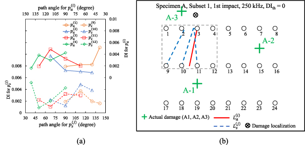
Figure 22. Damage localization results for subset 1 in specimen A under first impact. The driving frequency is 250 kHz and  . (a) damage index for path groups; (b) actual damage locations, preserved mean angle lines and damage localization.
Download figure:
Standard image High-resolution imageAs a summary, if the maximum damage index in a subset is approximately equal to or less than a certain level, say 0.005, it can be concluded that no damage exists within the subset. With  , it might result in a false damage location within the subset or a predicted damage in the exterior of the subset at low accuracy.
4.4.2. Results for a damage within a subset.
Figure 23 shows the DI variations with path angles and the calculation results of damage localization for subset 5 of specimen B. The damage indices are obtained from signals after 1st impact with driving frequency 275 kHz. In subset 5, the four transducers 5, 6, 7 and 8 are assigned as actuators while the four transducers 13, 14, 15, 16 are assigned as sensors. The value of  for this case is 0.141268, as listed in table 5. This value is much greater than the threshold value of 0.005. It indicates that there exists a damage within this subset. In figure 23, it is seen that four path groups are preserved to form four mean angle lines and a predicted damage location is calculated. In figure 23, it is seen that the nearest actual damage is B-2. The damage localization is quite accurate with a dimensionless distance of
  , as seen in table 11.

Figure 23. Damage localization results for subset 5 in specimen B under first impact. The driving frequency is 275 kHz and  . (a) damage index for path groups; (b) actual damage locations, preserved mean angle lines and damage localization.
Download figure:
Standard image High-resolution imageFigure 24 shows the results subset 5 of specimen B. The damage indices are obtained with driving frequency 275 kHz. The difference of this case from figure 23 is that the results in figure 24 are analyzed after the second impact. The damage size of B-2 is greater after 2nd impact. The value of  for this case is 0.499151, which is higher than that for the case of figure 23. By comparing the result for the first impact, the increasing
  for second impact suggests that this parameter can reflect the damage level. The damage localization in figure 24 is also similar to that in figure 23, showing high accuracy in prediction of damage location. The dimensionless distance for this case is
  , as seen In table 11.
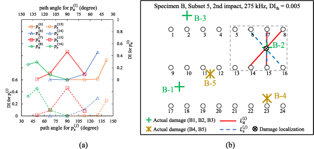
Figure 24. Damage localization results for subset 5 in specimen B under second impact. The driving frequency is 275 kHz and  . (a) Damage index for path groups; (b) actual damage locations, preserved mean angle lines and damage localization.
Download figure:
Standard image High-resolution imageIn one subset with more than one preserved mean angle lines, an intersection point is formed by taking any two of the lines. There may exist more than one intersection points. With the damage localization results shown in figures 23 and 24, it can be concluded that, by applying the two exclusion rules with  within one subset, only one damage can be identified in this subset if the intersection points are distributed in a small region, and the damage can be localized within this region.
4.4.3. Results for a damage near boarder of a subset.
There are two cases for a damage existing near border of a subset. The first is that a damage exists near a transducer of a subset. Figure 25 shows the DI variations with path angles and the calculation results of damage localization for subset 9 of specimen A. The damage indices are obtained from signals after second impact with driving frequency 300 kHz. In figure 25(a), it is seen that the damage indices for path group  are greater than those for path groups pivoted by the other three actuators since the damage A-4 is near actuator 13. The damage indices for paths 13–22 and 13–23 are the largest as these two paths directly hit the damage. However, distributions of the DI's for path groups pivoted by actuators do not fit the Gaussian distribution curves. For the four path groups pivoted by the sensors, the damage index variations fit the Gaussian distributions and are preserved by applying the two exclusion rules. The damage localization results in an accurate damage location prediction with a dimensionless distance of
  .
.

Figure 25. Damage localization results for subset 9 in specimen A under second impact. The driving frequency is 300 kHz and  . (a) Damage index for path groups; (b) actual damage locations, preserved mean angle lines and damage localization.
Download figure:
Standard image High-resolution imageFigure 26(a) shows the DI variations with path angles for subset 7 of specimen B after the second impact with driving frequency 250 kHz. This is another demonstration for a damage existing near a transducer. For the eight path groups, five of them are preserved by applying the exclusion rule 1. For  , one of the five preserved path groups, the peak value of the fitting function is
  . The reference damage index for this subset is
 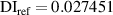 . The damage index ranking plot that is used to calculate this
  value has been shown in figure 4. By further applying the exclusion rule 2 with
  and
and  , it is seen that
  is excluded since
  . By using the four remaining path groups that are preserved, the damage localization results are shown in figure 26(b). It is seen that the predicted damage location is near actual damage B-5 with a dimensionless distance of
  . The damage localization is quite accurate. If the exclusion rule 2 is not applied, the path group
  is preserved, and the damage localization result is also shown in figure 26(b). It is seen that the mean angle line for
  has a large error by comparing other four preserved mean angle lines. It results in a more inaccurate location prediction with
  . In the case study of figure 26,
  dominates the exclusion results by applying the exclusion rule 2 since
  . It suggests that the damage localization can be more accurate if the value of
  that is determined by the procedure shown in figure 4 is utilized.
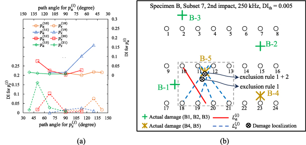
Figure 26. Damage localization results for subset 7 in specimen B under second impact. The driving frequency is 250 kHz and  . (a) Damage index for path groups; (b) actual damage locations, preserved mean angle lines and damage localization.
Download figure:
Standard image High-resolution imageThe second case is that a damage does not exist near a transducer, but near the right or left border of the subset. Two examples will be demonstrated for this case: subset 1 in specimen A at second impact with 275 kHz and subset 4 in specimen B at first impact with 300 kHz. Figure 27 shows the DI variations with path angles for these two examples. For subset 1 in specimen A at second impact with 275 kHz, the damage A-5 is near the left border of the subset, as indicated in figure 8. In figure 27(a), it is seen that no path group is preserved by applying the two exclusion rules. It is obvious that the path 1–9 has the highest damage index of 0.049 97 as it is the nearest path to the damage. For the other path, the damage indices are much less than that for path 1. The second largest damage index in this subset is 0.009 854. The subset 1 is the most left one in the transducer layout, and the path 1–9 is the most left one in the subset 1. Thus, the information shown in figure 27(a) can conclude that a damage exists one the left side area of the subset. This conclusion coincides with the actual location of damage A-5. Similar results can be seen in figure 27(b), where the DI variations with path angles for subset 4 in specimen B at first impact with 300 kHz are presented. The path 7–15, the most left path in this subset, has the highest damage index of 0.1510, while the damage indices for the other paths are much smaller. The variations of the damage index can be accepted since damage B-2 is located one the right border of this subset. Again, no path group in this case can be preserved. The damage B-2 cannot be identified in subset 4, however, it can be identified by the next subset, which encloses this damage.

Figure 27. Damage index distributions versus path angles for (a) subset 1 in specimen A at second impact with 275 kHz and (b) subset 4 in specimen B at first impact with 300 kHz.
Download figure:
Standard image High-resolution imageBy summary, the criterion to identify the case with only one damage near boarder of a subset is similar to the case with only one damage within the subset. The intersection points by applying the two exclusion rules with  are located in a small region.
4.4.4. Results for two damages within a subset.
For second impact in specimen C, there are two damages in subset 9. Figure 28 shows the damage index variations and damage localization results for this subset. The driving frequency and threshold damage index are 250 kHz and 0.005, respectively. By looking at the damage index variations with the path angles as shown in figure 28(a), it is observed that the damage index for path hitting the damage is higher. For example, consider the path group  pivoted at sensor 22. The four paths in this path group are 12–22, 13–22, 14–22 and 15–22. The second path of this path group (13–22) does not hit the damage. The path 12–22 passes near the damage C-1. Both the other two paths, paths 14–22 and 15–22, hit damage C-4. Thus, the distribution of damage index for path group
  reveals its minimum at path 13–22. The damage indices for the other three paths are relatively higher. The path-angle dependent DI variation for path group
  does not follow the Gaussian distribution and has been excluded in the damage localization calculations. For another path group
  , the two damages affect the path-angle dependent DI variation in a similar manner. However, it follows the Gaussian distribution and is preserved after applying the exclusion rule 1. As a result, there are five path groups are preserved and the intersection points formed by the mean angle lines are distributed in a relatively large region. Based on the present algorithm, only one damage location can be reported. In this case, a predicted damage location is obtained at the middle of the two real damages. Nevertheless, the predicted damage location is more near to damage C-4 with
  .
.
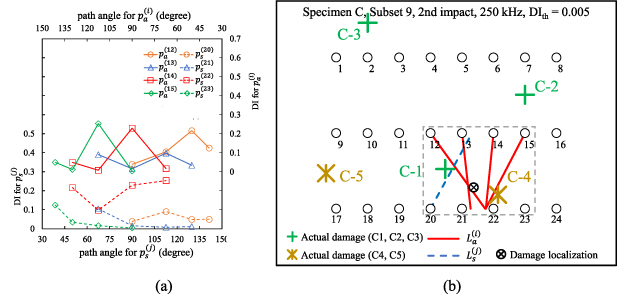
Figure 28. Damage localization results for subset 9 in specimen C under second impact. The driving frequency is 250 kHz and  . (a) Damage index for path groups; (b) actual damage locations, preserved mean angle lines and damage localization.
Download figure:
Standard image High-resolution imageThe damages C-1 and C-4 can be separately predicted by subset 7 and subset 10, as shown in figures 29 and 30. The subset 7 encloses only one damage C-1 and has a predicted damage location with  . Similarly, the predicted damage location by subset 10 is near to damage C-4 with
  . It is concluded that for the case that one subset encloses two damages, these locations of the two damages can be separately identified by the neighborhood subsets.

Figure 29. Damage localization results for subset 7 in specimen C under second impact. The driving frequency is 250 kHz and  . (a) Damage index for path groups; (b) actual damage locations, preserved mean angle lines and damage localization.
Download figure:
Standard image High-resolution image
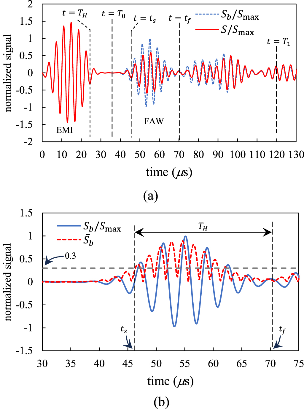
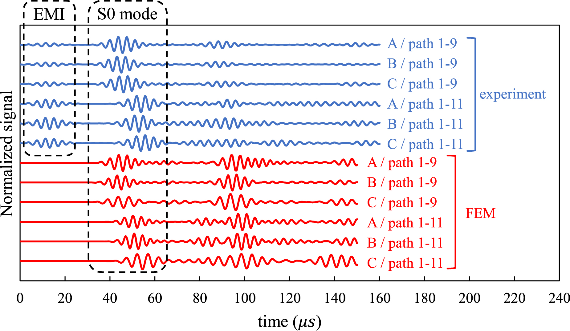
Figure 30. Damage localization results for subset 10 in specimen C under second impact. The driving frequency is 250 kHz and  . (a) Damage index for path groups; (b) actual damage locations, preserved mean angle lines and damage localization.
Download figure:
Standard image High-resolution image
With the observations from figures 28 to 30, a subset is identified that there are two damages within it if the intersection points are distributed in a relatively large region by applying the two exclusion rules with  . The predicted damage may be located between the two actual damages. The localizations for the two actual damages can be obtained from the results of the two adjacent subsets.
5. Conclusions
In this paper, the multi-damage localizations for laminated composite plate is conducted by Lamb waves, which are excited and received by piezoelectric transducers. Three specimens were prepared for testing, each of which has a transducer layout composed of 24 piezoelectric transducers. There are twenty layers for specimen A without taper, while taper designs are used in specimens B and C. The three specimens were put in the drop testing machine to create actual damages. By using the algorithm developed in this study, the locations of multiple damages are identified. The conclusions are as follows.
- 1.Accurate damage localization: The damage localization results show that the damage location can be accurately predicted for the case that a damage exists in the interior of a subset.
- 2.Multiple-damage localization: For a composite plate with multiple damages, their locations can be identified by using multiple subsets.
- 3.Available for tapered composite plate: In theory, the dispersion characteristics depend on the plate thickness. According to the results from experiments and finite element analysis, no significant wave propagation characteristic is found by comparing the three specimens. It means that the same transducer layout can be applied on specimens A (without taper) and the other two specimens (with tapers).
Except for the above conclusions, additional remarks are also given as follows:
- 1.In the experiment, the baseline signals are needed in the damage index calculations. It may increase the measurement complexity. However, the proposed algorithm can be available for baseline-free signals if the distributions of such signals in a path group fit a Gaussian distribution for the case that a damage exists in a subset.
- 2.The signals may be affected by environments such as temperatures or loadings. However, the environmental uncertainties can be included in the proposed model. By taking the temperature variation as the example, a database of the baseline signals measured from various temperature environments can be pre-established. Then this database can be used to compensate the damage index calculation if the temperature varies.
Acknowledgments
The authors appreciate the Aerospace Industrial Development Corporation (AIDC) for the financial support and for providing instruments used in the experiments. The authors are grateful to Gow-Ming Lin in AIDC for his support of the research project management, and Rong-Der Chien, Chun-Yu Wu and Yang-Chih Lin in AIDC, and Professor Yung-Chun Lee in Department of Mechanical Engineering, National Cheng Kung University (NCKU) for their participations in the technical meetings during this research.
Data availability statement
The data cannot be made publicly available upon publication because they contain commercially sensitive information. The data that support the findings of this study are available upon reasonable request from the authors.