

Abstract
The development of energy harvesters for smart wearables is a challenging topic, with a difficult combination of ergonomics constraints, lifetime and electrical requirements. In this work, we focus on an inertial inductive structure, composed of a magnetic ball circulating inside a closed-loop guide and converting the kinetic energy of the user's limbs into electricity during the run. A specific induction issue related to the free self-rotation of the ball is underlined and addressed using a ferromagnetic 'rail' component. From a 2 g moving ball, a 5 cm-diameter 21 cm3 prototype generated up to 4.8 mW of average power when worn by someone running at 8 km h−1. This device is demonstrated to charge a 2.4 V NiMH battery and supply an acceleration and temperature Wireless Sensor Node at 20 Hz.
Export citation and abstract BibTeX RIS
1. Introduction
The functionalization of ordinary objects with embedded electronic systems is a fast-growing trend, commonly referred to as the Internet of Things. This phenomenon is especially visible in the immediate human environment, and 'smart' objects—watches, phones, cars, houses—have become commonplace. The growth of this domain has triggered an interest for energy harvesting solutions to reduce the need for energy storage units, or even to replace them. These electrical generators are designed to comply with the constraints of the application, such as comfort of use (weight, volume), lifetime and cost. Our study focuses on worn-intelligence (or 'smart wearables'), for example pieces of clothing embedded with communicating sensors. In this application, as in greater scales, one typical energy harvesting approach consists in converting the environmental forms of energy, such as light and heat. Various photovoltaic structures are possible, from rigid/flexible modules enabling power densities as high as 10 mW cm−2 [1, 2], to fiber-shaped devices [3–5] with lower conversion efficiencies (up to 7–8%). Body-area thermoelectric systems were also investigated [6–8] and showed electrical powers densities of a few tens of μW/cm2. Both light and heat sources are 'circumstantial': the output of the related devices are dependent on conditions external to the user, respectively irradiance (day/night, indoor/outdoor) and air temperature.
In the field of body-worn systems, especially the smart sportswear applications, another available energy source is the motion of the user. This mechanical input may be converted into electrical power through several different transduction modes. Piezoelectricity describes the conversion of mechanical stresses into an electrical voltage, with devices such as shoe insoles [9, 10] woven garments [11–13] and even joint-activated gears [14]. The deformation of the fabric and the friction between textile layers can be converted using electrostatic capacitor structures polarized by triboelectric effect [15, 16]. Finally, the electromagnetic induction is well-suited to exploit accelerations in inertial generators [17–27].
Among inductive harvesters in the literature, 1D inertial resonant structures were the most widely studied [17–23]. Indeed, this type of device exhibits good performances from the typical 'swing' and 'shock' excitations pertaining to the human motion. However, depending on the orientation and the positioning of the device on the body, only one excitation direction can be exploited, thus limiting the mechanical input [24]. In response, a few 2D and 3D devices were investigated [25–27]. Besides, it was suggested in [25] that non-resonant rolling magnetic harvesters could be especially adequate to the low-frequency, wideband content of human motion. Our study focuses on a non-resonant structure that combines a single magnetic ball moving freely inside a circular loop carried by the user. This shape aims at taking advantage of both mechanical energy from the step impacts and the swing of the limbs, while avoiding as much as possible the 'containment' effect which limits the performance of resonant generators [28].
The sections of this paper are organized as follows: first, the structure of the device and its operation are detailed through analytical and numerical models (section 2); the experimental performances of a prototype are then presented, and alternative device configurations are compared (section 3); finally, the application supplying demonstration with a rechargeable battery and a wireless sensor node is presented (section 4).
2. Looped inertial energy harvester
2.1. Structure
The system consists of a magnetic ball moving freely inside a circular tore. Several independent coils are wrapped along the loop (figure 1). When the system is carried by a person during a physical activity, the magnetic ball moves freely inside the loop and induces electrical currents inside the coils. These outputs are rectified separately and driven to a common charge. A peripheral band (or 'rail') of soft ferromagnetic material is encircling the device (the role of this practical tip is explained in section 2.3).

Figure 1. General structure of the energy harvester.
Download figure:
Standard image High-resolution image2.2. Theory
2.2.1. Model
First, we propose a brief theoretical approach to estimate the potential of this toroidal format to harvest energy from human mechanical excitations. We consider a general 2D model of an inertial system with an eccentric mass  pivoting around a central axis at a distance
  (which in our case corresponds to the radius of the closed trajectory of the ball). The self-rotation of the magnetic ball is not considered here. The model parameters are illustrated in figure 2. In the reference frame of the generator (with the relative coordinate system
  ), the position of the moving mass is defined by an angular parameter
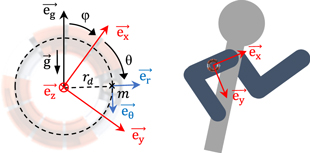
Figure 2. Model parameters.
Download figure:
Standard image High-resolution imageThe device is assumed to be attached 'vertically' to a limb of the user and undergoes an 'in-plane' excitation, characterized by an acceleration  and a rotational acceleration
  for instance, a subject is running with the device attached to the side of his arm (figure 2). The inertial forces trigger the free motion of the magnetic mass, which can be described using Newton' second law (1):
φ is the rotation angle between  and the vertical direction
 and
and  are the acceleration components expressed in the relative (
 ) coordinate system and
  is gravity.
  and
and  are the electromechanical and mechanical damping coefficients, which are arbitrarily considered constant in this theoretical study. The instantaneous electrical power
  extracted from the kinetic energy of the moving mass by the electromechanical damping is:

2.2.2. Simulation from an experimental 'running' input data
Using a 9-axis motion sensor (InvenSense MPU-9250) attached to the upper arm, we recorded both acceleration components 
 (figure 3(a)) and rotational speed
  (figure 3(b)) of the limb while the person was running on a treadmill at 8 km h−1. Interestingly, the rotational measurement shows an asymmetric form, which suggests that the 'upward' swing (corresponding to the negative peaks) plays an important motor role in the running gait. With this experimental input, the previous model was implemented on Matlab Simulink and the output power of the generator was simulated. The moving mass (m = 2 g) and the mechanical damping coefficient (
 = 0.01 N.s/m) were kept constant.

Figure 3. Simulation results, from an experimental input recorded on the arm while running at 8 km h−1. The moving mass m = 2 g and mechanical damping  = 0.01 N.s/m are kept constant. (a) and (b) Detail of the acceleration and rotational components of the input. (c) Average load power and power density as a function of the radius of the device. (d) Dependence of the load power on the electrical damping coefficient
  for three different device radiuses
Download figure:
Standard image High-resolution imageFirst the influence of the radius  of the device was examined (figure 3(c)). For each point, the value of electrical damping
  was determined so as to maximize the average output power. The results suggest that a few milliwatts can be generated from this 'running'-type excitation, for a radius of the device greater than 1 cm, and increase with the radius. This was expected because of the rotational component of the excitation,
  is unaffected by the radius
  (see equation (1)), while the electrical power remains dependent on this parameter (expression (2)). The power density relative to the volume of the toroidal device decreases from 230 μW.cm−3 to 130 μW.cm−3 (the volume
  considered for these values is
  with a tore section
  set to 1.33 cm2).
The impact of the electrical damping was also evaluated, for three different generator radiuses (figure 3(d)). This simulation revealed that smaller device radiuses require greater levels of electrical damping to reach the maximum power. This observation is important since the magnetic mass here is small (2 g), which limits the damping levels achievable. On the other hand, the output power seems less dependent on the electrical damping for smaller device radiuses, which can be an advantage considering that this parameter is difficult to control experimentally due to the self- rotation of the magnetic ball.
2.3. Electromechanical coupling and self-rotation of the magnetic ball
While performing preliminary experiments with this concept of generator, it was observed that the electromechanical damping coefficient—and thus the electrical power—were very limited with the elementary device (i.e. without the additional ferromagnetic 'rail'). We propose here to explain this effect and show how the implementation of a ferromagnetic rail offers a solution, using a finite element method approach (performed on COMSOL). A simplified static situation is considered, involving only one coil and neglecting the curvature of the device (figure 4(a)). The parameters are illustrated in figure 4(b): the ball moves along the y-axis, its magnetic polar axis is assumed in the xy plane and defined by angle  For the numerical values, we consider an 8 mm-diameter N38 magnetic ball (2 g mass), a 1000-turns coil and a 1.55 mm × 0.2 mm ferromagnetic band placed at x = 8 mm (these parameters are the same as for the prototype, see table 1 hereafter). Examples of the magnetic field densities
  produced by the magnetic ball and the coil are illustrated in figures 4(c) and (d), respectively. The geomagnetic field, which is in the order of a few 10−5 T, is neglected in this study.
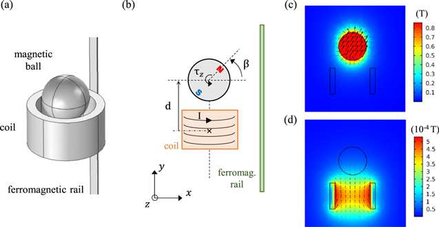
Figure 4. FEM model of the magnetic ball moving relatively to a single coil. (a) 3D geometry of the COMSOL model. (b) Model parameters. (c) and (d) examples of computed magnetic fields generated by (c) the magnetic ball (β = 60°, d = 10 mm), and (d) the coil (I = 5 mA) (the ferromagnetic rail is hidden).
Download figure:
Standard image High-resolution imageTable 1. Prototype parameters.
| Parameter | Value |
|---|---|
| Radius of the trajectory | 2.5 cm |
| Tube inner diameter | 8.6 mm |
| Tube outer diameter | 13 mm |
| Volume | 21 cm3 |
| Mass of the device | 40 g |
| Diameter of the moving ball | 8 mm |
| Mass of the moving ball | 2 g |
| Number of independent coils | 16 |
| Copper wire diameter | 62 μm |
| Number of turns per coil | 1000 |
| Coils resistance | 200 Ω |
| Ferromagnetic rail width | 1.5 mm |
| Ferromagnetic rail thickness | 200 μm |
2.3.1. Magnetic flux gradient inside the coil
As stated by Faraday's laws, induction is linked to the time variation of the magnetic flux inside the coil. Here, this variation is the consequence of both the displacement and the rotation of the ball. The value of the magnetic flux averaged over the volume of the coil is plotted in figure 5. The electrical damping coefficient  is proportional to the square of the instantaneous gradient of this flux [30]. Depending on the signs of the respective variations of the displacement
  and the magnetic orientation
  the sum of the two contributions can either add-up or compensate each other. For example, the ball rolling away from the coil will cause an oscillating magnetic flux inside the coil with a decreasing amplitude.

Figure 5. Average magnetic flux in the multi-turn coil plotted over the distance d between the magnetic ball and the center of the coil, and the magnetic orientation of the ball β.
Download figure:
Standard image High-resolution imageAlthough the addition of soft ferromagnetic parts in inductive generators usually aims at channeling the magnetic flux inside the coils and thus increase the electromechanical coupling [29], given the reduced dimensions of the soft ferromagnetic medium here (the 'rail'), its influence on the magnetic flux density inside the coil is insignificant.
2.3.2. Electromagnetic torque
During the motion of the ball, induced current in the coil produces an opposing magnetic field which slows down the moving magnet. It also applies a magnetic torque,  which triggers the self-rotation of the ball. We evaluated the amplitude of this torque as a function of the instantaneous magnetic orientation
  of the ball and the electrical current I in the coil (figure 6(a)). The torque is proportional to the induced current in the coil, and has different effects depending on the relative motion of the ball. For example, if the magnetic ball is sliding away from the coil, the coil will generate an attractive magnetic field to oppose the motion of the ball. The stable orientation of the latter, defined by
  and
and  will be
  or
or  depending of the sign of the induced current in the coil. On the contrary, if the magnetic ball is sliding towards the coil, the magnetic field produced by the induced current in the coil will be repulsive: the only stable orientation is the induction-less one, i.e.
 ![$\beta =0^\circ \,[180^\circ ].$](https://content.cld.iop.org/journals/0964-1726/26/10/105035/revision2/smsaa8918ieqn41.gif)

Figure 6. FEM torques computation. (a) Torque applied by the coil to the ball, as a function of its polar orientation  and the current
  in the coil. These values were calculated for a distance d = 5 mm between the magnetic ball and the coil. (b) Static torque applied to the magnetic ball by a 1.5 mm-wide × 0.2 mm-thick ferromagnetic rail.
Download figure:
Standard image High-resolution imageIn any case, the induced self-rotation of the magnetic ball tends to limit the magnetic flux variation inside the coil, in accordance with Lenz's law. To counteract this issue, the magnetic orientation of the ball shall be imposed by other effects than this electromagnetic torque.
2.3.3. Ferromagnetic torque
The presence of the nearby ferromagnetic band is not neutral regarding the orientation of the magnetic ball. Indeed, it imposes a preferential direction which corresponds to the polar axis of the ball being perpendicular to the surface of the ferromagnetic (![$\beta =0^\circ \,[180^\circ ]$](https://content.cld.iop.org/journals/0964-1726/26/10/105035/revision2/smsaa8918ieqn44.gif) ), as illustrated in figure 6(b). The corresponding 'static' torque
), as illustrated in figure 6(b). The corresponding 'static' torque  can thus oppose the previous torque from the coil. Evidently, the parameters of the ferromagnetic rail must be chosen to limit the amplitude of this torque, and not permanently set the orientation of the magnetic ball to
  in which case the magnetic flux seen by the coil (and the electrical damping) would remain almost null (see figure 5). Besides, a too important ferromagnetic part would obviously prevent the motion of the ball altogether because of the attraction force (and thus the static friction) it would generate.
2.3.4. Friction torque
The last component that must be taken into account is the mechanical 'rolling' torque resulting from the friction between the casing and the ball during its motion. As an approximation, it may be evaluated using the Coulomb friction model. Considering the normal force  applied on the ball by the inner wall of the tube and using the same motion model parameters detailed in section 1, the norm of this force (3) can be expressed from the equation of motion projected on the radial direction. If the peripheral ferromagnetic rail is present, the radial attraction force
  it applies to the magnetic ball is compensated by the wall.
with:
In Coulomb friction model, the maximum tangential force applicable by the wall to the ball is  μ being the coefficient of friction. Considering the radius of the magnetic ball
  the amplitude of the friction torque is then:

The coefficient of friction between the magnetic ball and a plastic wall was estimated experimentally to μ ≈ 0.2. Using Simulink and the ferromagnetic attraction force calculated by FEM, the average value for the normal wall force  was estimated to be 0.05 N or 0.35 N, without or with the ferromagnetic band respectively. The corresponding values for the friction torque are 4.10−5 N.m and 2.8 10−4 N.m.
2.3.5. Resulting torque—advantages of the ferromagnetic rail
The self-rotation of the ball follows equation (5).  =
=  is the moment of inertia of the ball.

Without the ferromagnetic rail, the electromechanical torque is higher than the friction torque for induced currents of few mA only. In that case, the electrical damping of the device is limited, and the ball is often sliding which increases the mechanical losses. On the other hand, the friction torque becomes a lot higher when the ferromagnetic part is present; adding the 'static' torque generated by the latter, the influence of the induction-limiting torque from the coils is therefore reduced, and the electrical damping is strengthened (at the cost of some static friction). Besides, depending on the instantaneous intensity of the mechanical excitation applied to the device and the dimensions of the ferromagnetic rail, the ball is often rolling which reduces the mechanical losses. By promoting the rolling behavior, the ferromagnetic rail therefore offers a dual advantage.
3. Experimental testing
3.1. Prototype characteristics and rectifying circuit
A prototype was built with a  radius trajectory. The body was manufactured in plastic, and the 1000-turns coils were made on a winding machine (figure 7(a)). The dimensions of the ferromagnetic rail were chosen in order to increase the 'natural' rolling of the magnetic ball sufficiently to overcome the electromagnetic torque, as explained previously. Prototype parameters are detailed in table 1. The signals of the independent coils were rectified separately with voltage doubling circuits, the outputs of which were placed in parallel (figure 7(b)). We used BAS70-04 diodes, with a forward voltage drop of 410 mV at 1 mA.

Figure 7. (a) Picture of the prototype, showing the bound rectifying circuit on top. (b) Schematic of the electrical circuit, with resistive loads.
Download figure:
Standard image High-resolution imageThe moving magnet was one N38 NdFeB ball (Ø8 mm, m = 2 g, Br = 1.24 T). The mechanical (parasitic) damping coefficient  was estimated to be in the 0.005–0.01 N.s/m range from the oscillations of the ball in a free fall experiment (i.e. in open-circuit, without the ferromagnetic band). A value for the average electromechanical coupling
  was also determined by inducing a forced cycling motion of the ball (at a fixed velocity
  ) and measuring the average dissipated electrical power
  according to expression (6):

Without the ferromagnetic rail, this value was evaluated at ce = 0.007 N.s/m, which is very low given the 2 g magnetic mass and the 1000-turns coils. It is in particular insufficient regarding the optimal value (0.05 N.s/m) suggested by the previous simulations of the system. After attaching the ferromagnetic rail to the device, the electrical damping coefficient was estimated to about ce = 0.04 N.s/m, which is closer to the optimal value estimated for this device dimensions (see figure 3(d), with  ).
).
3.2. Electrical performance
We tested the performance of the device while it was carried by a person running on a treadmill. The average electrical power received by the two resistive loads ( ) was measured during 50 s samples.
First, the relevance of the added ferromagnetic strip was verified (figure 8(a)). The device was attached to the arm, and the average power received by the resistive loads was measured for running speeds between 4 km h−1 (very slow) and 8 km h−1 (moderate). The load power of the elementary device varies from 0.5 mW to 0.8 mW, while it ranges from 1.8 mW to 4.8 mW after adding the ferromagnetic band. These last values are consistent with the preliminary simulation (which announced 4.2 mW at 8 km h−1 for the 2.5 cm radius system). The form of the electrical current in the two resistive loads for the device with the ferromagnetic rail (at 8 km h−1) is displayed in figure 8(b). It shows current 'packets' occurring with a frequency of about 2.5 Hz. They are triggered by the step impacts and swing accelerations, happening at this same frequency, which overcome the static friction.

Figure 8. Electrical results in a 2 × 200 Ω resistive load. (a) Average load power of the device with and without the ferromagnetic rail. (b) Shape of the electrical current in the two resistive loads (arm, 8 km h−1). (c) Average load power for different generator locations.
Download figure:
Standard image High-resolution imageDifferent generator locations on the body were tested, revealing significant performance differences between them (figure 8(c)). We exposed in a previous study [23] that the upper body was well benefiting from impacts from both feet during the run, while only half were felt in the legs. The 'upper arm' and 'wrist' positions get mechanical energy from these steps 'shocks', as well as the important limbs 'swing' accelerations. They thus yield the best output powers (between 2 and 5 mW). It is worth noticing that the generator worn on the wrist produces more than 3 mW even at the lowest running speeds. The foot area is also quite relevant because of the important 'swing' amplitude. The two tested orientations of the generator (vertically on the ankle, and horizontally on top of the shoe) showed similar results, from 0.5 to 2.5 mW. However, placing the device around the thigh (for example in the pocket) was not conclusive, with a maximum of 0.6 mW generated at 8 km h−1. This could be expected since both 'swing' and 'shocks' are reduced at this position. The system was finally tested during the walk (at 4 km h−1). This activity is mechanically far less energetic than running, and therefore the output powers were only of a few 100 s μW.
These output powers up to 4.8 mW obtained from the 'running' activity are satisfying given the small moving mass (m = 2 g). Indeed, state-of-the art inertial energy harvesters for human motion with comparable moving mass values usually generate sub-mW outputs [17, 20, 25, 26]. This performance underlines the relevance of the 'looped' device format combined with the rolling moving mass. The power density of the device is in the average, up to 220 μW.cm−3 relatively to the 21 cm3 volume of the whole loop. The best inductive generators in the literature exhibited power densities over 500 μW.cm−3 [22, 23], obtained from resonant structures.
3.3. Variant 1—half-device
To improve the power density, we considered a 'half' device, with extremal foam bumpers (figure 9(a)). The output powers of this configuration are close with those of the full device at the lowest running speeds, as about 2 mW were produced when the device was worn on the arm. At higher speeds however, the motion amplitude limitation decreases the output, and a maximum of 3 mW only was produced at 8 km h−1 (figure 9(b)). The related power densities are only slightly better, up to 280 μW cm−3 (figure 9(c)).

Figure 9. Experimental testing of the 'half device' concept (a) Schematic of the concept. (b) Load power and (c) corresponding power density, compared with the full device.
Download figure:
Standard image High-resolution image3.4. Variant 2—moving magnetic balls trains
Besides the use of the ferromagnetic rail, another solution to keep the electrical damping at a sufficient level is to block the self-rotation of the moving magnetic part. We considered a magnetic 'train' of two magnetic balls separated by a curving spacer (figure 10(a)). The interaction between the balls keeps the magnetic polarization of the moving ensemble constant along the trajectory. From the free-fall experiment, the mechanical damping coefficient associated with this configuration was cm = 0.05–0.1 N.s/m, which is ten times the value obtained for the single moving ball. The use of solid or liquid lubricants was tested, but did not permit to lower this value significantly. Because of it, the output power of the system (carried on the arm) was importantly weakened (between 0.8 mW and 1 mW, see figure 10(c)), despite the greater moving mass (m = 4 g). Although the performance may be improved by using the low-friction materials for the inner wall of the tube and the surface of the magnetic balls, these results suggest that ability to roll of the previous single ball is an important factor to decrease the friction losses.

Figure 10. Characterization of the device with (a) one or (b) two magnetic balls trains. (c) Average electrical power in the resistive loads, while carrying the device on the arm and for different running speeds.
Download figure:
Standard image High-resolution imageThe fixed magnetization orientation enables using two moving magnetic ensembles placed in a repulsive configuration, as illustrated in figure 10(b). However appealing in terms of additional mechanical input, this concept was eventually not conclusive experimentally, as shown by the weak output power (figure 10(c)). A first explanation that could be advanced is that the repulsive force between the two magnet trains effectively limits their respective motion range and subsequently the achievable velocities and power output. However, as observed with the 'half-device' (Variant 1), the reduced motion range should not have been that much of an issue, at least for the lowest running speeds. Yet, we observe that the output power with the two moving 'trains' at 4 km h−1 is only half of what was obtained in the single moving 'train' situation. Therefore, the main explanation for this weak electrical performance lies probably in the mechanical losses. The two magnetic parts interact not only in terms of angular repulsion, but also in terms of torque: the two magnetic dipoles try to rotate to reach a stable magnetic alignment. This interaction increases the mechanical friction with the walls furthermore.
4. Application testing
4.1. Recharge of a NiMH battery
Many applications of energy harvesters require an intermediate storage unit, at least to provide a steady voltage source. The full-loop device with a single magnetic ball (m = 2 g) and the peripheral ferromagnetic rail was tested to recharge a 2.4 V NiMH battery (RS Pro, 80 mAh). For this experiment, the outputs of the rectifying circuits were connected to two 1 mF capacitors, in parallel with the battery (figure 11(a)). The power transferred to the cell was calculated from the average current it received during the experiment, i.e.  This current was measured by monitoring the voltage across a 50 Ω resistance that was connected in series with the battery. The generator was placed on the side of the upper arm. The average charging power increased from 1.5 mW to 2.8 mW, for running speeds from 4 to 8 km h−1 (figure 11(b)).

Figure 11. Charging a NiMH battery. (a) Power circuit, and (b) average transferred power with the device carried on the upper arm, for different running speeds.
Download figure:
Standard image High-resolution image4.2. Power supply of a body-area wireless sensor node
The looped generator was finally tested with a Wireless Sensor Node (WSN) to validate the whole energy harvesting chain. This WSN was made of an nRF51 System-on-Chip with a Bluetooth Low Energy stack (Nordic Semiconductor) and an ADXL363 3-axis acceleration and temperature sensor (Analog Devices), which are both ultra-low power consumption devices (figure 12(a)). The measured power consumption of this node at a 20 Hz operating frequency was 1.2 mW. Compared to the previous cell charging experiment, the device can produce enough power to recharge a battery and fuel the WSN at the same time, which is interesting given the variations of intensity of human activity: the stored extra power may be used during low-activity periods.

Figure 12. (a) Picture of the Wieless Sensor Node (WSN). (b) Power management circuit. (c) Screenshot of the smartphone receiving the collected data via Bluetooth Low Energy, displaying the 3 acceleration axes.
Download figure:
Standard image High-resolution image
We verified that the direct power supply of the WSN was possible. A low-power Schmitt trigger was placed at the output, set to close a PMOS switch as soon as the voltage on the buffer capacitor reaches 3.3 V, and to open it when it falls below 2.5 V (figure 12(b)). This configuration solves the issue of the large power consumption of microcontrollers under 1 V. The good operation of the WSN, sending data at 20 Hz was validated. Figure 12(c) shows a screenshot of the receiving smartphone displaying the measured 3-axes acceleration during the test.
5. Conclusion
We studied an atypical design of kinetic energy harvester dedicated to the human motion, and specifically to the running activity. The combination of the 'looped' format and the rolling moving magnet enables to convert both in-plane accelerations and rotation efficiently. The average output power was about 5 mW in a resistive load while running at 8 km h−1 and wearing the device on the arm or the wrist, which is a good performance regarding the small moving magnet (2 g ball). The system was proven to be application-ready and could charge a 2.4 V NiMH battery at 2.8 mW, or supply a wireless 3-axis acceleration and temperature sensor node measuring and transmitting data at 20 Hz. Future work will focus on alternative resonant architectures of the system, to reduce its dimensions to improve the clothes integration prospects while increasing the power density.