

Abstract
This review article summarizes recent developments related to the dynamical formation of persistent spin helices in GaAs- and CdTe-based heterostructures. We start with fundamental aspects of spin-orbit interaction in quantum wells, in particular the Dresselhaus and Rashba terms and their relation to the bulk and structural inversion asymmetries, respectively. In the regime of balanced interactions, their combined impact gives rise to the formation of the persistent spin helix, i.e., a regime where a unidirectional spin grating with enhanced coherence time is established. The experimental scheme relies on ultrafast Kerr microscopy and permits to excite the spin polarization and detect it with a simultaneous spatial and temporal resolution of micrometers and picoseconds, respectively. For a microscopic understanding and a description of the results, kinetic theory of spatio-temporal spin dynamics of two-dimensional electrons is presented. In addition, Monte Carlo simulations of the spin distribution function are performed. Based on these concepts we discuss three areas with recent advances in the field of spin helices. (i) Anisotropic spin transport and spin helix dynamics in a modulation-doped GaAs quantum well is analyzed. It is observed that application of an out-of-plane electric field changes spin-orbit interaction through the Rashba component and the cubic Dresselhaus term. Remarkably, a weak in-plane electric field substantially increases spin diffusion and also affects the spin helix wavelength. (ii) In-plane magnetic fields applied in two perpendicular orientations allow for the extraction of the individual spin–orbit coupling parameters. (iii) Finally, we explore the influence of optical doping on the spin helix in a CdTe quantum well. Most importantly, a non-uniform spatio-temporal precession pattern is observed. The kinetic theory of spin diffusion allows us to model this finding by incorporating a dependence on the photo-carrier density into the Rashba and the Dresselhaus parameters.
Export citation and abstract BibTeX RIS
1. Introduction
Spin-orbit (SO) interaction in two-dimensional electron gases (2DEGs) is responsible for a broad range of phenomena, including spin Hall and spin galvanic effects [1–5], and spin textures such as the persistent spin helix (PSH) [6–8]. A PSH in (001)-grown zinc-blende-type quantum wells (QWs) occurs when parameters associated with the bulk (Dresselhaus) [9] and structural (Rashba) [10] inversion asymmetries are equal in strength [11–13]. Then, the effective momentum-dependent magnetic field  associated with spin-orbit interaction has a constant direction and can be eliminated by a unitary transformation of the Hamiltonian. This is referred as a restoration of the SU(2) spin rotation symmetry [13, 14] that enables the emergence of a persistent unidirectional spin grating (or helical spin-density wave) [15]. In this balanced regime, the spin relaxation of electrons [16, 17] is suppressed [18] and the lifetime of spin helix is increased by several orders of magnitude [13, 19].
PSH texturing shows promise for spintronic applications, because the Dresselhaus (β) and the Rashba (α) SO couplings can be readily tailored by material choice and device design [20, 21]. For example, two-dimensional electron systems, such as GaAs QWs with modulation doping, are naturally suited to balance α and β by a proper choice of doping and the well width [15]. An external magnetic field  vectorially adds to
  allowing for the reconstruction of the spin splitting in
  -space and the determination of α and β [22]. In addition, electric fields induced by a back gate provide direct electrical control over
  and the spin properties of the system [23–25]. Also dual modulation-doping geometries have been utilized [26, 27] resulting in the demonstration of a stretchable PSH by tuning α and β simultaneously [28]. A moderate in-plane electric field drives a spin helix to propagate [29] uncovering that the electron drift can affect the spin diffusion and the PSH wave vector [30, 31]. Promising theoretical work for the creation of crossed spin helices in double QWs has been reported recently [27, 32]. It predicts a topologically nontrivial skyrmion-lattice in an electron gas as a result of two super-imposed spin helices [33]. More application-oriented publications deal, e.g., with the effect of lateral confinement on the evolution of the spin helix [34].
In this review article, we summarize recent developments related to the dynamical formation of PSH textures in GaAs- and CdTe-based heterostructures. It is organized as follows. In section 2 fundamental aspects of SO interactions in QWs are presented. In particular, we discuss the Dresselhaus and Rashba SO terms and their relation to the bulk and structural inversion asymmetries, respectively. A regime of balanced interactions, where the effective magnetic field points along a certain crystallographic axis, supports the PSH with the wave vector perpendicular to this axis. Section 3 describes the experimental scheme that permits us to excite the PSH mode and to detect the spin polarization with a simultaneous spatial and temporal resolution of micrometers and picoseconds, respectively. In short, we use the spatially- and time-resolved Kerr microscopy with independently tunable pump and probe pulses to raster scan the electronic spin polarization. For an understanding of the results, we present a microscopic theory of the spatio-temporal spin evolution in section 4. The theory is based on the kinetic equation for the spin distribution function. It includes the stochastic walks of electrons in the QW with SO interaction, causing the Dyakonov-Perel spin relaxation, the spin diffusion and the electron drift in an in-plane electric field, the spin rotation in the effective magnetic fields associated with the diffusion and drift, and the Larmor precession in an external magnetic field. In parallel we also perform simulations based on Monte Carlo methods.
Based on the above concepts we then present novel aspects of the PSH physics. Section 5.2 lays out the studies of anisotropic spin transport and spin helix dynamics in a modulation-doped GaAs QW, i.e., the best understood model system for PSH phenomena. It is observed that application of an out-of-plane electric field to the sample changes the spin decay time and SO interaction through the Rashba and the cubic Dresselhaus component. Remarkably, an in-plane electric field also substantially modifies both the spin diffusion and the PSH wavelength. By applying an external magnetic field in the QW plane in the directions parallel or perpendicular to the spin helix we directly quantify the spin–orbit coupling parameters. Section 5.3 explores the influence of optical doping on the PSH in a CdTe QW. Most importantly, a non-uniform spatio-temporal precession pattern is observed. The kinetic theory framework of spin diffusion allows to model this finding by incorporating the photo-carrier density into the Rashba and the Dresselhaus parameters. This work shows universality of the PSH by its observation in a II-VI compound and the ability to fine-tune it by optical doping.
2. Spin-orbit coupling in semiconductors
2.1. Rashba and Dresselhaus spin–orbit coupling
The Dirac equation predicts a coupling of the spin angular momentum of an electron to its orbital motion which is referred to as SO coupling. The coupling leads to the fine structure of atomic levels and the splitting of the valence band to the Γ8 band (with the j = 3/2 total angular momentum) and the split-off Γ7 band (with j = 1/2) in zinc-blende semiconductors like GaAs, see figure 1(a).
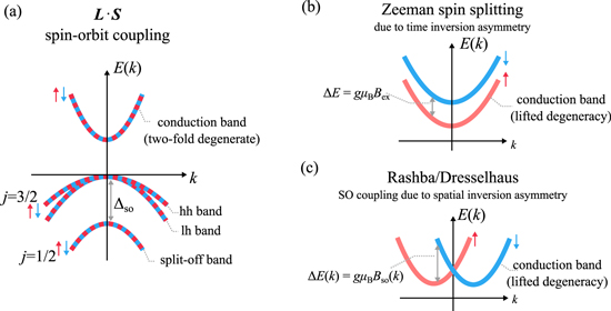
Figure 1. Common types of spin splitting in the band structure. (a) SO splitting of the valence band into the Γ8 band with the angular momentum j = 3/2 and the split-off Γ7 band with j = 1/2 in zinc-blende crystals. (b) Zeeman splitting of the conduction band by an external magnetic field. (c)  -dependent Rashba/Dresselhaus SO splitting of the conduction band.
Download figure:
Standard image High-resolution imageIn semiconductor structures lacking a center of space inversion, the remaining spin degeneracy in the conduction and valence bands is lifted apart from some high-symmetry points in the Brillouin zone. This splitting can be described by a Zeeman-like contribution  to the Hamiltonian, where
  is the operator of magnetic moment and
  is an effective magnetic field dependent of the wave vector
  . Generally, the effective magnetic field may originate from SO coupling in the electric fields of either atoms constituting a non-centrosymmetric crystal lattice (Dresselhaus term) or imposed by an asymmetric heterostructure (Rashba term) [9, 10]. The effective magnetic field is odd in the wave vector
  , which follows from time reversal symmetry and ensures the fulfillment of Kramer's degeneracy
  . We note that, in a centrosymmetric system, space inversion additionally imposes
  . Together with Kramer's degeneracy, it provides
  , i.e., the spin degeneracy holds across the entire Brillouin zone. Therefore, the observation of the spin splitting in the absence of an external magnetic field, which is crucial for the formation of PSH, is restricted to non-centrosymmetric structures. This requirement is met, among other systems, in GaAs and CdTe crystals of the Td point group and QWs based on them [35, 36].
The Dresselhaus Hamiltonian, that describes SO splitting of the conduction band due to bulk inversion asymmetry (BIA), is given by
where  is the material dependent bulk Dresselhaus parameter, σj are the Pauli matrices, and
 ![$x^{\prime} | | [100],y^{\prime} | | [010]$](https://content.cld.iop.org/journals/0268-1242/34/9/093002/revision2/sstab3158ieqn16.gif) , and
, and ![$z| | [001]$](https://content.cld.iop.org/journals/0268-1242/34/9/093002/revision2/sstab3158ieqn17.gif) are the cubic axes. Microscopically, γD can be calculated in the framework of the multiband
are the cubic axes. Microscopically, γD can be calculated in the framework of the multiband  theory using the Löwdin partitioning technique [35, 36] or the tight-binding approach [37]. The results of the calculations for a number of III-V compounds can be found in [37].
For a QW grown along z, the expectation value  vanishes while
  does not and one obtains the effective 2D Hamiltonian [17]

We note that additional SO contributions with the same symmetry properties may arise from interface inversion asymmetry and strain in lattice-mismatched heterostructures [21].
In the following, we discuss the spin dynamics in the in-plane coordinate system ![$x\parallel [1\bar{1}0]$](https://content.cld.iop.org/journals/0268-1242/34/9/093002/revision2/sstab3158ieqn21.gif) and y∥[110] which is natural for (001)-oriented QWs [38]. The Hamiltonian (2) in the new coordinate frame takes the form
and y∥[110] which is natural for (001)-oriented QWs [38]. The Hamiltonian (2) in the new coordinate frame takes the form

It can also be written in the equivalent form

where θ is the polar angle of the wave vector  .
.  , β = β1 − β3 is the Dresselhaus parameter which combines

In the case of a degenerate electron gas, k should be replaced by the Fermi wave vector kF. The Hamiltonian (4) contains the first and third angular harmonics. The contribution of the third angular harmonic is typically small, since β3 ≪ β1, and can be often neglected.
The Rashba Hamiltonian arising from the structure inversion asymmetry (SIA) is given by

In the case of SIA produced by an external and/or built-in electric field  , the Rashba parameter α can be related to the electric field by
  . The parameter γR depends on the QW material and design [35, 36]. The
  theory yields γR = 5.206 eÅ2 and γR = 6.930 eÅ2 for bulk crystals GaAs and CdTe, respectively, [35].
The total effective Hamiltonian of a free electron in a QW, including the spin-independent kinetic energy  with the effective mass
  , the Dresselhaus and Rashba contributions, HBIA and HSIA, respectively, can be conveniently presented in the form

where g is the effective g-factor, μB is the Bohr magneton, and  is the effective magnetic field caused by SO coupling. The field is given by
and contains two contributions  and
and  describing the first and the third angular harmonics, respectively. Most remarkably, the effective magnetic field may be strongly anisotropic in
  -space. This is crucial for the PSH evolution and it will be a major aspect of our work to investigate how the Rashba and Dresselhaus parameters can be extracted and manipulated by indirectly monitoring
  .
.
Neglecting the small contribution  , which is cubic in
  and has a minor influence on the PSH formation, and solving the Schrödinger equation with the Hamiltonian (7) one obtains the energy dispersion

which features a linear dependence of the spin splitting on the electron wave vector  .
.
A cross-section of the dispersion given by equation (9) is depicted in figure 1(c). For comparison, the dispersion in the degenerate case and in the case of Zeeman splitting are sketched in figures 1(a) and (b), respectively. Specifically, the dispersion with the Rashba and Dresselhaus SO coupling implies a lateral shift of the 'spin-up' and 'spin-down' subbands in  -space. Note that the dispersion exhibits an anisotropy in
  -space if both α and β are non-zero. The lateral separation of the spin parabolas in the dispersion cross-section implies the linear increase of the splitting with the wave vector and represents a peculiar characteristic of the Rashba and Dresselhaus SO coupling. The Zeeman splitting in a real magnetic field, on the contrary, corresponds to the spin branches that are vertically separated as depicted in figure 1(b). In figure 1(a), the band structure of a zinc-blende bulk crystal is shown in the absence of external fields and without the Rashba and Dresselaus SO coupling. In this case, the conduction band as well as the valence bands are spin-degenerate.
2.2. The persistent spin helix
The PSH appears as a unidirectional wave of electron spin polarization under the specific condition that the Rashba and Dresselhaus parameters are equal in strength,  at the Fermi level. Here, we consider the experimental situation of an electron spin ensemble created by an ultrashort focused laser pulse. The pulse is circularly polarized and excites electrons with the spins oriented along the QW normal (z). The spin polarized electrons diffuse in the QW plane from the small spot where they have been created. Consequently, a coupling of the electron spins to the effective magnetic fields arises from non-zero
  -values during diffusion. Thus, the diffusing spins undergo precession while they spread in the QW plane. Each electron sees a sequence of individual effective magnetic fields depending on its individual diffusion trajectory. Nevertheless, the overall spin coherence is maintained in the special regime of the PSH, see figure 2(e). This manifests in the characteristic spin texture which emerges due to the combined spin precession and diffusion.

Figure 2. Schematic distribution of Bso in k-space, showing orientation and magnitude of the effective field on the Fermi circle. (a-d) The plots reassemble (a) pure Dresselhaus, (b) pure Rashba and (c,d) ratios of BIA/SIA = 1 and BIA/SIA = 0.45. (e) Apperance of the PSH as unidirectional spin wave indicated by colored arrows (bottom layer). False-color representation of the spin orientation in a two dimensional map (top layer), adapted in part from [22].
Download figure:
Standard image High-resolution imageFrom this observation the question arises of how the spin coherence is stabilized although the spins of individual electrons are affected by different effective magnetic fields during their random walks. To understand it, we consider the structure of the effective field  at α = β. In this regime, the y-component of the
  vector vanishes and the field
  becomes unidirectional and dependent of ky only. As a consequence, only a momentum along the y-axis results in precession while a propagation along the x-axis does not create any effective magnetic field and, thus, does not affect the spin. Moreover, for
  proportional to ky in the first power, the spin rotation angle is fully determined by the electron displacement along y being independent of its particular trajectory. This allows one to eliminate the spin-orbit interaction by a unitary transformation of the Hamiltonian and can be also interpreted in terms of the emerging SU(2) spin rotation symmetry.
A schematic distribution of the effective magnetic field on the Fermi circle is depicted in figures 2(a)–(d) for different combinations of α and β. For pure Rashba SO coupling in panel (b) the distribution forms a vortex while for pure Dresselhaus SO coupling in panel (a) it has an anti-vortex structure. Only in the perfectly balanced regime, the field along the kx axis is entirely gone, see panel (c). The mixed regime in panel (d), with β/α = 0.45 , results in a slightly distorted symmetry of the balanced regime.
As a result of the diffusion-driven spin precession in the effective field  , the initially isotropic spot of spin polarization Sz created by a focused laser pulse evolves into a standing unidirectional helical wave of spin density where the z-component of the spin polarization oscillates along the y-axis. The determined precession length λ0,y can be then used to extract the sum of the Rashba and Dresselhaus parameters since λ0,y in the PSH regime is given by

The excitation of the spin helix mode is efficient only if the spatial width of the initially created spin polarization is smaller than the wavelength λ0,y.
Beyond the  contribution, the effective magnetic field contains the small
  term. The dependence of
  on the direction of
  is described by the third angular harmonic. Therefore, the accumulated rotation angle in the
  field depends on individual electron trajectories and averages out in the diffusion regime. It means that the precession around
  does not contribute to the formation of the PHS but rather is a source of the PSH relaxation [22]. An electron drift induced by an externally applied electric field can change the spatio-temporal spin dynamics in such a way that the
  component cannot be neglected anymore. However, this occurs only in the non-linear regime in the electric field when the drift velocity approaches the Fermi velocity. Therefore, we disregard
  in this paper unless stated otherwise.
An important consequence of the SU(2) spin rotation symmetry for the balanced Rashba and Dresselhaus regime is a significant enhancement of the lifetime of the spin helix [11, 13, 39, 40]. The reason is the suppression of the Dyakonov-Perel (DP) spin relaxation mechanism as the dominant source for spin decoherence. The DP mechanism is based on the precession of individual electron spins in the effective magnetic fields  which change in time following the time dependence of the electron wave vectors [16, 17]. In the regime of the PSH, the spin rotation angle is one-to-one related to the electron displacement in the QW plane independent of its particular pathway between the initial and final points and the spin decoherence in the
  field is avoided. In reality, the SU(2) symmetry is not perfectly realized and the spin lifetime remains finite because of the
  contribution, remaining imbalance of α and β, and other sources of spin decoherence.
3. Experimental methods
The PSH is a phenomenon which appears as a textured spin polarization, evolving in time and space. Therefore, it is of central interest to develop an experimental approach that allows for the detection of spin polarization in a temporally and spatially resolved fashion. Generally, the interaction of polarized light and matter is a versatile process which can be harnessed to locally inject spin-polarized electrons via optical orientation.
Optical techniques are also useful to detect the electronic status and the spin polarization in solids. One promising technique is the magneto-optical Kerr effect (MOKE) that transfers the macroscopic magnetization associated with the oriented spin ensemble into the polarization of linearly polarized light. Here this technique is combined with a pump-probe approach which allows for temporal resolution of picoseconds, much shorter than the typical spin coherence times. Additionally, this ultrafast spectroscopy is carried out with spatially independent, tightly focused pump and probe pulses, resulting in the desired spatial resolution of ∼1 μm.
3.1. The magneto-optical Kerr effect
The Faraday effect describes a rotation of the polarization plane for a linearly polarized light beam which propagates through a transparent medium exposed to an external magnetic field [41, 42]. An equivalent effect was observed in reflection geometry by John Kerr and is therefore referred to as MOKE schematically depicted in figure 3 [42, 43]. Following the approach of [44], the role of the external magnetic field can be replaced by any macroscopic magnetization  in the sample generated, e.g., by optical orientation of magnetic moments μs. The resulting interaction of magnetization and the electromagnetic light wave is described by Maxwell's equations. Here we briefly derive the spectral dependence of the Kerr rotation (KR) angle ΘK in vicinity of an optical resonance. This regime serves as a model for the detection of electron spin polarization in the conduction band of semiconductors.

Figure 3. Magneto-optical Kerr Effect on a magnetized sample, in part adapted from [44]. (a) The incoming probe beam is linearly polarized (red arrow) and can be assembled from equally strong right- and left-circular contributions (orange arrows). (b) Reflected polarization in the case of pure Kerr rotation: the linear linear polarization is maintained but rotated by ΘK due to circular birefringence. (c) Appearance of Kerr ellipticity due to circular dichroism, resulting in unbalanced  contributions (indicated by orange circles of different diameter). (d) Combination of Kerr rotation and ellipticity with tilted main axis of the elliptic polarization and unbalanced
  .
.
Download figure:
Standard image High-resolution imageThe MOKE can be described by Maxwell's equations in a non-magnetic material, i.e., the magnetic permeability tensor is set to the vacuum case. Consequently, only the dielectric permittivity tensor  , remains to mediate the light–matter interaction. If the magnetization and the propagation direction of the light is oriented along the z-axis,
  of an otherwise isotropic material becomes an asymmetric tensor with complex elements
  ij
ij
By inserting equation (11) into the electromagnetic wave equation one obtains two normal modes of the light wave which can be identified as right- and left-circularly polarized. These modes feature different complex refractive index  respectively where ± denotes right- and left-circular polarization. From Fresnel's formulas it is known that a difference in the refractive index will result in different complex reflection coefficients given by
  . The complex reflection coefficient determines the amplitude and phase change for a reflected wave. This manifests either as circular birefringence for the case of a phase difference or as circular dichroism for the case of an amplitude difference. Also a combination of both effects is possible. These scenarios are visualized in figures 3(b)–(d). This figure shows the polarization components before and after the reflection from a magnetized sample. After the reflection the light beam has undergone a Kerr rotation and also exhibits Kerr ellipticity (see figure 3(d)). The former refers to a rotated plane of polarization, if the phase of the two reflected circular polarized waves has shifted. The latter describes the emergence of an elliptical polarization in case the amplitudes of the two circular components are imbalanced after the reflection. The angle of Kerr rotation (KR) ΘK, as well as the ratio of major and minor axis ηK in the elliptical polarization, can be quantified from the off-diagonal elements of the permittivity tensor in equation (11) according to
where ![$n=[{\mathfrak{R}}({N}_{+})+{\mathfrak{R}}({N}_{-})]/2$](https://content.cld.iop.org/journals/0268-1242/34/9/093002/revision2/sstab3158ieqn64.gif) is the averaged real part of the refractive indices
is the averaged real part of the refractive indices  . As the real and the imaginary part of
  can be expected to scale linearly with the magnetization, it can be assumed that Kerr rotation and ellipticity are useful measures to read out the spin polarization which initially gave rise to
  .
.
Equation (12) suggests a pronounced frequency dependence of ΘK in the vicinity of an optical resonance. We further evaluate this dispersion for an isolated two-level system with a transition energy ℏω0. It is assumed that its spin degeneracy is lifted and that the energy splitting of the spin up and down sub-levels amounts to an energy Δ small compared with the transition energy. The Kubo formalism [44, 45] allows to derive the expression
that enables to calculate the spectral dependence of ΘK around the resonance, where both sub-levels have the same transition strength f12 and γhw is the spectral half-width of the transition. The line shape of equation (13) is shown in figure 4(c). It is evident that the KR is favourably measured with the probe de-tuned to the slopes of the resonance.
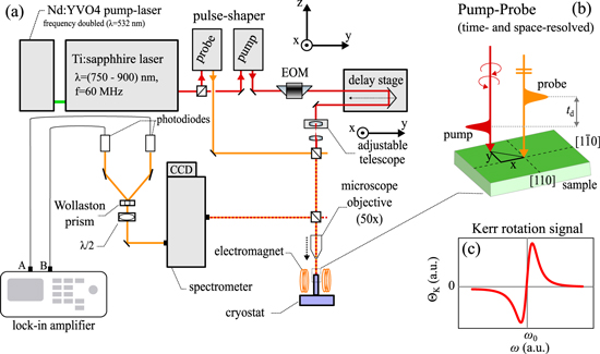
Figure 4. (a) Scheme of the ultrafast Kerr microscope with non-degenerate pump and probe pulses. The pump (probe) is indicated by the color orange (light red). (b) Magnified visualization of the spatial resolution realized on the sample surface where the pump beam can be laterally shifted on the xy-plane. (c) Spectral dependence of the Kerr rotation around a resonance ω0 in accordance with equation (13).
Download figure:
Standard image High-resolution image3.2. The ultrafast Kerr microscope
The use of ultrafast lasers conveniently permits to achieve a temporal resolution in the (sub-)picosecond time domain by using pump-probe techniques. For this method, the output of a pulsed light source is split into two separate pulse trains referred to as pump and probe beams. Subsequently, the pump and probe are recombined on the sample with well-defined polarization, temporal and spatial position. Here, the probe is influenced by changes in the reflection dR caused by the pump beam. Such changes can arise from a variation of the material permittivity, due to the injection of charge carriers and/or a coherent magnetization generated by injected spins [46]. Afterwards, the probe beam is spectrally separated from the pump and directed in a detection scheme which extracts dR/R, often facilitated by lock-in amplifiers referenced to a modulation of the intensity or polarization of the pump beam. The delay time td between pump and probe pulses is set by a mechanical translation stage which allows for the detection of a time-resolved signal dR/R(td).
The experimental setup combines the MOKE with a pump-probe scheme into a Kerr microscope which is depicted schematically in figure 3.1 (a). The output of a mode-locked, femtosecond Ti-sapphire laser with 60 MHz repetition rate is used to provide the pump and probe pulse trains. For spectrally resolved measurements each pulse train is sent through a grating-based 4f-pulse shaper where the pump and probe are individually sliced out from the spectrally broad output of the mode-locked laser [47]. After the wavelength selection for both pump and probe, the temporal resolution of the system is ∼1ps, limited by the chosen spectral bandwidth of ∼0.7 nm. The pump pulse train is sent through a mechanical delay stage and its polarization state is modulated between σ+ and σ− helicities, using an electro-optical modulator (EOM) (QioptiqLM 0202P). The probe is set to linear polarization. In order to record spatially resolved spin dynamics, the pump arm is complemented by a controllable telescope. Lateral motion of the second lens in this telescope enables movement of the pump spot along the x- and y- direction relative to the probe position (see figure 4(b)). Afterwards, both beams are collinearly focused onto the sample, using a 50×objective (Mitutoyo M-Plan APO NIR) which provides a focused spot size for the probe (pump) beams of 1 (3) μm.
In order to minimize spatial fluctuations the sample is nested in a stable helium flow cryostat (Oxford Microstat HiRes2) and cooled to ∼3.5 K. Such cryogenic temperatures suppress phonon scattering as a possible dephasing mechanism and thus help to conserve the coherence of the spin ensemble. An electromagnet positioned around the sample provides variable magnetic fields up to 230 mT in the Voigt geometry. The reflected, non-degenerate pump and probe pulse trains pass a spectrometer (Oxford Shamrock 500i) to filter out the pump radiation. The subsequent detection of KR is based on a Wollaston prism which splits the probe train into two beams with perpendicular linear polarization. These two beams are fed into a balanced detection scheme, converting the KR into an electrical signal using a lock-in amplifier. The detected KR signal depends on the direction of magnetization in the sample. Due to excitation with σ+ (σ−) polarized light the spin magnetization becomes oriented parallel (anti-parallel) to the light propagation direction. The direction of magnetization determines the sense of rotation of the KR and thus the detection of negative or positive signal on the lock-in amplifier. Accordingly, the EOM can be used to impose a temporal modulation to the circular polarization direction of the pump and thus the sign of the pump-probe signal. To this end, the corresponding modulation frequency is sent to the lock-in detection, enabling the measurement of KR angles as small as ∼10 microradians.
3.3. Sample characteristics of CdTe and GaAs quantum wells
The present work is independently conducted in heterostructures made from two prototypical III-V and II-VI semiconductors, namely in GaAs and CdTe QWs. This twofold material choice is of great scientific interest as it allows for a comparison of the PSH characteristics in materials with different SO interaction strength. In addition, PSH physics in II-VI compounds has not been studied extensively [7, 48].
Both crystals are grown as zincblende crystals by molecular beam epitaxy (MBE). The zincblende structure lacks a center of inversion, making it particularly interesting for the study of SO interactions. In general, the strength of the atomic SO coupling is given by the SO coupling constant a ∝ Z/rB3 where the Bohr radius itself is inversely proportional to the atomic number Z. As a result, the coupling constant can be assumed to scale with the fourth power of the atomic number a ∝ Z4 [49]. From this relation a much stronger SO coupling behavior is expected in the CdTe system where the constituent atoms are of higher atomic number than in GaAs:

The extrinsic Rashba SO coupling mechanism is not directly affected by the constituent atoms as it originates from extrinsic potential gradients given by the neighboring layers of the QW. However, the Dresselhaus SO coupling arises from asymmetrically ordered lattice atoms and is thus influenced by the atomic number. However, this dependence is not equivalent with that of the atomic SO coupling constant. A material specific impact becomes present foremost in the Dresselhaus coupling constant γD which can be expected to differ notably between GaAs and CdTe. This difference is backed by theoretical predictions [50] which take into account the band structures of the materials.
Both samples are fabricated as two-dimensional QWs embedded in multilayer heterostructures. The restriction to two dimensions yields a variety of advantages, e.g., a strongly enhanced optical absorption due to an increased oscillator strength of the electron-hole pairs [51]. Moreover, QWs enable a higher degree of spin polarization due to split lh- and hh-bands at the Γ-point [52]. A schematic layer composition and a sketch of the Hall bar structure are displayed in figures 5(a) and (b). In order to create a 2DEG with unbound electrons it is required to lift the Fermi energy into the conduction band, resulting in an electron occupation according to the Fermi–Dirac statistics. A common approach to achieve such a regime is modulation doping. Here, charge transfer from remote dopants into the QW ensures a spatially homogeneous Fermi energy. As a result, a 2DEG in the QW is formed.

Figure 5. (a) Scheme of a typical QW heterostructure of this study. Additional electrons can be transferred from the Si-δ layer into the QW by applying a back-gate voltage. (b) Schematic diagram to illustrate the possible applications of in-plane and back-gate voltages in the Hall bar structure.
Download figure:
Standard image High-resolution image3.3.1. The GaAs heterostructure:
A dQW = 15 nm wide layer of GaAs is sandwiched between two barrier layers made from Al0.33Ga0.67As. The heterostructure is MBE grown on a strongly n-doped GaAs substrate with [001] orientation. The QW is modulation-doped and exhibits a high electron mobility of μe = 2.5 × 105 cm2/Vs as determined from magneto-transport measurements at cryogenic temperatures (∼4 K). From the same measurement an electron sheet density of n0 = 1.3 × 1011 cm−2 is found for the 2DEG. Furthermore, the GaAs QW sample is processed into a back-gated Hall similar to the drawing in figure 5(b) which schematically depicts the Ohmic AuGeNi top contacts utilized for the application of voltage. On the one hand, the application of a gate voltage UBG is a tuning knob for the transverse potential that drops along the QW, enabling a direct manipulation of the Rashba SO coupling via the field  . On the other hand, the gate voltage can be used to tune the electron density within the QW since it drags electrons from an atomically thin delta-layer of silicon dopants (Si-δ) into the QW. Tuning ne has a complementary effect on the β3 Dresselhaus parameter via changes of EF, however, this alteration can be expected to be small compared with the simultaneously occurring change of α. The highly n-doped Si-δ features a donor concentration of 1.9 × 1011 cm−2 and is positioned on top of the QW. Additionally, at the intersection point of the Hall bar electric fields can be generated along the y- ([110]) and x direction (
![$[1\bar{1}0]$](https://content.cld.iop.org/journals/0268-1242/34/9/093002/revision2/sstab3158ieqn69.gif) ) by applying in-plane voltages
) by applying in-plane voltages  and
and  , according to the schematic wiring in figure 5(b).
3.3.2. The CdTe heterostructure:
This sample consists of a dQW = 20 nm wide CdTe QW embedded inbetween Cd0.74Mg0.26Te barriers. The sample is MBE grown on a [001] oriented GaAs substrate. The structure exhibits an exceptionally high quality, enabling the observation of the fractional quantum Hall effect [53]. Post growth, digital modulation doping with Iodine far towards the surface prevents donors from migrating into the QW, warranting a particularly high electron mobility of μe = 4.2 × 105cm2/Vs and a 2DEG concentration of n0 = 3.4 × 1011cm−2 obtained from Hall and conductivity measurements at cryogenic temperatures (∼4 K). Other than the GaAs sample, the present CdTe QW does not have electrical contacts. Therefore, it is neither possible to alter the electron density or  nor to apply drift fields due to the application of voltage. Nevertheless, the results below show that the electron density ne and the emerging PSH in the QW is strongly affected by photo-carriers that can be optically injected into the the conduction band. The table below summarizes the most relevant parameters of the two heterostructures investigated here.
4. Theoretical framework
4.1. Kinetic theory
This section presents a microscopic theory of the spatio-temporal dynamics of a spin ensemble exposed to external electric  and magnetic fields
  . The approach used here is based on an extended version of the drift-diffusion kinetic equation [31, 54, 55]. This differential equation can be solved numerically in order to visualize the formation and decay of the spin helix and compare the results with experimental data. We also provide analytical results for some parameters of the spin density waves such as their decay rates, frequencies, and velocities. Similar results can be also obtained by means of the Green function technique [56, 57] or Monte-Carlo simulations [8].
Kinetic equation that describes the evolution of the spin distribution  in real and momentum spaces has the form

where  and
and  are the spin precession frequency in the external and spin-orbit effective magnetic fields, respectively, and
  is the collision integral. The latter describes the relaxation of the distribution function due to electron scattering by impurities, phonons, and other electrons.
In the collision dominated regime, when  with τ being the scattering time, equation (14) yields the drift-diffusion equation for the local spin density
  [31]
[31]
Here,  is the drift velocity of spin density perturbations, Ds is the spin diffusion coefficient,
  is spin relaxation rate tensor [17],
  is the tensor describing the spin precession at diffusion, and
  is the frequency of the spin precession caused by electron drift [58]. In the relaxation time approximation, the kinetic parameters above have the form


where τ1 is the momentum relaxation time determining the electron gas mobility,  and
and  are the relaxation times of the first and third angular harmonics of the spin distribution, respectively, which are contributed and can be dominated by electron-electron scattering [59–61],
  , and the angle brackets denote averaging with the energy-derivative of the Fermi–Dirac function,
  ,
,  . Note that the drift velocity of spin-density perturbations
  can differ from the conventional drift velocity of electrons
  provided the momentum relaxation time τ1 depends on energy.
For (001)-grown QWs with the effective magnetic field given by equation (8) and the degenerate electron statistics, we obtain

where all the values should be taken at the Fermi level. Note that the second term in equation (21) stems from  [17, 18] while the second term in equation (23) originates from the β3 contribution to β in
  [62].
[62].
4.2. Helical spin waves
We solve the drift-diffusion equation (15) by the Fourier transformation presenting the spin density in the form

there  is the wave vector of the spatial harmonic. The time evolution of the harmonic
  is given by

where the tensor  is defined by
For a given wave vector  the tensor
  has three eigenvalues describing the properties of eigen spin modes. The real part of an eigenvalue determines the decay rate of the mode while the imaginary part determines the mode frequency and velocity. The initial distribution of the harmonics
  can be readily found from the initial distribution of the spin polarization in real space,
  . The integral (24) can be calculated numerically while some general results can be found analytically.
To proceed further with the analytical theory we disregard the  contribution to the effective field and consider first the spatio-temporal spin dynamics in the absence of external fields,
  and
and  . In this case, the matrix
  is Hermitian. All three eigenvalues of
  are real and correspond to the relaxation rates of the spin modes. A minimal value of the decay rate, which corresponds to the longest lifetime, is achieved at a certain finite
  . This wave vector of the long-lived spin waves is directed along y if αβ > 0 and along x if αβ < 0. In the former case, the standing long-lived spin helix is formed from the spin waves with the wave vectors
  with qSH given by [57]
and has the relaxation rate
The polarization of the waves are given by the eigenvectors
revealing their helical structure. Interestingly, at  the lifetime of the persistent spin helix given by 1/γSH is twice as long as the lifetime of the x component of the spin polarization given by 1/Γxx.
4.3. Effect of external fields
When the terms standing for the effects of external magnetic or electric are present in equation (26), the matrix  is no longer Hermitian and has complex eigenvalues. The imaginary parts of the eigenvalues describe the rotation of the spin helix in time and the related phase velocity.
The applied magnetic field induces the Larmor precession for the spin component orthogonal to the magnetic field. For weak fields, the Larmor precession leads to small imaginary parts  of the eigenvalues of the matrix
  which are given by
 ![${\omega }_{{\boldsymbol{q}}}={\rm{i}}{{\boldsymbol{\Omega }}}_{L}\cdot [{{\boldsymbol{s}}}_{{\boldsymbol{q}}}\times {{\boldsymbol{s}}}_{{\boldsymbol{q}}}^{* }]$](https://content.cld.iop.org/journals/0268-1242/34/9/093002/revision2/sstab3158ieqn112.gif) , where
, where  are the corresponding eigenvectors of
  . For the long-lived spin helix with the eigenvector (29) we obtain ωSH = qSH vSH,y with the phase velocity
The group velocity of the spin wave is determined by  . For the long-lived spin helix, the group velocity has the form
and is much smaller that the phase velocity  since α is close to β. Therefore, the external magnetic field applied along the x-axis leads to a motion of the spin pattern with the phase velocity determined by α + β without a considerable shift of the pattern envelope.
In the case of a strong in-plane magnetic fields, the dominant term in the right-hand side of equation (26) is the one describing the spin precession with the Larmor frequency  , where ϕ is the polar angle of the vector
  . There are three eigenvalues of the matrix
  : 0 and ∓iΩ, and three corresponding eigenvectors:
 ![${{\boldsymbol{s}}}_{{\boldsymbol{q}}}^{(0)}=[\cos \phi ,\sin \phi ,0]$](https://content.cld.iop.org/journals/0268-1242/34/9/093002/revision2/sstab3158ieqn120.gif) and
and ![${{\boldsymbol{s}}}_{{\boldsymbol{q}}}^{(\pm )}=[-\sin \phi ,\cos \phi ,\pm {\rm{i}}]$](https://content.cld.iop.org/journals/0268-1242/34/9/093002/revision2/sstab3158ieqn121.gif) . Taking into account other terms in the right-hand side of equation (26) as a perturbation and neglecting the mode mixing we obtain the dependence of the eigenvalues on
. Taking into account other terms in the right-hand side of equation (26) as a perturbation and neglecting the mode mixing we obtain the dependence of the eigenvalues on 
The minimum of the spin relaxation rate is achieved for the modes  at
at ![${{\boldsymbol{q}}}_{\mathrm{SH}}=\mp (2{m}^{* }/{{\hslash }}^{2})[(\beta -\alpha )\sin \phi ,(\alpha +\beta )\cos \phi ]$](https://content.cld.iop.org/journals/0268-1242/34/9/093002/revision2/sstab3158ieqn124.gif) , i.e., in the direction determined by the polar angle
, i.e., in the direction determined by the polar angle

The spin helix has the phase speed

and the relaxation rate
Figure 6 shows the dependence of the direction of the long-lived spin helix on the magnetic field orientation for two different ratio between α and β. When the magnetic field is rotated, the spin helix direction rotates in the same direction if  and in the opposite direction if
  , see the red and blue curves, respectively. The dependence ΦSH (ϕ) is strongly nonlinear: The spin helix direction is 'pinned' to its natural axis in the absence of the magnetic field. The closer the absolute values of α and β are, the stronger the pinning is, see red and blue curves. However, the spin helix is always oriented perpendicularly to the strong magnetic field if the field is applied along the
 ![$x\parallel [1\bar{1}0]$](https://content.cld.iop.org/journals/0268-1242/34/9/093002/revision2/sstab3158ieqn127.gif) or
or ![$y\parallel [110]$](https://content.cld.iop.org/journals/0268-1242/34/9/093002/revision2/sstab3158ieqn128.gif) axes.
axes.
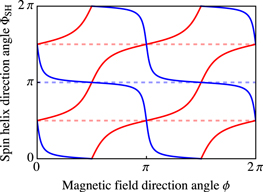
Figure 6. Dependence of the angle ΦSH defining the spin helix direction on the magnetic field orientation angle ψ in strong magnetic fields. The functions are plotted after equation (36) for (α − β)/(α + β) = 1/3 (red curve) and −10 (blue curve).
Download figure:
Standard image High-resolution imageFinally, we consider the effect of an external electric field on the spin helix evolution. We note that the second term in the right-hand side of the drift-diffusion equation (15) can be eliminated by switching to the reference frame moving with the drift velocity  . In such a frame, the effect of the electric field is limited to the drift-induced spin precession with the frequency
  and, in fact, is equivalent to the action of the magnetic field. Repeating the calculations which are done above for the case of a weak magnetic field and returning back to the reference frame we obtain the phase velocity of the spin helix in the electric field

The current-induced spin precession of quasi-stationary electron distribution has been studied in [62].
4.4. Monte Carlo simulations
Complementary to the kinetic theory another approach for the theoretical simulation of spin dynamics is based on the Monte Carlo (MC) method. In general, the MC method is commonly used in computational algorithms as it permits to solve deterministic problems where the need for complex calculation can be bypassed through a large number of random sampling. In comparison with the analytical solving of a differential equation a MC simulation demands a much higher expense in computational calculations. However, often times MC based algorithms can be formulated with much less effort since the calculation of complicated physical effects can be avoided in favor of random sampling. To simulate the spatio-temporal dynamics of a spin ensemble, the diffusion of the spin-afflicted electrons is modeled as the result of consecutive elastic scattering events with a randomization of the electron's direction. Recent publications have shown that the MC algorithm is a suitable tool for the validation of the PSH evolution in general [63] and as well for rather minute features predicted by theory [62, 64, 65].
The specific MC algorithm employed here accumulates the iterative pathway of up to 1 × 10⁶ electrons, traveling with the a constant Fermi velocity which is given by the electron density as  . Assuming the electron velocity to be constant is a reasonable approach within the Fermi–Dirac regime where the occupied states for non-localized carriers are restricted to a small energy band around the Fermi energy. For increased temperatures where this energy band is smeared out a distribution of velocities, in accordance with the Boltzmann statistics, must be applied. Figure 7(a) visualizes a schematic random walk in the QW plane where the electron experiences an elastic scattering event after having traveled for the free mean path l = vFτ given by the scattering time. The scattering time is individually drawn from an exponential distribution
  where
where  is the momentum relaxation time of individual electrons. This sampling accounts for the fact that the time inbetween two scattering events exhibits a stochastic variation. The momentum relaxation time can be obtained from the experimentally observed spin diffusion coefficient given by
  . As a result of scattering, the wave vector
  of the electron is rotated on the two-dimensional Fermi circle in k-space depicted in figure 7(b) and hence the electron changes its direction. The rotation of the wave vector is approximated by a random rotation angle φ taken from a uniform distribution from π to −π. The effective magnetic field, seen by the electron spin during the unperturbed propagation between two scattering events, is taken as constant. However, recalling equation (1) it has been shown that Rashba and Dresselhaus SO coupling is momentum dependent and consequently
  will change together with the wave vector after each event of scattering. Therefore, it is necessary to calculate the three-dimensional rotation for each spin polarization vector
  individually. The axis of rotation is given by the effective field vector
  that acts as a torque on the spin momentum for each iteration i as
where  is a standard three-dimensional rotation matrix which rotates a vector around the axis
  by the angle θ = Ωsoτ. The angle of rotation is the accumulated Larmor precession between to scattering events. Within the MC simulation the resulting vector of spin polarization is tracked together with the current position and wave vector of each electron. Hence, the spatial position of each iteration step is obtained from

After a certain number of scattering events N the Sz component of spin polarization and the spin position is transferred to a two-dimensional false-color plot which displays the spin polarization in dependence on the spatial position for a time td = N · τ after the excitation. Modeling the Gaussian laser beam profile the initial position (x0, y0) of each spin is randomly sampled from a Gaussian distribution around the origin with a FWHM equivalent to the spot size of the laser. Due to a large number of electrons the bins in the false-color plot are filled up with the sum of all z spin components  assigned to the specific area covered by the bin.
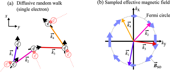
Figure 7. Fundamentals of MC simulations of the PSH evolution. (a) Schematic random walk of a single electron with a changing spin orientation indicated by a black arrow. Its wave vector experiences a redirection due to each scattering event indicated by a star-like symbol. The corresponding reorientation of the wave vector on the Fermi-circle is illustrated in (b).
Download figure:
Standard image High-resolution image5. Results on the formation and manipulation of the PSH
5.1. Emergence and description of the PSH
The section is meant to accustom the reader to the preparation of data developed to visualize the SO coupling mechanisms that drive the measured PSH spin texture. Furthermore, it is discussed how the parameters that are relevant for the PSH are extracted. The section is concluded with a first quantification of the Rashba and Dresselhaus parameters and their validation via simulations based on both the MC method and kinetic theory. Measurements of spin polarization are performed by means of the MOKE effect, allowing for the extraction of Sz from the angle of Kerr rotation. Representing the space and time resolved Sz(x, y, t) data as false-color plot has proven to be an effective way to visualize the PSH. Here, a red to blue color scale indicates the spin polarization component Sz perpendicular to the QW plane, and the in-plane axes are chosen as ![$x\parallel [1\bar{1}0]$](https://content.cld.iop.org/journals/0268-1242/34/9/093002/revision2/sstab3158ieqn142.gif) and y∥[110]. According to section 2.2, the PSH is expected to appear as an unidirectional wave of spin polarization driven by the diffusive expansion of the electron ensemble. A first prediction of the resulting pattern has been developed in figure 2(e) where a parameterization with the spatial wavelength λ0,y has been suggested.
and y∥[110]. According to section 2.2, the PSH is expected to appear as an unidirectional wave of spin polarization driven by the diffusive expansion of the electron ensemble. A first prediction of the resulting pattern has been developed in figure 2(e) where a parameterization with the spatial wavelength λ0,y has been suggested.
This behaviour can indeed be observed in the experiments as shown in figure 8 for the GaAs sample. The three false-color plots in this figure exemplify different ways of how the PSH can be observed, starting with a two-dimensional (2D) map in space depicted in figure 8(a). This 2D map is taken for a constant back-gate voltage of −1.00 V and captures the diffusive status at a fixed delay time of 840 ps. In line with the theoretical expectation the initially oriented spin polarization has not just expanded diffusively in space but has formed an oscillating pattern along the y-axis, indicating a rotation of Sz caused by  . The temporal evolution of the PSH can be tracked by means of the spatiotemporal false-color plots in figures 8(b) and (c) along the x- and y- axes, respectively. Such spatio-temporal maps are composed from single line scans of Sz in dependence of the spatial position. A subset of such line scans taken for different delay times are shown in figure 8(d) along the y-axis. It becomes apparent that the spin polarization expands in space while an additional decay mechanism weakens the signal for long delay times. Moreover, the initial Gaussian shape remains intact over time and no oscillating features are present along the x-axis. However, along the y-axis the initial Gaussian spin distribution, shown in figure 8(d) for the time overlap at 0 ns, develops distinct oscillations on the micrometer range. This spatial anisotropy in the pattern is readily explained by the effective magnetic field distribution in k-space

adapted from equation (8). This expression implies zero magnetic field for electrons that move along the x-axis in a regime of balanced Rashba and Dresselhaus SO coupling. The observed PSH evolution is in excellent agreement with previous studies in similar structures and the line slices along y at a fixed delay time can be described by the fit function
which combines the Gaussian solution of the spin diffusion equation with a cosine modulation by the spin precession length  , corresponding to a characteristic distance for a spin to undergo one full rotation. While the position of the oscillation pattern is determined by the cosine phase parameter y1 the spatial parameter yc denotes the center of the Gaussian spin polarization in space. The fit function describes line scan data at a fixed delay time. All effects of spin decay, diffusion, drift and precession can be integrated into the temporal change of the fit parameters A0, w, yc, and y1. The transparent color lines in figure 8(d) represent best fits of equation (41) to the individual slices of the corresponding spatio-temporal map along the y-axis. Returning attention to the 2D map in panel (a), it is seen that the blue colored PSH stripes are somewhat curved. This fact indicates that BIA and SIA are not entirely balanced. This feature is discussed below, see figure 16.

Figure 8. Evolution of the spin polarization pattern in the GaAs QW mapped out in space and time as false-color plots. (a) 2D map of the PSH for a fixed delay time of 840 ps. (b-c) Spatio-temporal measurements for the x- and y-axis with the respective other coordinate fixed at zero. (d) Exemplary, normalized line scans taken from (c) for different delay times. The colored lines represent best fits to equation (41).
Download figure:
Standard image High-resolution imageThe focus shall now be shifted towards a more quantitative description of the phenomenon with a parameterization by means of the introduced fit function for Sz(y). In order to compare SO coupling in the GaAs and CdTe QWs, extracted fit parameters for both materials are shown in figure 9 (note that the 2D data for CdTe are shown in figure 10). Figure 9(a) depicts the spin precession length as a function of the delay time. For both materials,  decreases in time which is not covered by the static expression in equation (10). However, it has been shown that such a dependence originates from the gradual evolution of the spin distribution from a narrow Gaussian spin distribution at short delay times towards a single mode oscillation at long times [63]. This finite-spot size effect results in a gradual variation of
  to the PSH mode wavelength
  , that is described by
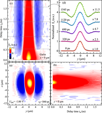
Figure 9. PSH parameters extracted from various 2D maps in GaAs and CdTe. (a) Temporal evolution of the spatial precession length together with best fits to the theory. The predicted value for λ0,y is indicated by dashed lines. (b) Diffusion-induced expansion of w2 together with linear fits. The extracted diffusion coefficient for GaAs is shown in (d) for different gate voltages. (c) Spin lifetimes and (d)spin diffusion coefficients for various backgate voltages. The grey lines are a guide to the eye.
Download figure:
Standard image High-resolution image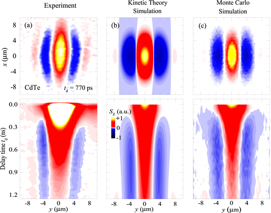
Figure 10. 2D map of the PSH in CdTe for 770 ps and the corresponding spatio-temporal evolution along the y-axis. (a) MOKE measurements of Sz(x, y) (taken from [48]). (b) Simulations based on numerical calculations of kinetic theory. (c) MC simulations.
Download figure:
Standard image High-resolution imageThus, the value of  observed at a specific delay time depends on the initial spot size w0 and the diffusion coefficient Ds [48]. Figure 9(a) shows experimental data for
  together with a fit to this equation. It reveals the PSH mode to be λ0,y = (5.6 ± 0.1)μm for CdTe and
  for GaAs. The corresponding values of (α + β) resulting are (3.19 ± 0.05) meVÅ for GaAs and (4.55 ± 0.08) meVÅ for CdTe. At first glance the difference in between CdTe and GaAs is not very distinct, however, a general comparison should be performed on the level of the Dresselhaus coupling constant γD to rule out the dependence of α and β on sample specific parameters such as the electron density and the QW thickness. This discussion is postponed to section 5.2.1 where the BIA and SIA parameters are determined individually. Furthermore, the space- and time-resolved measurements allow for the extraction of the spin diffusion coefficient Ds by tracing the squared spatial width w2(t) of the Gaussian envelope function with time. Corresponding data for both samples are shown in figure 9(b). In particular, the expected linear time dependence
  of the squared width is utilized to extract of Ds = (50 ± 10) cm2 s−1 for CdTe and (54.0 ± 0.8) cm2 s−1 for GaAs. Assuming the 2DEG to be degenerate at 3.5 K facilitates the calculation of the individual electron momentum relaxation time
  from the theoretical relation
  . The resulting values are noted in table 2 together with other sample specific parameters. EF depends on the carrier density and, thus, on the backgate voltage. In the regime displayed in 9(d) the carrier density varies by a factor of ∼3. The experimentally observed change of Ds depicted in figure 9(d), however, is much weaker and only a tuning by ∼30% is seen. This discrepancy can be accounted for by the fact that the 2DEG can not be treated as degenerate gas but is rather in an intermediate regime towards the non-degenerate statistics.
Table 2. List of sample parameters extracted from the PSH characterization for both materials. For CdTe a short and a long living decay time are observed.
 (μm) (μm) |
Ds (cm2/s) | w0 (μm) | [α + β] (eVÅ) | Ts (ps) | EF (meV) | τee (ps) | |
|---|---|---|---|---|---|---|---|
| GaAs | (11,2 ± 0.2) | (54.0 ± 0.8) | 3.62 | (3.19 ± 0.05) | ∼2200 | 3.05 | 0.6 |
| CdTe | (5.6 ± 0.1) | (50 ± 10) | 3.87 | (4.55 ± 0.08) | 1350/170 | (9.0 ± 0.1) | 0.3 |
Beyond the spatial parameters  and Ds, the investigation of spin lifetimes is of peculiar interest. It is expected that the SU(2) symmetry, which gives rise to the PSH, creates a regime that is extraordinarily robust against spin decoherence caused by the DP mechanism. The spin lifetime of the PSH is extracted from the temporal decay of the fit function amplitude parameter A0. It is important to distinguish the exponential loss of spin coherence and the fact that the amplitude is decreased by spins that diffuse away from the spot of excitation. A combination of these two contributions results in the expression
With the extracted values for Ds and  , the spin lifetime Ts is obtained from best fits of equation (43) to the delay time dependence of A0(td). Figure 9(c) shows Ts for a range of back-gate voltages, with a maximum value of ∼2.2 ns seen for UBG ≈ −0.5 V. A peak-like tuning of lifetimes around a certain gate voltage has been predicted and observed in different studies [13, 18, 19, 31, 40]. This finding reflects the variation of the Rashba parameter α that depends on the electric field
  and is thus directly influenced by UBG. However, later figure 17(e) shows that the ratio α/β converges for back-gate voltages below −1.0V, approximately. Therefore, the decrease of lifetime on the left hand of the peak (from −0.5 V to −2.0 V) is attributed to the strong depletion of the QW as a result of the rather high, negative back-gate voltage.
A comparison of equation (40) with the k-space anisotropy in figure 2(a) shows a clear dependence of the SU(2) symmetry robustness on the level of balance between α and β. As this symmetry suppresses the DP mechanism and therefore leads to very long spin lifetimes, the lifetime peak is assumed to appear for a voltage where α is tuned as close as possible towards β. This finding justifies the choice of UBG = −1.00 V for all following measurements. This specific voltage represents a trade-off in-between a long-living PSH regime and a strong Kerr rotation signal. The KR signal itself is altered by UBG via a density-dependent resonance shift, affecting the optical detection (see figure 4(c)) In conclusion, the fundamental parameters of the PSH in GaAs and CdTe are now mapped out and listed in table 2.
We now turn attention to the theoretical modeling of the 2D maps based on the approaches in sections 4.1 and 4.4. Figure 10 depicts three sets of a 2D (x, y) and spatio-temporal (y, t) maps. The sets represent one measurement of the CdTe sample and two simulations that utilize the CdTe parameters from table 2. Although only the sum of Rashba and Dresselhaus parameter is known so far, the required individual parameters can be calculated with theoretical value of β in table 1. However, for the simulations given here the individual parameters are taken from a later section, see table 3, to obtain the best agreement with the experiment. Figure 10(a) shows the status of the PSH after 770 ps delay characterized by the same unidirectional spin helix wave as in GaAs, however, with a shorter spin precession length. This finding of the Larmor precession pattern, confirms the predominant appearance of Bso for electrons that move along the y direction and is validated by both simulated 2D maps. A similar strong agreement is found by visual comparison of the spatio-temporal maps generated from the measurement (a) and simulations (b, c).
Table 1. List of sample parameters provided by the sample suppliers or assembled from literature if indicated. The Dresselhaus parameter are calculated from equation (5).
| dQW (nm) | μe (cm2/Vs) | n0 (cm−2) | γD (eVÅ3) | ma(m) | β1 (meVÅ) | β3 (meVÅ) | |
|---|---|---|---|---|---|---|---|
| GaAs | 15 | 2.5 × 10⁵ | 1.3 × 10¹¹ | (9–11)a | 0.067c | 4.82 | 0.22 |
| CdTe | 20 | 4.2 × 10⁵ | 3.4 × 10¹¹ | 9.10 ± 0.84b | 0.094c | 2.2 | 0.5 |
Table 3. Overview of the extracted Rashba and Dresselhaus parameters. Results from Salis et al [63] in a 12nm wide GaAs/AlGaAs QW are given for comparison.
| Material | [α + β] (meVÅ) | [−α + β] (meVÅ) | α (meVÅ) | β (meVÅ) | g |
|---|---|---|---|---|---|
| CdTe (this work) | (4.08 ± 0.33) | (0.63 ± 0.01) | (2.35 ± 0.17) | (1.73 ± 0.16) | 1.6 |
| GaAs (this work) | 2.94 | 1.15 | 0.90 | 2.05 | −0.29 |
| GaAs [63] | 4.8 | 0.3 | 2.25 | 2.55 | −0.17 |
While the general reproduction is successful and thus suggests the model to be accurate some smaller deviations can be identified. Firstly, the polarization stripes of the experimental 2D map are visibly more curved than in both simulations. Therefore, this curvature is not explained by an imbalance of α and β only, because such an effect is taken into account in both simulations. It therefore seems more likely that the curvature is a feature that arises from spatially varying SO coupling which will be discussed in-depth later on in section 5.3. Secondly, for short delay times in panel (a) the experimental Sz appears much larger than in the simulations in panels (b-c). This observation suggests a much faster decline of the spin polarization at the beginning of the experiment for td < 300 ps. Indeed, a secondary, fast exponential decay with a lifetime of 170 ps is seen in A0(td). This finding cannot be attributed to thermal effects due to the fairly long time scale. However, a variety of effects can account for short-lived contributions in the present system. For instance, it cannot be ruled out that an unwanted spin polarization with short lifetime is injected into the substrate where it distorts the spin signal which comes from the QW. Another effect could arise from a high photo-carrier density at the temporal overlap, increasing inelastic scattering rates and spin-spin interactions. Such effects for short delay times are not included in the simulations and thus are a reasonable explanation of the encountered differences. Finally, a two-fold decay that is related to the finite-spot size effect is generally expected. Due to the initial transformation of a Gaussian spectrum into the single PSH mode an additional short decay arises at the beginning of the measurement. For longer delay times, the decay is dominated by the pure PSH lifetime which is discussed in the end of section 2.2.
Simulations performed with parameters for GaAs are available in [31] for a sample similar to the one used in this work and show remarkable success in reproducing the experimental data.
5.2. Manipulation of the PSH
The focus is now shifted towards manipulation and control of the spin polarization within the PSH. Therefore, a variety of different control knobs are consecutively investigated and their effects are quantified. Starting with the application of magnetic fields, the influence of back-gate voltage is studied and the PSH is exposed to in-plane electric fields in order to introduce spin drift. The latter case is of interest as peculiar effects on the SO coupling parameters have been reported in recent literature. However, the nature of the related changes, visible in the spin precession length, is not yet fully understood. Hence, special attention is paid to the dependence of λ0,y on the in-plane electric field strength for which contradicting trends are claimed in [30, 31, 62]. Besides the application of external magnetic and electric fields, the SO coupling is strongly affected by the injection of photo-excited carriers into the 2DEG of the CdTe QW. This finding enables an all-optical approach towards PSH control.
5.2.1. Manipulation by in-plane magnetic fields
The characteristic spin texture of the PSH is shaped by effective magnetic fields oriented along the QW plane. Here, we add an additional external magnetic field  (note that again y∥[110] and
 ![$x\parallel [1\bar{1}0]$](https://content.cld.iop.org/journals/0268-1242/34/9/093002/revision2/sstab3158ieqn159.gif) ). Figures 11(a)–(c) illustrates the effect of different applied magnetic field strengths on the spatio-temporal evolution of the PSH in the GaAs sample. The spin helix without external manipulation [panel (a)], evolves symmetrically around the origin. An additional external magnetic field Bex,x, however, imposes a temporal spin precession with a Larmor frequency of
). Figures 11(a)–(c) illustrates the effect of different applied magnetic field strengths on the spatio-temporal evolution of the PSH in the GaAs sample. The spin helix without external manipulation [panel (a)], evolves symmetrically around the origin. An additional external magnetic field Bex,x, however, imposes a temporal spin precession with a Larmor frequency of  . This temporal precession at a fixed spatial position is also referred to as spin beating [67]. Such spin beatings are visible in figure 12(e), where the time dependence of Sz at position (x, y) = (0, 0) is depicted in for an applied magnetic field of 230mT. A best fit with an oscillating, single exponential decay function reveals the Larmor frequency. From this transient, a g-factor of g = −0.29 is determined for the GaAs QW, consistent with the expected increase of the g-factor from the value of −0.44 in bulk GaAs [68–70]. Equivalent measurements in the CdTe sample yield a g-factor of 1.6, in line with other experiments on the same structure [48, 71].
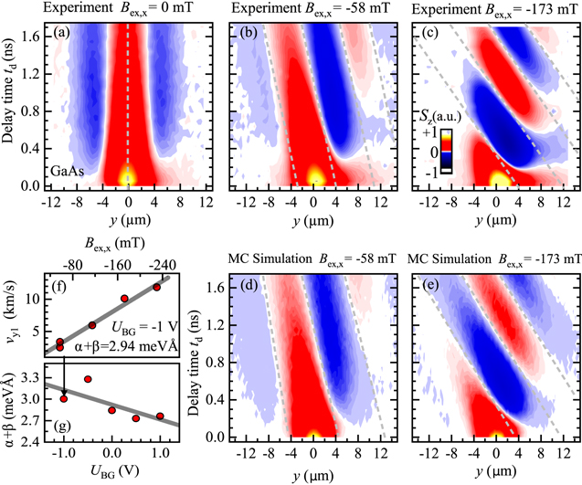
Figure 11. Spatio-temporal evolution of the PSH in GaAs traced along the y-axis for different external magnetic field applied along the x-direction. (a-c) Field-induced tilt of the PSH visualized as grey dashed lines. (d-e) MC simulations of the spin texture for the same experimental parameters as in (b), (c). (f) Dependence of slope of the tilt on  . (g) Parameter (α + β) for various back-gate voltages UBG.
Download figure:
Standard image High-resolution image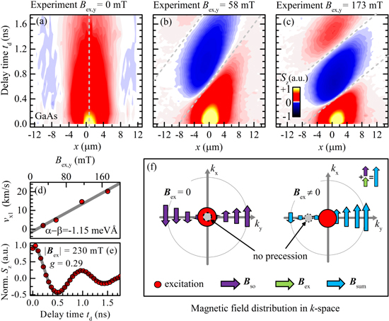
Figure 12. (a-c) Spatio-temporal evolution of the PSH in GaAs traced along the x-axis for different external magnetic fields applied along the x-direction. They grey, dashed lines illustrate the tilted stripe pattern and correspond to a velocity of vx1. (d) Dependence of the phase velocity vx1 on  . (e) Exemplary line scan with magnetic field-induced spin beats for a fixed spatial position at (x, y) = (0,0).(f) Schematic concept of PSH manipulation by means of external magnetic fields with the resulting magnetic field illustrated in k-space.
Download figure:
Standard image High-resolution imageThe spatio-temporal measurements in figures 11(b) and (c), the external magnetic field seems to tilt the PSH stripes over time. As guide to the eye, this tilt is highlighted by grey, dashed lines in the plot. From a comparison of panel (b) and (c), a steepening of the tilt is observed with increased field strength. Generally, the tilt represents an electron velocity for which the spin precession phase is constant. This is equivalent to a fixed spin orientation for electrons that travel with a certain average momentum. As a result, the effective fields have to cancel the external field. Reformulating equation (40) with  , this holds true for a phase velocity of

in agreement with equation (35) for  , i.e. ϕ = 0. The experimental values of vy1 range up to several km/s and can be obtained from a linear fit to the delay time dependence of y1.
This concept of PSH manipulation by external magnetic fields is sketched in a more visual manner in figure 12(f) where the magnetic field distribution in k-space is shown along the ky-axis for the cases with (on the right) and without (on the left) external field. Without an external field, the effective magnetic fields, illustrated by the arrows, grow in magnitude along the y-direction. The photo-injected electron ensemble is centered at k = 0 and the position, where no Larmor precession occurs, is also found at k = 0. When superimposing an external magnetic field, the position in k-space for which no net field acts on the electron spins is shifted from ky = 0 to some finite k-value. Diffusing electrons that exhibit this specific k-value will, therefore, not undergo Larmor precessions but maintain their initial spin orientation.
The application of different magnetic field strengths along the x-axis, exemplified by the two measurements in panel (b) and (c), and the subsequent extraction of vy1 facilitates the determination of (α + β). Specifically, a linear regression based on equation (44) is used to obtain (α + β). A value of (α + β) = 2.94 meVÅ is found, in good agreement with the value in table 2 determined from the spin precession length. Moreover, measurements in the presence of external magnetic field are used to study the influence of the back-gate voltage on α and β. The acquired data is shown in figure 11(g) and reveals a clear trend for a decrease of (α + β) with increasing UBG. An impact of of the back-gate voltage is generally expected as it modifies both β3 via the carrier density and α via the electric field along the QW. This influence is investigated in more detail in section 5.2.3.
The proposed explanation for the observed tilt in the PSH stripes is confirmed by corresponding simulations based on the MC method. For this purpose, the Larmor precession is added to the precession in the effective magnetic field. The false-color plots in figures 11(d) and (e) agree well with the experimental observations, shown in the panels above. The entire set of measurements presented for GaAs in figure 11 is also repeated for the CdTe sample. A value for (α + β) close to the value given in table 3 is found. However, for CdTe the MC simulations show significant dissimilarities with the corresponding experimental data. We later attribute this finding due to the influence of optically induced carriers. The corresponding data are postponed to section 5.3 where this impact of optical doping is studied.
So far external magnetic fields along the x-axis have been applied. This orientation allows to weaken or enhance the effective magnetic fields seen by the electron spins that are recorded in spatio-temporal maps along the y-axis. In contrast, by applying an external field along the y-direction it is possible to access (α − β) from spatio-temporal measurements. Such data are shown in figures 12(a)–(c). A visual inspection suggests a stronger tilt of the PSH stripes compared to analogous panels of figure 11. The fit function in equation (41) is used again for the spin distribution along the x-axis. In contrast to the fit function used along the y-axis the spin precession length along the x-axis now reads

It is determined by the difference of Rashba and Dresselhaus parameter. Accordingly, a much longer wavelength is expected since their difference is supposed to approach zero for a perfectly balanced PSH regime. For a quantitative analysis, the temporal dependence of the x1 parameter is extracted (note that x1 now replaces y1 in in equation (41)) the difference (−α + β) can be extracted from the relation for the x-axis phase velocity vx1 that, in analogy to vy1, takes the form

see equation (35) for  , i.e. ϕ = π/2. Figure 12(d) confirms this linear dependence on the external magnetic field. Moreover, the significantly increased velocities compared with vy1 are in agreement with the assumption of a PSH regime where the SO coupling parameters are similar. From a best linear fit it is possible to quantify (−α + β) = 1.15 meVÅ and to calculate the individual parameters α = 0.90 meVÅ and β = 2.05 meVÅ. The ratio of α/β ∼ 0.5 points to an imperfect PSH regime. However, the results so far show that even in such case the characteristic spin helix pattern is still distinct enough. In retrospect, this unbalance is responsible for the convex curvature in the 2D map of figure 8 [57]. Values for the CdTe sample are incorporated as well in table 3 and exhibit a ratio of α/β ∼ 1.35. In summary, the level of balance in the CdTe sample is slightly higher than in GaAs.
5.2.2. Manipulation by in-plane electric fields
While the application of magnetic fields affects mostly the spins' magnetic moments, the diffusive motion of the spin carriers remains unperturbed. Within this section it is discussed how the spin texture is manipulated by in-plane electric fields along the x- and y-axis. Recently, the effect of electric fields on the PSH evolution has raised special interest due to contradicting observations with respect to the dependence of λ0,y on the field strength. While earlier investigations of Altmann et al [62] report an unchanged spin precession length it has been seen by Kunihashi et al [30] and Anghel et al [31] that λ0,y varies with electron drift, however, with opposite trends. Below we revisit this topic and propose an increased 2DEG temperature due to bias-induced heating as tuning mechanism for the PSH. In the same line of experiments, we address the observation by Altmann et al [62] that the spin precession angle that stems from the cubic Dresselhaus parameter is a factor of two larger for drifting electrons than for diffusing ones. As a consequence, a temporal spin precession appears even in the absence of external magnetic fields. From the related precession frequency the cubic Dresselhaus parameter β3 becomes accessible.
When an in-plane electric field is applied, the photo-injected electron ensemble will start to drift according to the electron mobility. We refer to the emerging spin texture as a drifting persistent spin helix (DPSH). We start with a drift motion along the y-axis. A sequence of 2D maps, capturing the temporal evolution of such a DPSH, is depicted in figure 13. The formation of the characteristic PSH stripe pattern is clearly visible while the center of spin polarization drifts towards negative y-values due to the applied electric field of  (note that an inversion of the electric field leads to inverted but otherwise very similar 2D maps). Comparing the DPSH series with the snapshot of the stationary PSH in figure 8(a) it is apparent that the DPSH features a larger number of oscillations. This observation already points to enhanced diffusion which further spreads the Gaussian envelope in the case of the DPSH.

Figure 13. Apperance of the drifting persistent spin helix (DPSH). Series of false-color 2D maps, tracing the spatial expansion of a spin-polarized electron ensemble into a PSH pattern while the entire spin package drifts in an electric field along the y-axis. The color scale is individually adapted in each map for better visibility. In the bottom right corner the effective magnetic field distribution in k-space is shown schematically. The scheme describes the situation for fields applied along the x-axis but can be qualitatively adapted to the y-axis by flipping the axis.
Download figure:
Standard image High-resolution imageThe temporal evolution of the DPSH for a constant electric field of  is shown as spatio-temporal false-color plot in figure 14. It visualizes the formation of oscillations induced by effective magnetic fields and a continuous shift of the spin package towards negative y-values with increasing delay time. The center position of the spin distribution, given by the yc parameter of the fit function in equation (41), is marked as black dashed line and suggests a continuous shift of ∼17 μm during the time interval of 1.8 ns. Furthermore, there is a clear tilt of the individual stripes highlighted by five parallel dashed lines in grey color. Such a tilt implies a slowly rotating spin orientation with temporal, angular frequency ωc for a fixed spatial position. This is noteworthy, as a fundamental feature of the PSH is its constant precession phase for a certain point in space, being responsible for the formation of the unidirectional spin wave pattern. The tilt is preserved even for large delay times and thus the decrease of the spin precession length (see equation (42)) as a result of the finite-spot size effect can be ruled out as possible explanation. This tilt can, however, be modeled as a temporal precession frequency in addition to the spatial precession already described. For this purpose, the introduction of a slightly changed fit function is favorable, which reads
It permits to study the cosine phase  independently from
  while all other parameters maintain their original meaning. Employing this fit function to DPSH data yields a promising coincidence of theory and experimental line scans, illustrated in figure 14(e) where exemplary data are given for a delay time of td = 1758ps. The analysis of all line scans in panel (a) reveals the trend depicted in panel (c). The center position yc of the Gaussian envelope depends linearly on time, readily explained by a constant drift velocity
  . The slope gives a velocity of 9.86 km s−1, which is much smaller than the Fermi velocity vF = 128.4 km s−1. This drift velocity reveals an electron mobility as high as μe = 6.5 × 105 cm2/Vs which is a bit larger than the mobility extracted from magneto-transport measurements taken at a different back-gate voltage (see table 1).
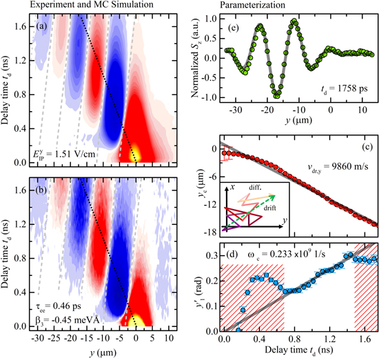
Figure 14. Spatio-temporal appearance and parameterization of the drifting PSH for an applied field of  . (a) Experiment: false-color representation of a DPSH with center positions represented by the black dashed line. The drift-induced tilting of the stripes is indicated by grey dashed lines. (b) Corresponding MC simulations. (c) Center positions yc of the electron ensemble and linear fit to the data. The inset illustrates a diffusive random walk of an electron. (d) Time-dependent phase parameter of the fit function, exhibiting a linear trend in the area which is not greyed out. A linear fit reveals the temporal precession frequency ωc. (e) Exemplary Sz (td = 1785ps) cutout line from the (a) panel with corresponding fit curve.
Download figure:
Standard image High-resolution imageThe tilt of the DPSH stripes in the spatio-temporal map is understood as the electron motion due to both diffusion and drift. Using the expression for the phase velocity of the drifting spin helix equation (37) and the relation  we obtain

For spins under the simultaneous influence of drift and diffusion, the cubic Dresselhaus term leads to an effective spin-orbit interaction beyond simple superposition of these two transport phenomena. For example, when drift and diffusion contributions are parallel, the electrons have large absolute k-values on average. Cubic scaling of the effective magnetic fields with k leads to stronger spin–orbit coupling than the mere sum of drift- and diffusion-related terms As shown in [62] one outcome is that motion due to drift leads to twice the spin precession angle than for diffusion over the same distance. This phenomenon leads to a temporal spin precession at any fixed position, described by the phase velocity in equation (48). By fitting the spatio-temporal data presented in figure 14 with the fit function in equation (47), the time dependence of  is obtained, see figure 14(d). A clear linear trend of the data is given only for a limited time period around 1ns and a linear fit is performed to this data, neglecting points in the hatched regions. As a result, a frequency of ωc = 0.233 × 10⁹ s−1 is obtained, yielding β3 = 0.140 meVÅ. This value is in good agreement with the predicted theory value 0.135 meVÅ that is obtained by inserting the 2DEG density of 0.8 × 1011 cm−2 into equation (5).
Having gathered a full set of parameters, a MC simulation can be created and compared to the experiment. Figure 14(b) depicts MC data created for a diffusion coefficient of Ds = 100 cm2 s−1, yielding a scattering time of τ = 0.46 ps. This value of Ds can be extracted from the linear expansion of w2(td) in the spatio-temporal experiment analogous to figure 9(b). It is noteworthy, that this spatial spread occurs about twice faster than observed in measurements without electric field. Indeed, further experiments with a variable electric field strength confirm such a tuning of the diffusion coefficient, see discussion in [72]. The tilted stripes are attributed to different contributions of β3 depending on electron motion due to either diffusion or drift. The MC simulation provides a general proof of this theoretical model as the tilt of the stripes is well reproduced. However, the value of β3 which gives the best match with the experiment is 0.45meVÅ which is approximately 4×larger than the experimental estimate. Considering the limited data range in figure 14(d) for extracting β3, the discrepancy arises possibly due to uncertainty in the experimental data.
The next set of experiments studies the dependence of the PSH on the strength of the in-plane electric field. Special attention is paid to the behavior of the diffusion coefficent and the SO coupling parameters. The false-color plot in figure 15(a) illustrates a set of Sz(y) line scans taken along the y-axis for a variety of moderate electric fields  , oriented along the same axis. All measurements are taken for a fixed delay time of 1525ps, allowing for the best trade-off between signal strength and advanced PSH evolution. The plot reveals a clearly increasing spatial shift of the spin distribution towards negative (positive) y-values with raising the positive (negative) electric field strength. This shift is explained by the linear dependence of the drift velocity
  on the applied field. The false-color plot appears to be symmetric around
  . This is confirmed by the extracting the yc parameter for each line-scan. Here, the yc parameter represents the center of the spin ensemble and can be translated into the drift velocity via
  ). The resulting data on
  is depicted in figure 15(e) and points to a mobility of 0.38 × 106 cm2/Vs, i.e., close to those in table 1 observed at a slightly different back-gate voltage. In accordance with equation (48) the value of β3 is accessible from the linear dependence of the cosine offset parameter
  on the drift velocity, if the delay time is fixed. Figure 15(g) presents the field dependence of
  . Note that the field strength is converted into a drift velocity by using the results of panel (e). Taking into account the uncertainty of the cubic Dresselhaus parameter, encountered in the spatio-temporal measurement and simulation (see figure 14: β3 = (0.1 − 0.45) meVÅ), the extraction of
  has to be executed with caution. The trend is linear on first sight, confirmed by a linear fit of the entire data set. However, more accurately two linear regimes can be distinguished in the plot and evolve symmetrically around zero velocity. One regime represents a strong increase in the range up to 1500 m s−1 while a second regime is identified for higher velocities with a somewhat smaller slope. Two separate fits allow to estimate β3 = (0.15 ± 0.08) meVÅ albeit with a large statistical error. Despite this, the ambiguous behavior of
  and the dissimilarity of MC simulation and experimental value in figure 14 points to inadequcies of the applied fit function. It is possible that the limited number of oscillations along the x-axis causes errors in the extraction of the
  parameter. Additionally, it is expected that the application of current to the system induces heating of the electron gas, causing a transition to a non-degenerate gas. In this case, the Fermi energy has to be replaced by a higher, average kinetic energy
  . This effect is elaborated thoroughly around formula equation (49) from where it can be seen that heating results in an increase of β3. This finding is in contradiction with the slope in figure 15(g) that rather exhibits a decrease of β3 for increased voltages.
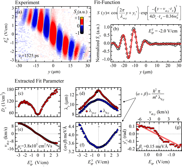
Figure 15. Effect of variable in-plane electric fields on the PSH for a fixed delay time of 1525ps. (a) False-color representation of line-scans along the y-axis for a variety of in-plane electric fields along the same axis. Dashed lines in grey color visualized a shortening of the precession length confirmed in (d). (b) Examplary line scan together with a fit according to the given function. (c-e,g) Dependence of the fit parameters on the applied electric field strength. (f) Tunability of summed Rashba and Dresselhaus parameters with electric field derived from the spin precession length given as blue data points in (d).
Download figure:
Standard image High-resolution imageFitting of the field resolved data performed with equation (47) traces the evolution of the width w of the drifting spin polarization. The diffusion coefficient is then estimated from the expression  . The corresponding data for Ds is presented in figure 15(c). A strong enhancement of the diffusion with rising field strength is evident for drift along ±y. For positive fields, Ds increases monotonically to 180 cm2 s−1 while negative fields raise the diffusion coefficient to a maximum and fields below −2 V cm−1 lead to a decrease. The general increased diffusion is in agreement with the value of Ds = 100 cm2 s−1 that was needed in the MC simulation of figure 14 to reproduced the experiment at 1.51 V cm−1. Precise knowledge about this variation of Ds is also important for the correct extraction of (α + β) from the precession length
  , see figure 15(d). The experimental data reveal a clear, symmetric trend towards a shorter precession length
  for increasing field strength. This is also seen in the false-color plot in figure 15(a) where tilted dashed grey lines are included for visual guidance. This finding suggests a variation of the Rashba and Dresselhaus parameters by fairly weak in-plane electric fields. The symmetric shape of the data around zero field implies that the trend is not an artifact that stems from cross-couplings of the various contacts. Note that figure 11(g) has already shown the impact of back-gate voltage on the SO coupling parameters. Therefore, unwanted cross-coupling of back-gate voltage and in-plane voltages appear possible. This behaviour could result in a simultaneous detuning of the gate voltage by changing the in-plane electric field. However, in such a case the wiring of the sample would lead to a non-symmetrical behavior of λ0,y. Consequently, the decrease of the precession length has to emerge from real changes in the SO coupling parameters.
For a quantitative analysis, one has to distinguish between  and
and  . The former parameter states the transient wavelength of the spin polarization which still develops into a PSH. The latter describes the stationary PSH mode for
  . The relation of both entities is given by equation (42). In particular, the diffusion coefficient strongly influences the temporal evolution of the precession length. As Ds itself is affected by the electric field, it has to be ruled out that the observed change of
  is a secondary effect caused by variations of the diffusion. To this end,
  is calculated and plotted next to the experimental precession length
  in figure 15(d). It is apparent that the resulting
  remains strongly field-dependent. Then the sum of Rashba and Dresselhaus parameter is calculated from equation (42) and depicted in figure 15(f). A substantial increase of (α + β) from 3.35 meVÅ up to ∼4.4 meVÅ for a field strength of ∼ ± 3 V cm−1 is monitored. An unwanted tuning of the back-gate voltage is again unlikely due to the symmetric increase for negative and positive fields. Consequently, it is assumed that the out-of-plane field and thereby α are constant. Therefore the remaining parameters β1 and β3 have to be (indirectly) affected by the applied in-plane bias. β1 is unlikely to be altered by the weak fields. In contrast, the cubic Dresselhaus parameter β3 is known to depend on the the Fermi energy (see equation (5)), that might undergo a significant change if the 2DEG evolves into a non-degenerate gas. In this case, the Fermi energy has to be replaced by the energy
  averaged with the energy-derivative of the Fermi–Dirac function,

where  for electron temperature Te ≪ EF and
  for EF ≪ Te. Such an approach has been successfully applied in a recent study [30]. However, it is incapable of explaining an increase of (α + β). From equation (49) it is obvious that heating will inevitably lead an increase of
  , resulting in a larger β3. At the same time, an increased β3 will always decrease the Dresselhaus parameter β = β1 − β3 and leads to a reduced (α + β), contrary to the data of figure 15(f). Besides this, the absolute change of β3, needed to reproduce the variation of Δ(α + β) ≈ 1meVÅ, would require a temperature variation of several hundreds of Kelvin. In the work of Passmann et al the possibility of such an electron gas heating up to 350 K is discussed in more detail, implying a heat-induced change of Δβ3 ≈ 1.5 meVÅ [72].
The presented experiments so far have been conducted with electric fields applied along the y-axis where λ0,y is relatively small. The Hall-bar geometry of the GaAs sample (see figure 5) facilitates the application of in-plane bias along the x-axis as well. This is of particular interest since, so far, in this direction no significant spin precession is observed as  is much larger. However, signatures of the effective magnetic field can be revealed by the application of magnetic fields, yielding (−α + β) = 1.15 meVÅ which corresponds to a spin precession length of
  for the x-axis, i.e., much larger than the typical diffusion lengths. In order to access information about the PSH from the x-axis it is useful to add electric fields and thus cover the distances needed to observe SO induced precessions. Figure 16(a) shows that this approach indeed reveals a spin polarization wave. In this measurement the spin ensemble is dragged towards negative x-values by a positive field of strength
  , imposing a drift velocity of
  . Analogous to previous y-axis measurements,
  is extracted from the dependence of the Gaussian center parameter xc on delay time. This linear dependence is indicated as black dashed line in figure 16(a). The employed fit function for x-axis line scans is the same as shown in equation (47) for the y-axis. The trend of an enhanced diffusion with increasing field amplitude is confirmed in panel (a). Due to the relatively high fields, needed to induce spin oscillation along the x-axis, the field range for the extraction of Ds shown can be extended in comparison to figure 15. For an applied field of 6.95 V cm−1 an extremely large diffusion coefficient of Ds = 374 cm2 s−1 is observed, corresponding to a seven-fold enhancement when compared to the case without field.
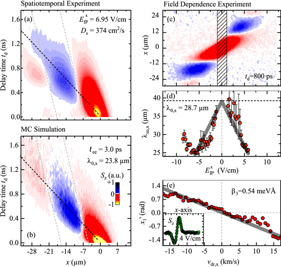
Figure 16. Analysis of the DPSH evolution recorded along the x-axis. (a) Spatio-temporal measurement as false-color representation for field applied along the x-axis. (b) corresponding MC simulation. (c) Field-dependence of the DPSH at fixed delay time and y = 0 μm depicted as false-color plot. (d-e) Parameters extracted from the false-color map above: (d) spin precession length  , (e) cosine offset parameter
  . The inset in (e) shows an exemplary cut out line from (c) with fit.
Download figure:
Standard image High-resolution imageThe diffusion coefficient together with all other parameters extracted from figure 16(a) are confirmed when used to create a MC simulation. The resulting plot is depicted in figure 16(b) where a striking match with the experiment is achieved. On the right hand side of figure 16, a selection of measurements and extracted parameter in dependence of a variable field  is compiled. Figure 16(c) represents a false-color plot of the PSH at td = 800 ps for fields up to ±12 V cm−1. This plot is equivalent to the y-axis measurement in figure 15. For the chosen delay time, oscillations do not become visible for fields lower than
  . This limit is imposed by the fixed delay time which can not be arbitrarily increased because at some point the electrons start to drift beyond the detection window.
Fitting the data to equation (47) reveals the field dependence of the spatial precession length  . An example of successful fitting is given in the inset of figure 16(e). Note that the error of the extracted parameters suffers from the less pronounced oscillation compared to y-axis data. Similar to the observed behavior of
  along the y-axis (see figure 15) a downward trend of
  is found for increasing field values. Along the y-axis a symmetric and linear decrease of
  with absolute field strength is visible, starting from a maximum at zero field (see figure 15(d)). Accordingly, the corresponding trend along the x-axis is modeled with a function
  , allowing for an indirect approximation of
  which can not be directly accessed. The best fit which is plotted on top of the data points in figure 16(d) gives B1 = 39.08 μm, which transforms into
  , taking into account the diffusion coefficient for
  from table 2. This estimation of
  is in good agreement with (−α + β) = 1.15 meVÅ determined from measurements with in-plane magnetic fields, suggesting a value of
  . Another parameter that provides valuable information about the SO coupling is the cosine offset parameterfor the x-axis presented in figure 16(e). Here, the
  , i.e., drift velocity dependence of
  , enables the extraction of β3. For this purpose, the same model developed for the tilt of stripes in spatio-temporal maps, caused by an unbalance in precession due to drift and diffusion, is used. In the preceding analysis the drift velocity dependence of the cosine offset parameter, given in equation (48) has been discussed. As a result, a significant discrepancy of experiment β3 ∼ 0.14 meVÅ and MC simulation β3 ∼ 0.45 meVÅ is found for the y-axis. The analogous data along the x-axis show a clearly linear behavior and, indeed, the extracted value of β3 = 0.54 meVÅ is closer to the MC simulation. This improvement is attributed to a weaker influence of the finite spot size effect. This effect causes a strong alteration of
  with delay time while the broad eigenmode spectrum of the Gaussian distribution develops into a single mode PSH (see discussion below equation (42)). Due to the larger precession length this effect is not so distinct along the x-axis and therefore the extraction of the cosine offset is not strongly perturbed by changes of the cosine frequency which is namely
  . In conclusion, the cubic Dresselhaus parameter remains somewhat uncertain. A combination of values generated from spin transport along both axes, the MC simulation and the theoretically calculated values provide a range of (0.29 ± 0.20) meVÅ for β3. For the given density of n0 = 1.3 × 1011 cm−2 a Dresselhaus constant of γD = (14 ± 10) eVÅ3 is calculated from the experimentally determined cubic Dresselhaus parameter. This finding is in agreement with the range of theoretically expected literature values given in table 1.
5.2.3. Manipulation via the back-gate voltage
The GaAs sample provides a back-gate that can be used to alter the electric field along the growth direction of the heterostructure and across the QW. At the same time, the gate controls the electron density ne in the modulation doped QW by varying the ionization of the Si-δ doping layer outside of the QW. Note that we have investigated the dependence of the spin lifetime on the back-gate voltage in earlier work [39]. So far the impact of the back-gate voltage is briefly touched in figure 9(c) where a peak-like tunability of the PSH lifetime is shown. This section will further quantify the Rashba and Dresselhaus parameter in a regime with variable back-gate voltage.
It is expected that the Rashba parameter is directly affected by a change of the potential drop along the QW, entering into α. Between the two Dresselhaus contributions a differentiation must be made since β1 is expected to be unaffected by UBG. On the other hand, β3 exhibits a direct dependence on the carrier density.
Figures 17(a) and (b) compare the spatio-temporal evolution of the PSH for both ends of the voltage spectrum which is applicable to the sample (UBG = +1.0 V and UBG = −1.75 V). The two false-color plots reveal the characteristic appearance of oscillations in the spin polarization during its diffusive expansion along the y-axis. A difference in the oscillation wavelength of a PSH is observed, see the two parallel, dashed lines and the arrows that serve as a guide to the eye. This observation at first glance is confirmed by further measurements and an upward trend is extracted for λ0,y along the y-axis. The corresponding data points, shown in figure 17(c) as green triangles, are generated individually from a spatio-temporal measurement. Similarly, figure 17(c) shows a decrease of λ0,x as red dots. This trend represents the spin precession length extracted perpendicular to the x-axis. For this axis smaller effective magnetic fields act on the electron spin. Both trends are phenomenologically modeled with an exponential function in order to facilitate further calculations based on the dependence of the SO coupling paramters on UBG. The opposite behavior of λ0,y and λ0,x is best understood from the fact that the former precession length is determined by the sum (α + β) whereas the latter one is dictated by the difference (β − α) of the SO coupling parameters. Consequently, these sum and difference values in dependence on the back-gate voltage can be calculated by inserting the obtained exponential fit functions from panel (c) into equations (42) and (45), respectively. They are shown in figure 17(d) where a growing difference and a diminishing summed value can be identified. This behavior agrees well with the previously made assumption that a variation of α is the dominating effect when the back-gate voltage is changed. Knowing the sum and difference of α and β, the individual values can be determined and are plotted in figure 17(e). It is evident that α decreases while the back-gate voltage is increased and β remains rather constant even though a slight decrease in the blue line is visible. A 60% change of α is evidenced and is comparable to previous studies [40, 73]. For a more detailed description, values for β3 are added to the plot in panel (c) as orange line. These values are calculated from inserting the back-gate voltage-dependent carrier density (data not shown) into equation (5). The carrier density can be directly accessed from the spectral width of the 2DEG Photoluminescence which serves as an experimental measure for the Fermi energy. The strong variation of the cubic Dresselhaus contribution is remarkable as it offers a fine tuning for the PSH. These results are confirmed by similar findings of gate control based on β3 [25].

Figure 17. Control of the PSH with a back-gate voltage. (a-b) False-color plot representations of spin polarization measurements that cover the spatio-temporal evolution of the PSH for two different gate voltages. (c) Effect of the back-gate voltage on the SO coupling quantified by the spin precession length  for the x-axis (y-axis). (d-e) Rashba and Dresselhaus parameters and their sums and differences extracted from (c). The β3-contribution displayed in (e) is calculated from the carrier densities extracted from PL measurements (data not shown), using equation (5).
Download figure:
Standard image High-resolution image5.3. Influence of optical doping
For the final set of experiments we focus solely on the CdTe sample. This part reveals a so far unexplored tuning knob for the PSH, namely the locally induced carrier concentration. Here, it is discussed how local variation in the concentration due to optical excitation affects the Rashba and Dresselhaus SO coupling. In addition, a similar impact on the diffusion coefficient is found.
It is discussed in section 5.2.1 how the application of external magnetic fields manipulates the PSH helix evolution. This effect becomes clearly visible in a tilt of the spin polarization stripes seen in spatio-temporal measurements. It is attributed to a canceling of effective and external magnetic fields such that electrons with a specific momentum are locked in their spin polarization (see scheme in figure 12). Moreover, the quantification of the corresponding momentum yields the individual parameters if extracted for both axes from the respective expressions
As a result, a constant slope is predicted for the tilted stripes. The spatio-temporal maps of spin polarization depicted in figures 18(a) and (d) represent measurements along both axes with a magnetic field of 231 mT applied in the respective perpendicular direction. In comparison to the equivalent measurements in GaAs (see figures 11 and 12), a significantly higher number of oscillations is observed even though the PSH lifetime appears comparable. At the same time, the tilt of the individual stripes is much more pronounced in CdTe. These observations are explained by a g-factor of g = 1.6 determined by the spin beat frequency at position (x, y) = (0μm, 0 μm). The g-factor enters into equation (50), demanding a higher electron velocity to cancel the external magnetic field. Combining the sum and difference of Rashba and Dresselhaus parameter, gathered from figures 18(a) and (d), the individual values α = (2.35 ± 0.17) meVÅ and β = (1.73 ± 0.16) meVÅ are determined.
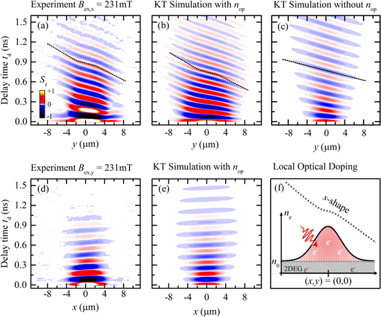
Figure 18. Experimental and simulated spatio-temporal maps in false-color representation, displaying the tilt of the CdTe PSH in external magnetic fields. (a-c) Measurement along the y-axis (a), one KT simulation takes a local modulation of α and β into account (b) whereas the other does not (c). (d-e) Measurement and KT simulation along the x-axis with nop analogous to (a) and (b. (f) Schematic injection of a Gaussian photo-carrier distribution in addition to the resident 2DEG in the QW, forming the origin of the saddle-point-like stripes seen in the measurements as black, dashed lines.
Download figure:
Standard image High-resolution imageFigure 18(c) shows a simulation based on kinetic theory. Generally, this simulation is in good agreement with the experiment shown on the opposite side of the figure since the increased tilt and the number of oscillating stripes are reproduced. However, upon closer inspection the attention is drawn to a phenomenological feature of the experiment missing in the simulation. This feature is the saddle-point-like appearance of the stripes in the experiment highlighted in the plot by a dotted line. While this behavior is striking along the y-axis, it is much weaker in the data along the x-axis. It is completely absent in the kinetic theory (KT) simulation as indicated by a straight, dashed line in the simulation panel. Generally, the feature is not predicted by the theoretical model which predicts a constant tilt based on spatially constant SO coupling. The observed saddle-point-like shape, on the other hand, points more at a slowing down of vy1 with electrons, propagating away from the origin at y = 0 μm. Taking into account the formulae in equation (50) such a spatial modulation of the stripe's slope can only arise from the α and β parameters being different in the center of the plot than at the edges, since all other entities in the theory are constants. Attempting to explain a locally disturbed SO coupling, it is reasonable to consider an influence of the photo-excitation process triggering the PSH formation. This excitation creates a non-equilibrium regime that affects the PSH if sufficiently many photo-carriers are involved.
Figure 18(f) illustrates a schematic of the spatial profile picture of the carrier density composed of a locally injected density nop and the resident 2DEG electrons with density n0. In case that nop and n0 are of similar size it is plausible that the SO coupling parameters are spatially modulated. Such a modulation takes place due to screening of the electric field in the case of α and a direct renormalization of the Fermi wave vector  that determines β3. Due to the multiple influences of the carrier density on the system, a direct quantification of the above introduced hypothesis turns out to be challenging. Therefore, measurements dependent on the excitation power are performed. The peak photo-injected carrier densities are in the range of (0.5 − 2.6)n0, i.e. comparable to n0 = 3.4 × 1011 cm−2. Figure 19(a) depicts five line scans taken under the same conditions, varying only the optical peak intensity. For a better comparison among the individual measurements and also to the results of the simulations, only the data for positive y-values is selected from the symmetric scans. Studying individual line scans for a fixed td = 750 ps enables the inspection of subtle features that are much harder to recognize in full spatio-temporal maps. The normalized experimental curves undergo a strong change of shape while the intensity is raised. An increased modulation depth together with a longer ranging spin precession length are visible in the experimental data where both trends are highlighted with arrows. From the experiment it is apparent that the higher the intensity is, the further away from the origin, the signal can still be detected. This finding suggests an increased diffusion which is confirmed by individual analysis of the full spatio-temporal map for each intensity (data not shown). In accordance to the inset in figure 19(d), a linear rise of Ds with increasing intensity is confirmed. Additionally, the same inset illustrates the estimated photo-carrier density in dependence on Iop, explaining the increased diffusion coefficient as follows. The Fermi energy depends directly on the electron density in the system and a locally elevated density will result in an increased Fermi energy and velocity which follow the same distribution. Moreover, the Fermi velocity is a determining part of the diffusion coefficient given by
  . However, the direct calculation of a general Ds is complicated by this spatial and temporal density modulation, the latter being caused by the recombination of 2DEG electrons with holes. While spatial modulation cannot be reasonably considered, the lifetime of electrons for similar structures is known to be comparable or shorter than the spin lifetime [74, 75]. For the present sample a lifetime of Tc ∼ 1 ns is obtained from transient reflectivity measurements (data not shown).

Figure 19. (a) Experimental line scans for varying optical intensities taken at td = 750 ps. (b-c) KT simulations of the experiment with changes of only nop (c) or only Ds (b) in accordance with the inset that relates both entities with the peak laser intensity. (d) KT simulation based on spatially modulated SO coupling parameters and diffusion coefficient that reproduces the qualitative trends of the experiment illustrated by grey arrows.
Download figure:
Standard image High-resolution imageIt has been shown in the previous section that a changed diffusion coefficient has a severe influence on the measured spin precession length  due to a faster or slower transition from a multi-mode Gaussian to the single-mode PSH. For this reason it is vital to review the possibility that the variation of the diffusion itself causes the differently shaped line scans observed in the experiment. Figure 19(b) displays KT simulations for the same parameter set as encountered in the experiment. A pronounced increase in the modulation depth can be achieved. However, the simultaneous variation of the spin precession length is not reproduced, resulting in a visible deviation of the simulation from the experiment. This leads to the conclusion that, indeed, the photo-carrier density plays an important role in the SO coupling process and an according model is required to verify this assumption. For a further validation a dynamic carrier density in space and time is modeled by the expression
that combines intrinsic and optical doping, with nop being the average initial photo-carrier density within the laser spot. The combination follows an approach that considers the diffusive broadening of the electron distribution as well as the temporal decay due to recombination and is schematically shown in figure 18(f). The expression in equation (51) enters directly into the calculation of the cubic Dresselhaus parameter as

It imposes a novel spatio-temporal dynamics to  . Beyond this influence, it is reasonable to incorporate a similar dependence into α. The Rashba parameter is indirectly affected as additional charges screen the internal electric field in the QW, entering into
  . An according model is based on the depolarization field
  created by a carrier density δ ne. The depolarization field is given by

where denotes the dielectric constant and ρ is a dimensionless parameter that depends on the shape of the QW and is not strongly affected by the carrier density itself. From this consideration the impact of optical doping can be incorporated into the Rashba coefficient according to

where α0 represents the as-grown Rashba parameter, formerly refered to as α. By now, the differential equation employed for kinetic theory simulations can be equipped with the new expressions for α and β3 and solved numerically. This yields the simulated curves in figure 19(c) where the optical density is chosen from the relation shown in the inset, matching the intensities used in the experiment. The obtained simulations reveal a strong tuning of the zero crossings for the signal whereas the distinct tuning of the modulation depth seen in the experiment is not reproduced. As a consequence, the local variation of the SO coupling alone can not be the origin of the s-shape. However, a combined approach, where an increase of the diffusion coefficient and of the optical density is considered, reproduces the observations. This combination leads to the set of simulated curves in figure 19(d). Now, these simulations show a remarkable agreement with the experiment as both the modulation strength and the shift in the precession length are qualitatively reassembled.
The agreement stands as a strong evidence for the assumed influence of optical doping on the PSH. This finding is strengthened by the proof that neither changes of Ds nor of nop alone can explain the experiment. Moreover, the same kinetic theory model is used to investigate the origin of the unexplained s-shape that motivated the idea of photo-carrier induced fine tuning. Figure 18 contains two false-color plots in panel (b) and (e) which depict KT simulations with density-dependent SO coupling parameters and the s-shape of stripes is now clearly recognizable. This visual comparison serves as an additional validation of the photo-injected carrier density as fine tuning knob for the PSH and finally explains the saddle-point-like behavior. There is no fundamental reason that a similar effect of photoexcited carriers as discussed above should not appear in the GaAs sample. However, GaAs has a smaller absorption and in the regime analyzed here the photocarrier density remains smaller than the density of the 2DEG. Therefore, we do not observe s-shape stripe pattern in GaAs.
6. Summary
The present review summarizes recent advances in the area of PSH physics. In particular we present a comprehensive analysis of operating conditions and system parameters, including the Fermi energy, the diffusion coefficient, electric and magnetic fields and the Rashba and Dresselhaus parameters themselves. On the one hand, we investigate the complex mutual dependences of these tuning knobs in the prototypical material GaAs. On the other hand, additional effects are discovered in the previously unstudied material CdTe where optical doping is identified as a novel tuning mechanism. A schematic overview about the most striking results compiled in this review is given in figure 20.

Figure 20. Overview of manipulation schemes studied in the present review. (a) Application of back-gate voltage allows for tuning of α and β3. (b) By applying voltages to the Hall bar structure, the spins can be translated along the QW, leading to a strong variation of (α + β ). (c) Optical doping of the CdTe sample results in a local gradient of the Rashba and cubic Dresselhaus parameters, manifesting as s-like shaped polarization stripes in the spatio-temporal maps with applied external magnetic field.
Download figure:
Standard image High-resolution image
In summary, the SO coupling parameters α and β substantially change with the electric field applied to the 2DEG within the GaAs QW via a back-gate. By studying the spatial precession lengths λ0,x and λ0,y along the ![$[1\bar{1}0]$](https://content.cld.iop.org/journals/0268-1242/34/9/093002/revision2/sstab3158ieqn229.gif) and [110] directions the sum, difference and individual values of α and β are extracted (see section 5.2.3). Moreover, the Dresselhaus parameter can be separated into a linear and cubic contribution. All the extracted parameters are given in figure 20(a), where the effect of an increasing gate field on the SO coupling is depicted. A pronounced decrease of the Rashba parameter with increasing UBG confirms the direct relation of α with the external electric field
and [110] directions the sum, difference and individual values of α and β are extracted (see section 5.2.3). Moreover, the Dresselhaus parameter can be separated into a linear and cubic contribution. All the extracted parameters are given in figure 20(a), where the effect of an increasing gate field on the SO coupling is depicted. A pronounced decrease of the Rashba parameter with increasing UBG confirms the direct relation of α with the external electric field  across the heterostructure. A nearly constant value for β1 is found in agreement with the theory model whereas the increase of β3 is attributed to a change of the electron density via UBG. As a result of the simultaneous variation of density and the α/β ratio, the spin lifetime shows a peak-like dependence on UBG. In general, the back-gate allows for direct modification of the Rashba SO coupling, making it an advantageous tuning knob for spintronics. In contrast, the diffusion coefficient
  is not significantly altered by UBG. This is explained by a canceling of simultaneous changes in EF and the scattering time τee with increasing electron density.
The spatio-temporal analysis of the spin polarization as a function of in-plane electric and magnetic fields shows manifold modifications of the PSH pattern. Until now, the negligible precession of spins traveling perpendicular to the spin helix pattern prevented the extraction of the difference (−α + β). By tilting the spatio-temporal evolution of the spin pattern with magnetic fields applied along the ![$[1\bar{1}0]$](https://content.cld.iop.org/journals/0268-1242/34/9/093002/revision2/sstab3158ieqn232.gif) and [110] this drawback has been removed. Accordingly, the individual Rashba and Dresselhaus parameters can be precisely extracted (see section 5.2.1). Despite the direct interaction of effective and external magnetic fields, a dependence of the SO coupling on the applied field strength was not observed. However, a strong effect on the SO parameters is found for anisotropic spin transport where in-plane electric fields reveal a tunability of the spin precession length λ0,y. Figure 20(b) depicts the related increase of (α + β) with field strength and a similar trend is found for λ0,x and (−α + β) (see figure 16). This review also presents an in-depth analysis of spin drift perpendicular to the spin helix pattern. Such fields reveal oscillations along
and [110] this drawback has been removed. Accordingly, the individual Rashba and Dresselhaus parameters can be precisely extracted (see section 5.2.1). Despite the direct interaction of effective and external magnetic fields, a dependence of the SO coupling on the applied field strength was not observed. However, a strong effect on the SO parameters is found for anisotropic spin transport where in-plane electric fields reveal a tunability of the spin precession length λ0,y. Figure 20(b) depicts the related increase of (α + β) with field strength and a similar trend is found for λ0,x and (−α + β) (see figure 16). This review also presents an in-depth analysis of spin drift perpendicular to the spin helix pattern. Such fields reveal oscillations along ![$[1\bar{1}0]$](https://content.cld.iop.org/journals/0268-1242/34/9/093002/revision2/sstab3158ieqn233.gif) unseen in purely diffusive experiments, allowing for the extraction of (−α + β) from the spin precession length λ0,x. Moreover, oscillations along the x-axis enable the extraction of β3 from temporal precession which is induced by external drift fields, having been seen previously along the y-axis only.
unseen in purely diffusive experiments, allowing for the extraction of (−α + β) from the spin precession length λ0,x. Moreover, oscillations along the x-axis enable the extraction of β3 from temporal precession which is induced by external drift fields, having been seen previously along the y-axis only.
Section 5.3 reports the experimental demonstration of the PSH formation in a 2DEG that is hosted in a II-VI material, namely a high mobility CdTe QW sample. Confirming the universality of the PSH, the SO coupling is found to be close to a perfectly balanced regime, featuring a ratio of α/β = 1.3. The characteristic PSH evolution is well comparable to the behavior in GaAs and allows for the extraction of a diffusion coefficient and the Rashba and Dresselhaus parameters, employing the already developed methods. It is found that a locally injected distribution of photo-carriers affects the SO coupling parameter and the diffusion coefficient. This relation is modeled with a Gaussian distribution of electrons in space that translates into a gradient in the Rashba and cubic Dresselhaus parameters. While the change in α is explained by screening effects of the internal electric fields, β3 is changed by a local elevation of the Fermi energy. This considerations arise from a s-like distortion of the polarization stripes in spatio-temporal maps with applied external magnetic field as displayed in figure 20(c). In order to validate the proposed model, the spin precession is studied in dependence on the photo-carrier density. Subsequently, the results are successfully compared with kinetic theory simulations that incorporate local perturbations due to photo-carriers, making α and β dependent on time and space. The finding of a precession length that can be modified all-optical by the laser intensity is an important key for a control of SO coupling in semiconductor nanostructures.
Acknowledgments
The experimental work in this review heavily relies on the supply of high-quality semiconductor heterostructures with high-mobility 2DEGs. GaAs-based heterostructures have been provided by J N Moore and G Yusa from the Department of Physics and the Center for Spintronics Research Network at Tohoku University in Sendai, Japan, as well as by T Mano and T Noda from the National Institute for Materials Science in Tsukuba, Japan. CdTe-based heterostructures have been fabricated by G Karczewski and T Wojtowicz from the Institute of Physics of the Polisch Academy of Science and the International Research Center MagTop in Warsaw, Poland. We thank T Tischler for assistance in early measurements on the CdTe samples and K. Schiller for assistance with the MC simulations.
We acknowledge financial support by the International Collaborative Research Center ICRC TRR 160 'Coherent manipulation of interacting spin excitations in tailored semiconductors' based in Dortmund, Germany, and St. Petersburg, Russia. It is funded by the DFG under the project number 249492093, subproject B3, and by the RFBR, project No. 19-52-12038. AVP also acknowledges the support by the Foundation for the Advancement of Theoretical Physics and Mathematics 'BASIS' and the Russian President Grant No. MK-599.2019.2.