

Abstract
Can the laws of physics be unified? One of the most puzzling challenges is to reconcile physics and chemistry, where molecular physics meets condensed-matter physics, resulting from the dynamic fluctuation and scaling effect of glassy matter at the glass transition temperature. The pioneer of condensed-matter physics, Nobel Prize-winning physicist Philip Warren Anderson referred to this gap as the deepest and most interesting unsolved problem in condensed-matter physics in 1995. In 2005, Science, in its 125th anniversary publication, highlighted that the question of 'what is the nature of glassy state?' was one of the greatest scientific conundrums for the next quarter century. However, the nature of the glassy state and its connection to the glass transition have not been fully understood owing to the interdisciplinary complexity of physics and chemistry, governed by physical laws at the condensed-matter and molecular scales, respectively. Therefore, the study of glass transition is essential to explore the working principles of the scaling effects and dynamic fluctuations in glassy matter and to further reconcile the interdisciplinary complexity of physics and chemistry. Initially, this paper proposes a thermodynamic order-to-disorder free-energy equation for microphase separation to formulate the dynamic equilibria and fluctuations, which originate from the interplay of the phase and microphase separations during glass transition. Then, the Adam–Gibbs domain model is employed to explore the cooperative dynamics and molecular entanglement in glassy matter. It relies on the concept of transition probability in pairing, where each domain contains e + 1 segments, in which approximately 3.718 segments cooperatively relax in a domain at the glass transition temperature. This model enables the theoretical modeling and validation of a previously unverified statement, suggesting that 50–100 individual monomers would relax synchronously at glass transition temperature. Finally, the constant free-volume fraction of 2.48% is phenomenologically obtained to achieve a condensed constant (C) of C= 0.12(1−γ) = 1.501 × 10⁻¹¹ J·mol−1·K−1, where γ represents the superposition factor of free volume and is characterised using the cumulative Poisson distribution function, at the condensed-matter scale, analogous to the Boltzmann constant (kB) and gas constant (R).
Export citation and abstract BibTeX RIS

Original content from this work may be used under the terms of the Creative Commons Attribution 3.0 license. Any further distribution of this work must maintain attribution to the author(s) and the title of the work, journal citation and DOI.
Recommended by Dr Mark Geoghegan
1. Introduction
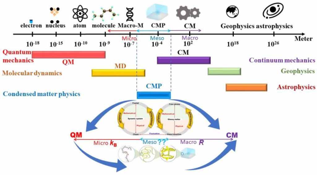
Figure 1 shows a unified perspective on a selection of length scale in physics, ranging from the electron at 10−18 m, atomic nucleus at 10−15 m, and atom at 10−10 m, to molecule at 10−9 m, macromolecule at 10−7 m, condensed-matter at 10−4 m, classical mechanics at 102 m, geophysics at 108 m, and astrophysics at 1026 m [1]. Notably, understanding these length scales in physical systems has become essential to create predictive simulations across multiple length scales and to pursue the answer for unifying physical laws [1–6]. Therefore, it is important to get an idea of how big differences in different length scales [2, 3, 5]. For instance, the Bohr model of single-electron atoms resembles planetary orbits but exhibits scaling differences [7], signifying the scaling effect between atomic physics and geophysics [8]. Furthermore, the scaling effects in condensed matter of dynamic glass transition may originate from the interplay of inter-chain phase and intra-chain microphase separations.
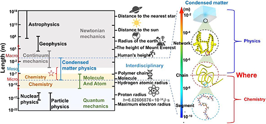
Figure 1. Length scale for dynamic glass transition, where the dynamic fluctuation is originated from the interdisciplinary of condensed-matter physics and chemistry (molecular physics).
Download figure:
Standard image High-resolution imageHere, the scaling effects of two distinct length scales are essential for reconciling the interdisciplinary laws, as shown in figure 2. However, studies on scaling effects are challenging because they originate from different areas of physics [9, 10]. Dynamic fluctuations can occur suddenly [2], resulting in a non-equilibrium and discontinuous but self-consistent scaling effect. Note that there is a scaling effect for glassy matter undergoing a dynamic glass transition [3, 5], at the two condensed-matter and molecular length scales. As molecular physics has been recognised as a part of chemistry, it is possible to achieve the scaling effect of the dynamic glass transition in glassy matter based on the reconciliation of condensed-matter physics and molecular physics (chemistry).
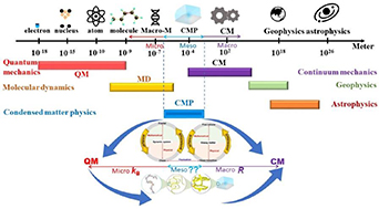
Figure 2. Scaling effect of condensed-matter physics, of which a condensed constant is expected to connect to the Boltzmann constant (kB) and gas constant (R).
Download figure:
Standard image High-resolution imageThe nature of glassy state is probably one of the most intricate challenges in condensed-matter physics [11]. Even in crystalline matter, achieving 100% crystallinity is often elusive, leading to the presence of amorphous matter. Furthermore, the glass transition presents complex dynamics that can be classified into various phase transition models. In 2005, the question 'what is the nature of glassy state?' was suggested as one of the greatest scientific conundrums over the next quarter-century for Science's 125th anniversary [12]. Studies on the nature of glassy matter have been ongoing for several decades, because of its fundamental significance and broad implication for condensed-matter physics [13–17]. There are numerous motivations for studying glassy matter, and the reasons this research field received increasing attentions have been explained by numerous enumerations [18]. In condensed-matter physics, the nature of glassy matter and its connection to glass transition are some of the most essential and fascinating topics. This is because much of condensed matter originates from its glassy state, resulting in an inseparable connection between dynamic fluctuation and glass transition. However, theoretical efforts remain at the phenomenological and empirical levels, with the fundamental scientific explanation yet to be understood [19].
Glassy matter exists in a non-equilibrium, amorphous, and condensed state, which appears solid within a short time scale, but gradually transitioning toward a liquid state, while avoiding crystallisation [20]. After decades of research, glass transition in glassy matter, which is considered a paradigmatic model of dynamic heterogeneity [21], remains a challenge in condensed-matter physics. According to previous studies on glassy matter and its connection to glass transition, there are two open issues, Kauzmann's paradox and the jamming phenomenon, necessitating the development of a novel theoretical framework for understanding. In the last decades, three well-known models of glass transition have been developed: vibration-entropy, dynamic heterogeneity and melting-entropy models.
In 2010, Pedersen et al proposed a vibration-entropy model using repulsive inverse-power-law potentials to reproduce the structure, dynamics, and isochoric heat capacity of glassy matter [22]. In 2014, Wang and Xu proposed a vibration-entropy model to relate the density and glass transition temperature of Lennard–Jones and Weeks–Chandler–Andersen systems, which can be predicted from the properties of zero-temperature glass [23]. Dell and Schweizer formulated a model in terms of repulsive and attractive forces, to predict the apparent Arrhenius behavior and density-temperature scaling in glassy matter undergoing slow dynamics [24]. In 2020, Chattoraj and Ciamarra demonstrated that the nonperturbative dynamic effects of attractive forces were equivalent to the activation energy at the glass transition temperature, resulting in consistent dynamic properties for various types of glassy matter, including metals, polymers, or colloids, when subjected to the same level of attractive forces [25]. Furthermore, Mahajan and Ciamarra unified the description of vibrational anomalies using elastic disorders and localised defects in glassy matter [26].
The α-relaxation typically involves large and cooperative rearrangements during the glass transition, while the β-relaxation pertains to smaller-scale structural rearrangements within the glassy state. It is expected that there is a strong relationship between α-relaxation and β-relaxation, resulting from the dynamic heterogeneity in glassy matter [27–30]. In 2011, Liu et al provided the first experimental evidence of nanoscale viscoelastic heterogeneity in metallic glasses characterised by dynamic force microscopy. This finding bridges the gap between atomic models and macroscopic glass properties [27]. In 2011, Keys et al employed trajectory space to study the structure, statistics, and dynamics of the excitations responsible for structural relaxation [28]. This study was helpful in developing a string model based on the Adam–Gibbs (AG) theory, and in exploring the effect of string-like motion on glass transition [29]. In 2022, Li et al demonstrated that the relaxation dynamics of supercooled liquids correlated well with the plastic length scale of particles. They found that the average plastic length scale controlled the super-Arrhenius relaxation time, while the local elastic response only correlated the dynamics with the vibrational timescale [30].
The melting-entropy model is one of the most popular approaches for characterising glass transitions in glassy matter. In 2013, Zaccone and Terentjev explored the working principle of the melting transition of amorphous (disordered) solids in terms of the lattice energy. This offers a new opportunity to relate dynamic glass transitions to melting transitions [31]. In 2023, Lunkenheimer et al introduced the Lindemann criterion to formulate a constitutive relationship between the glass transition temperature and thermal expansion using the melting transition temperature [32]. Furthermore, Ren et al found that there is a strong dependence of melting viscosity on melting entropy, which governs glass formability. An apparent link between melting point and glass formation has been explored and discussed [33].
In this study, a thermodynamic order-to-disorder free-energy equation for microphase separation is proposed based on the transition probability. This equation formulates the dynamic equilibria for glass transition, where fluctuations originate from the interplay of the phase and microphase separations at two distinct scales: the condensed and molecular levels. This approach is used to reconcile physics and chemistry at both the condensed-matter and molecular scales. Moreover, the AG model has been introduced to explore the dynamic cooperativity of a constant domain size z= e + 1 at the glass transition based on the principle of maximum entropy (or minimum entropy production) and transition probability in pairing, and verify the previously published finding stating that 50–100 monomers relax synchronously at glass transition. Additionally, the connection between glass transition and free volume, which originates from the Einstein mass-energy equilibrium (E= Mc2, where E is the cohesive energy, M is the mass, and c is the velocity of light) [34], has been identified as a constitutive relationship between dynamic chaos and fractals. Subsequently, a complex fractal function was introduced to predict the trial guide of the free volume. This function follows the self-consistency and power laws, where the scaling effect is a result of differences in the fractal dimensions between the molecular chain and condensed matter. A free-volume equilibrium was developed using dynamic separation of the dense and dilute phases. This equilibrium verifies that glass transition occurs at a constant fraction of free volume of 2.48%, which is then used to achieve a condensed constant of C= 0.12(1−γ) = 1.501 × 10⁻¹¹ J·mol−1·K−1 (where γ is the superposition factor of free volume) at the condensed-matter scale, analogous to the Boltzmann and gas constants. Finally, this study provides a fundamental framework to understand the nature of glassy matter and formulate the dynamic equilibrium of glass transition. Dynamic fluctuations originate from the interplay of interdisciplinary complexity at two condensed and molecular scales, where physics meets chemistry.
2. Connection of glass transition to the transition probability
2.1. Dynamic equilibrium of glass transition
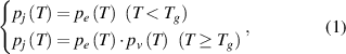
The Eyring equation was previously combined with the Williams–Landel–Ferry equation to characterise the thermodynamics of glass transition in amorphous polymer [35]. In the glassy state, the relaxation of molecular chains requires sufficient activation energy to overcome the energy barriers. Conversely, in the rubbery state, molecular chains require free volume to be available in order to jump, as no further energy barrier exists to constrain their dynamic relaxations [36]. Therefore, the transition probability ( ) of a molecular chain relaxing around
  can be written simply as:
where  is the transition probability of a molecular chain to obtain sufficient activation energy to overcome the energy barrier and
  is the transition probability to obtain sufficient free volume available to jump.
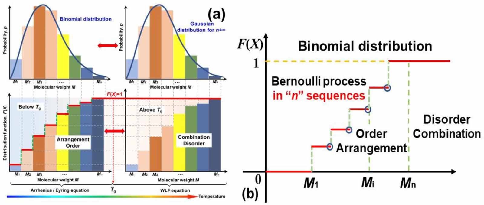
Based on a binomial distribution (Bernoulli distribution) with parameters n and p, the discrete distribution is a sequence of n independent statistics. Here, a single step is called a Bernoulli trial and a sequence of steps forms a Bernoulli process. Therefore, the transition probability of the molecular chains relaxing is governed by the mathematical arrangement of the Bernoulli process below Tg
, where the random variable (p(X)) is 1 or 0 depending on whether the molecular chain relaxes or not. As shown in figure 3(a), the constitutive relationship between the distribution function (F(Mi
)) and the molecular weight (Mi
) was plotted based on the transition probability of the Bernoulli distribution for glassy matter. Therefore, below Tg
, glassy matter presents a transition probability of the mathematical arrangement, and molecular chains do not relax unless sufficient activation energy is obtained [35]. Consequently, above Tg
, there is a transition probability of a combination, where the molecular chains have acquired sufficient activation energies for relaxation. It is well known that physical order and disorder can be represented by mathematical arrangement and combination, respectively [37]. Therefore, based on the probability of Bernoulli distribution function  , where Mi
is the molecular weight, the glass transition of glassy matter is a physical order-to-disorder or mathematical arrangement-to-combination problem, as shown in figure 3(b).
, where Mi
is the molecular weight, the glass transition of glassy matter is a physical order-to-disorder or mathematical arrangement-to-combination problem, as shown in figure 3(b).
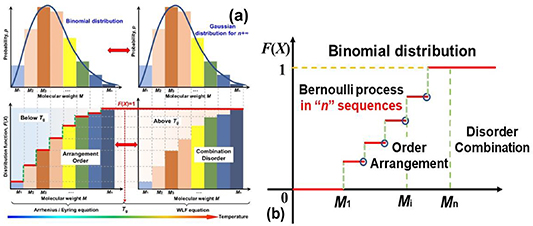
Figure 3. (a) Bernoulli distribution of molecular weight of glassy matter, which presents the order and arrangement relaxation below Tg , as well as the disorder and combination relaxation above Tg . (b) Physical order-to-disorder for the glass transition of glassy matter.
Download figure:
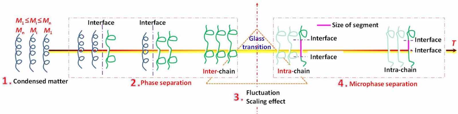
Standard image High-resolution imageAs shown in figure 4, the relaxation behavior of glassy matter is derived from the molecular chain below Tg , whereas it originates from the molecular segment above Tg . Therefore, glass transition has been identified as the temperature at which segmental relaxation in a molecular chain starts [38, 39]. The relaxation motion of a molecular chain must overcome the intermolecular constraints of other chains in their condensed states, and is governed by the thermodynamics of phase separation [40, 41]. Meanwhile, the relaxation motion of a segment has to overcome the intramolecular constraints of other segments in a molecular chain and is governed by the thermodynamics of microphase separation [40, 41].

Figure 4. Schematic illustrations of molecular chains undergoing phase and microphase separations below and above Tg , respectively, where the glass transition is originated from the starting temperature point of relaxation motion for the segment.
Download figure:
Standard image High-resolution imageTherefore, the dynamic equilibrium of glass transition is derived from the ordered ( ) and disordered (
 ) free energies of the segments undergoing microphase separation in a molecular chain. According to the thermodynamics of microphase separation, the ordered (
 ) free energy is expressed as follows [40, 41],
where  is the interfacial tension [41],
  is the interfacial area [40],
  is the interaction parameter between two microphases [38, 41],
  is the interfacial thickness [42], b is the segment length, R is the gas constant,
  , is the number of monomers in a dynamic segmental unit, where
  and
and  are the volumes of segment and monomer, respectively [41]. If the lowest ordered free energy is achieved, that is,
  ,
,  , and
, and  are the periodic interfacial thickness [40, 41], the ordered free-energy function can be expressed as follows,

The disordered free energy of the segment is employed as follows [40, 41],

where  and
and  are the volume fractions of the ordered and disordered microphases in the molecular chain, respectively. At Tg
, it is assumed that
are the volume fractions of the ordered and disordered microphases in the molecular chain, respectively. At Tg
, it is assumed that  , according to the Flory–Huggins (FH) solution theory, that is, the volume fractions of the two phases are equal at the critical point [40–42].
Combining equations (3) and (4), the thermodynamic equilibrium of microphase separation can be obtained as,

Here,  is also used to characterize the interaction parameter between the order and disorder microphases. If one supposes that there is a strong interaction between these molecular segments, then, for example, a value of
  , where the degree of polymerization for a microphase is incorporated from 3.718 dynamic segmental units at Tg
[43, 44] based on the AG model [45], would mean that N≈ 19.5. Equivalently, the basic segment containing N≈ 19.5 monomers undergoes microphase separation at Tg
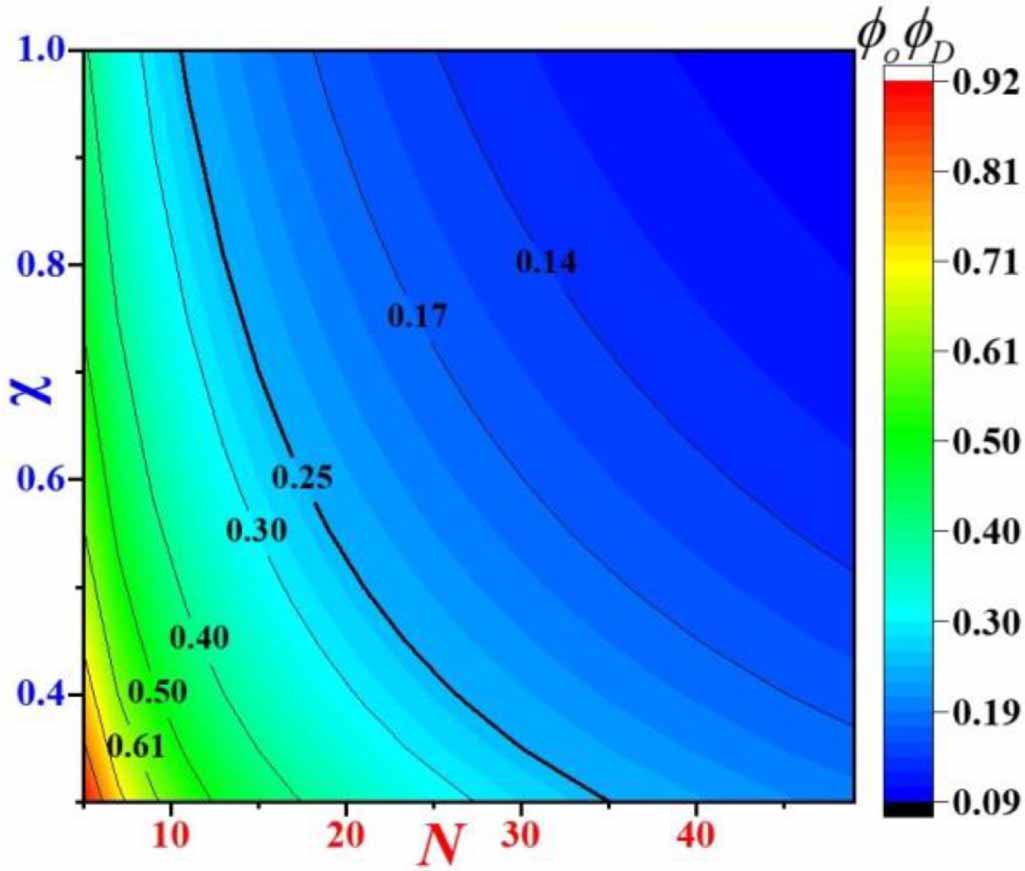
. Furthermore, figure 5 plots the constitutive relationship of the interaction parameter (
, where the degree of polymerization for a microphase is incorporated from 3.718 dynamic segmental units at Tg
[43, 44] based on the AG model [45], would mean that N≈ 19.5. Equivalently, the basic segment containing N≈ 19.5 monomers undergoes microphase separation at Tg
. Furthermore, figure 5 plots the constitutive relationship of the interaction parameter ( ) as a function of number of monomers (N) in a dynamic segmental unit. It becomes evident that the number of monomers (N, where we assume N= NO
= ND
) in a dynamic segmental unit is gradually increased with a decrease in the interaction parameter (
) as a function of number of monomers (N) in a dynamic segmental unit. It becomes evident that the number of monomers (N, where we assume N= NO
= ND
) in a dynamic segmental unit is gradually increased with a decrease in the interaction parameter ( ).
).

Figure 5. Cloud chart of interaction parameter ( ) and number of monomers in the dynamic segmental unit (N) as functions of the volume fractions of order and disorder microphases (
 ) in the molecular chain.
Download figure:
Standard image High-resolution image2.2. Dynamic cooperativity and molecular entanglement at glass transition
Similar to quantum entanglement in quantum mechanics, molecular entanglement exists and has been identified using the dynamic cooperativity of glassy matter undergoing a glass transition [45]. This is because the relaxation of each segment cannot be individually characterised and is completely enveloped by the dynamic cooperativity of all the segments in the AG domain system. Therefore, the molecular entanglement originates from the dynamic cooperativity in condensed matter. Owing to this molecular entanglement, the configurational entropy of a segment is aligned to that of the domain in mathematics, whereas the glass transition of glassy matter is derived from the AG domain in physics rather than a segment within it.
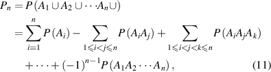
The dynamic equilibrium of glass transition was formulated based on the thermodynamic microphase separation and order-to-disorder free-energy functions. Dynamic cooperativity or molecular entanglement has not yet been formulated for glass transition in glassy matter. The AG domain size model provides an effective approach for studying the dynamic cooperativity of glassy matter [45]. The cooperatively rearranging region (CRR) has been developed to explain the cooperatively dynamic relaxation of glassy matter [46, 47], where the number of segments in a CRR domain is defined as the domain size (z). All these segments relax cooperatively and simultaneously to overcome their potential energy barriers, which restrict relaxation and rearrangement. All segments relaxed synchronously in a domain, and each segment had the same dynamic characteristics.
For 1 mol of segments involved in cooperative relaxation, the configurational entropy ( ) can be written as [48],

where  is the number of domains and
  = 1.38 × 10⁻²³ J K−1 is the Boltzmann constant. Additionally, Ω is the configurational number of the dynamic segment, which relaxes cooperatively and synchronously in a domain [46–48].
The relationship between domain size (z) and number of domains ( ) for 1 mol of basic dynamic segments can be obtained as follows [49],

where  = 6.02 × 10²³ is the Avogadro's number.
According to the AG model, the activation energy of a domain is determined by its size (z). With increasing temperature, the domain size (z) decreases, whereas the configurational entropy increases accordingly [34, 49]. By substituting equations (6) into (7), the constitutive relationship between the domain size (z) and configurational entropy ( ) can be expressed as follows [49, 50],

Here,  is defined as the maximum value of the configurational entropy of 1 mol of dynamic segments, whose relaxation is not mutually restricted by others at the temperature
  , resulting in z = 1 [34]. Therefore,
  can be written as follows,

By substituting equation (9) into (8), the domain size (z) can be obtained as,
Based on the AG model, the configurational entropy ( ) can be expressed by the domain size in the temperature range from
  to
to  , where
  is defined as the temperature at which all the conformers are integrated into a single domain and the configurational entropy is equal to zero, leading to z = ∞ [34, 44, 51]. However, the z =1 at
  at which the cooperative relaxation of the conformers becomes independent. In the temperature range from
  to
to  , there are infinite values for domain size (z), where z is ranged from 1 ⩽ z < +∞. To identify cooperative relaxation using configurational entropy (
 ), the transition probability of the pairing problem is employed to characterise the domain size (z). In other words, the transition probability should meet the requirement of at least one dynamic segment that starts relaxation at
  , where the segments must be paired with their corresponding molecular chains.
If there are n (1 ⩽ n< +∞) molecular chains, there are n corresponding dynamic segments that undergo relaxation within these chains at  . For a discrete probability distribution, a binomial (or Bernoulli) distribution was used to characterise the probability (p) for n independent in statistics. Based on the two parameters of the binomial distribution, namely, n, representing the number of trials, and p, signifying the event or success probability, the random variable (p) is 1 or 0 depending on whether the event occurs. However, with an increase in the n independences, that is, n → +∞, and the infinitesimal probability, p → 0, the Poisson probability distribution, in which the events occur independently, is then employed to describe the discrete probability of the number of events occurring in a given time period.
There are two requirements for the transition probability at  , (1) at least one dynamic segment relaxes, and (2) the relaxed segment is paired with its molecular chain. Based on the pairing issue of the transition probability, the transition probability (
 ) can be expressed as
where  is the transition probability for the ith segment in its molecular chain starting to relax,
 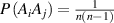 (
( ) is the transition probability for the ith and jth segments in their molecular chains that start to relax,
 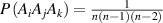 (
( ) is the transition probability for the ith, jth and kth segments in their molecular chains that start to relax, and
  .
.
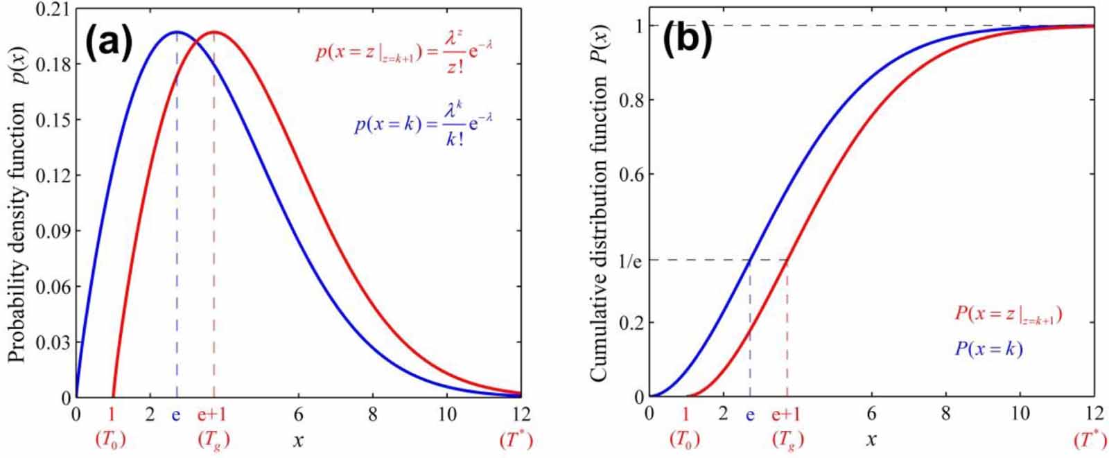
Thus, the transition probability ( ) can be obtained as,
where e = 2.71828 is the Eulerian constant.
Based on equation (12), the transition probability ( ) for the case where at least one basic segment starts to relax in pairs with its corresponding molecular chain is
 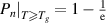 . The transition probability is
  in the temperature range of
  , resulting in the configurational entropy (
 ) of
) of  and
and  [52, 53]. Furthermore, the domain size range is 1 ⩽ z < +∞, resulting in a shift in the domain size to z(Tg
) = e + 1, as shown in figure 6, where the curves of Poisson probability density function and its cumulative Poisson distribution function are plotted to characterise the glass transition. As is well known, the domain size (z) is determined by the configurational entropy (
[52, 53]. Furthermore, the domain size range is 1 ⩽ z < +∞, resulting in a shift in the domain size to z(Tg
) = e + 1, as shown in figure 6, where the curves of Poisson probability density function and its cumulative Poisson distribution function are plotted to characterise the glass transition. As is well known, the domain size (z) is determined by the configurational entropy ( ) and configurational number (Ω), which is equal to the domain size (z) at Tg
[44, 51], that is, Ω(Tg
) = z(Tg
) = e + 1 ≈ 3.718. Subsequently, the configurational entropy per mole of monomer is obtained as
) and configurational number (Ω), which is equal to the domain size (z) at Tg
[44, 51], that is, Ω(Tg
) = z(Tg
) = e + 1 ≈ 3.718. Subsequently, the configurational entropy per mole of monomer is obtained as  , leading to the configurational entropy per mole of domain
  ≈ (2.936) J kmol−1, which is in good agreement with the Wunderlich's and Chang's 'universal' value of
  = (2.9) J kmol−1 [54, 55]. Based on the transition probability theory,
  is a mathematical expectation, which is a numerical characteristics of the probability distribution of temperature ranging from
  to
to  .
.
Figure 6. Analytical curves of Poisson distribution functions. (a) For probability density of Poisson distribution ( ) as functions of domain size and temperature. (b) For cumulative Poisson distribution (
 ) as functions of domain size and temperature.
Download figure:
Standard image High-resolution imageAccording to equation (5), it is found that a dynamic segment contains  ≈ 19.5 monomers at Tg
, when
≈ 19.5 monomers at Tg
, when  = 0.538. Additionally, there are z(Tg
) = e + 1 ≈ 3.718 segments in a domain to relax due to the dynamic cooperativity and molecular entanglement. Therefore, there are
= 0.538. Additionally, there are z(Tg
) = e + 1 ≈ 3.718 segments in a domain to relax due to the dynamic cooperativity and molecular entanglement. Therefore, there are  ≈ 72 monomers to relax synchronously at Tg
. This result validates the assertion that 50–100 monomers in a molecular chain relax synchronously at the Tg
as confirmed by the newly proposed models.
≈ 72 monomers to relax synchronously at Tg
. This result validates the assertion that 50–100 monomers in a molecular chain relax synchronously at the Tg
as confirmed by the newly proposed models.
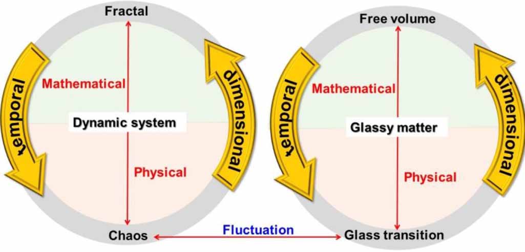
3. Time-space correlation between glass transition and free volume
Based on chaos theory, glassy matter is classified as a dynamically chaotic system that is always governed by deterministic laws and is highly sensitive to initial conditions. Glass transition is the dynamic fluctuation of glassy matter, in which the free volume provides dimensional space for relaxation. Therefore, the connection between the glass transition and free volume is governed by the constitutive relationship between dynamic chaos and mathematical fractals, that is, the glass transition is a temporal chaos of the free volume, whereas it is a dimensional fractal of the glass transition, as shown in figure 7.

Figure 7. Connection of glassy matter to the dynamic chaos system, in which the constitutive relationship between dynamic chaos and mathematic fractal is analogous to that between the glass transition and free volume.
Download figure:
Standard image High-resolution imageStudies of the glass transition of amorphous polymer, one of the most popular types of glassy matter, have been ongoing for decades since Flory and Fox formulated the free-volume theory. This theory suggests that the thermal expansion of glassy matter involves expansion of the free volume and occupied volume, which are occupied by voids and molecules, respectively [56–58]. Eyring correlated the glass transition with the activation energy [59]. Doolittle and Cohen–Turnbull introduced the concept of free volume and related it to the viscosity and diffusivity parameters to predict the glass transition of glassy matter [60–62]. Fujita was the first researcher to relate free volume to molecule diffusion in glassy matter [63, 64]. From this perspective, the connection between free volume and glass transition was well documented by White and Lipson [36].
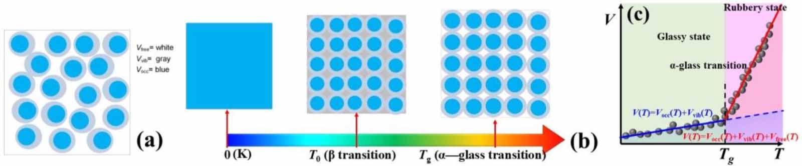
Inspired by this work, we used a stylised depiction of the various contributions to the total volume, with a guide to the notation listed below the diagram, as shown in figure 8(a). V is the total volume, the white region of Vfree is the free volume, the grey region of Vvib is the free volume for vibrational motion, and the blue region of Vocc is the occupied volume by the molecular chains. The temperature-dependent volume of glassy matter is presented in figure 8(b). At 0 K, the total volume of the glassy matter is completely occupied by the molecular chains, and there is no free volume for relaxation and vibrational motion, that is, V= Vocc. At T0, the total volume of the glassy matter is composed of the occupied volume (Vocc) and free volume (Vvib) of the molecular chains and their vibrational motions, respectively, that is, V= Vocc + Vvib. At Tg , the total volume of glassy matter is composed of three parts, the volume occupied by the molecular chains (Vocc) and two types of free volumes for relaxation and vibrational motion (Vvib + Vfree), thus, V= Vocc + Vvib + Vfree, resulting in a dynamic fluctuation of the total volume at Tg , as shown in figure 8(c).
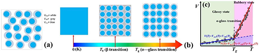
Figure 8. Diagram of different types of occupied volume and free volume in a glassy matter. Blue regions (Vocc) represent the volume occupied by the molecules. Grey regions are the free volume (Vvib) for the vibrational motion of segments, while they also play an essential role for the delta transition (δ transition) of monomer. White regions (Vfree) are the free volume available to the segments undergoing glass transition (α transition). (a) Free volume in glassy matter. (b) Temperature-dependent change in volume. (c) Dynamic fluctuation of volume function with respect to temperature at the glass transition temperature.
Download figure:
Standard image High-resolution imageAll these studies reported that the glass transition occurs at a specific free volume in glassy matter. However, research on the connection between the free volume and glass transition remains at the phenomenological model-building stages. Physical insights into the nature of free volume and its connection to glass transition remain perplexed.
3.1. Physical insight into free volume
The dynamic glass transition can be understood through the Flory–Fox free-volume theory, which considers the free volume as the internal space available for the mobility freedom of dynamic segment units [36, 57, 58, 60]. However, direct observation and examination of the free volume have not yet been achieved, and physical insight for the free volume remains at the phenomenological stage and is not fully understood [36]. Conventionally, the free volume has been consistently treated as a phenomenological and empirically determined parameter in previous models [36, 57, 58, 60].
According to the thermodynamics of phase and microphase separations, the free volume originates from the disassociation of cohesive energy and is governed by the Einstein mass-energy equilibrium [34]. Below Tg , the relaxation motion of the molecular chain results from the disassociation of the intermolecular cohesion (van der Waals forces) and is governed by the thermodynamics of phase separation. In contrast, the relaxation motion of a segmental unit in a molecular chain is derived from the disassociation of intramolecular cohesion (covalent forces) and is governed by the thermodynamics of microphase separation above Tg . At Tg , glassy matter undergoes an isometric transition [57] and an interplay of fluctuations in the phase and microphase separations, which are determined by intermolecular and intramolecular cohesions, respectively. Both intermolecular and intramolecular cohesions are governed by the Einstein mass-energy equilibrium, but with different constants. The dynamic fluctuation of glass transition in glassy matter results from differences in the disassociation of intermolecular and intramolecular cohesions at the condensed and molecular scales, respectively, resulting in a volumetric scaling effect. Therefore, there are two explicitly different constants in the Einstein mass-energy equilibrium used to describe intermolecular and intramolecular cohesion as functions of volume for glassy matter below and above Tg , respectively.
When segments are chemically crosslinked to form a molecular chain, the volume of the chain is smaller than the sum of the volumes of individual segments [65]. When the molecular chains are packed together to form a condensed matter, the volume is smaller than the sum of the volumes of the individual chains [65]. The increase in volume results from a decrease in cohesive energy [65]. The corrected values for the volumes and cohesive energies can be derived from the Einstein mass-energy equilibrium and expressed as follows [49],
where  and
and  are the correction factors introduced by Kanig for glassy matter below and above Tg
, respectively [66]. The subscripts 1 and 2 denote the initial and final states, respectively.
are the correction factors introduced by Kanig for glassy matter below and above Tg
, respectively [66]. The subscripts 1 and 2 denote the initial and final states, respectively.
Furthermore, the Einstein mass-energy equilibrium [34] is employed to construct the relationship between the mass and free volume for the cohesive energy as follows,
Based on equation (14), there is an inversely proportional relationship between the cohesive energy and volume. According to the AG model [34, 49], the domain size (z) is been employed to displace the mass, that is,  , leading to the following expressions,
Therefore, the change in volume is determined by the cohesive energy and is governed by the Einstein mass-energy equilibrium. The cohesive energies result from the intermolecular cohesive energy of the condensed chains and the intramolecular cohesive energy of the segmental units in a single chain. These energies resulted from the explicitly different constants in equation (15) below and above Tg .
3.2. Fractal perspective on free volume and its connection to scaling rule
Based on the chaos and fractal theory, glass transition is a dynamic fluctuation of glassy matter. During this fluctuation, the free volume provides a dimensional space for dynamic chaos. Therefore, the glass transition can be described as the temporal chaos of free volume, whereas the free volume itself is a dimensional fractal of the glass transition. The connection between the free volume and glass transition is governed by fractal theory. This theory relies on self-consistency and the power law, which are expected to support de Gennes's scaling rule for glassy matter.
Fractals are infinitely complex, four-dimensional patterns that exhibit self-similar dynamics across different scales. They play key roles in achieving self-consistent dynamics in glassy matter. Fractals were formulated using a simple equation that was iteratively applied thousands of times, with each iteration feeding the answer back to the start of the equation as follows,

where Z is a complex function and C is a complex constant, both have real and imaginary parts. Additionally, i is an exponential constant. We start by plugging a value for the variable 'C' into the equation (16). Each complex number represents a point on a 2-dimensional plane. The equation gives a calculation answer, ' '. We plug this
  back into the equation to displace of '
 ', and calculate it again.
Equation (16) is the fate of most starting values of 'C'. However, some values of 'C' do not become bigger, but instead become smaller, or alternate between a set of fixed values. These points are within the Mandelbrot set [67, 68]. Outside the Mandelbrot set, all the values of 'C' result in infinite value for equation (16). All the starting values of C inside the Mandelbrot set result infinite Z in equation (16). Based on fractal theory, the dynamics of glassy matter adhere to the principles of power law and self-consistency. The dynamic fluctuation of glass transition results in a scaling effect, which is also derived from the principles of the power law and self-consistency. Therefore, it is essential to explore the constitutive relationship between the scaling effect and the fractal theory. Below Tg , dynamic glassy matter exists in the form of a cubic system with a fractal dimension above two owing to its symmetry [69]. Above Tg , dynamic glassy matter can also be modeled as a Koch fractal with a fractal dimension smaller than two. Therefore, the difference in the fractal dimension determines the dynamic fluctuation and scaling effect in glassy matter, whereas the underlying dynamics are still governed by the principles of the power law and self-consistency in fractal theory [69].
Furthermore, fractal theories have addressed the dynamic relaxation in amorphous metal alloys and other disordered systems [70], in which power-law exponents have been identified in both the vibrational density of states (VDOS) and density correlations. Several theoretical frameworks, such as the mode-coupling theory [71–73], fluctuating elasticity model [74], and viscoelastic nonaffine lattice dynamics approach [75], have been developed to connect the VDOS to the relaxation behavior and mechanical viscoelasticity in these amorphous solids. Conversely, fractal scaling is helpful in promoting the research and development of Poisson statistics and the boson peak, which has effectively addressed dynamic fluctuation dissipation [70]. Poisson's statistics plays a more essential role than Gaussian statistics in determining the discrete probability distribution, which governs the dynamic glass transition.
3.3. Dynamic equilibria of free volume at glass transition
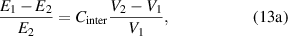
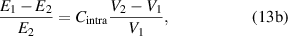
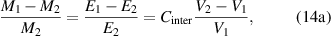
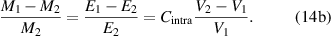
In the glassy state of an amorphous polymer, an isometric free volume is expected during the dynamic glass transition at Tg [57]. Therefore, a critical value of the free volume is expected to facilitate glass transition [57]. The FH solution theory was introduced to describe the free volume, in which the voids act as solvent molecules in glassy systems. Here, the thermodynamics of glassy matter, which comprises an amorphous polymer and a free volume, is governed by the FH solution theory to formulate the dynamic equilibrium of the free volume. Taking inspiration from the previous study on the phenomenological two-state, two-(time)scale model, which postulated the existence of two separate 'states' of low-temperature 'solid' and high-temperature 'liquid' [76], a thermodynamic equilibrium of dense-dilute two 'phases' has been developed. Based on the FH solution theory, when the free volume acts as a poor solvent, its size decreases, resulting in the phase separation of glassy matter during the cooling process whose temperature decreasing from above to below Tg . However, when the free volume acts as a good solvent, its size increases, resulting in microphase separation of the glassy matter during the heating process whose temperature increasing from below to above Tg .
We assume that glassy matter is a mixture of two interconvertible phases: a dilute phase of glassy matter and free volume, as well as a dense phase of glassy matter. The fractions of the dilute and dense phases are denoted by  (where
  =
= ) and
) and  (where
  = 1−
= 1− ), respectively, as shown in figure 9(a). According to the dynamic equilibrium of phase separation, the Gibbs free energy per molecule (G) of an athermal nonideal mixture is the sum of the contributions from both phases, as follows,
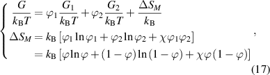
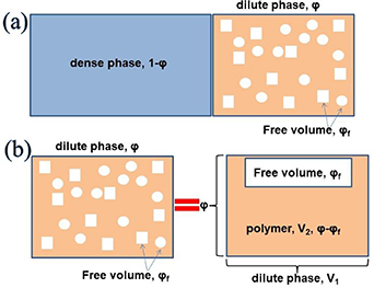
Figure 9. Schematic illustrations of glassy matter system, which is originated from the dilute and dense phases, based on the thermodynamics in solution theory. (a) Schematic illustrations of dynamic equilibrium of dilute and dense phases in glassy matter system. (b) Schematic illustrations of dynamic equilibrium of polymer and free volume in dilute phase.
Download figure:
Standard image High-resolution imagewhere  and
and  are the Gibbs free energies per molecule of dilute and dense phases, respectively,
  is the Boltzmann constant, ΔSM
is the mixing entropy, T is the temperature, and
is the Boltzmann constant, ΔSM
is the mixing entropy, T is the temperature, and  is the interaction parameter between two phases.
According to equation (17), the Gibbs free energy per molecule (G) of an athermal non-ideal mixture can be rewritten as follows,
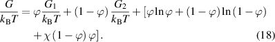
Based on equation (18), the chemical potential of the two phases can be obtained as,
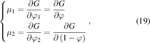
where  and
and  are the chemical potentials per molecule in the dilute and dense phases, respectively.
Owing to the dynamic equilibrium of the two phases, the chemical potential of the dilute phase is equal to that of the dense phase, that is  =
=  , leading to the following expressions,
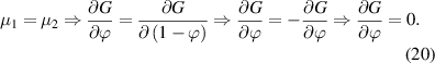
Substituting equation (20) into (18) yields the following expression,
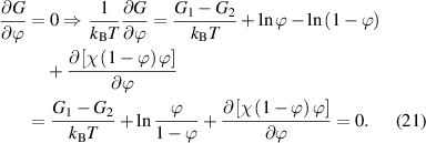
Owing to the function of 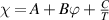 , the equation can finally be expressed as [38, 77]:
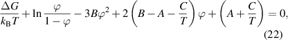
where  is the enthalpy change per molecule transformed from the dense phase to its dilute one. Meanwhile,
  is always used to present the enthalpy change based on the thermodynamics in solution theory. Therefore, the parameter of
  is derived from the enthalpy change of glassy matter, based on the dynamic equilibrium of dilute and dense phases.
In contrast, the specific volume ( ) of the dilute phase is incorporated from the mixture of a glassy matter and free volume, where the fractions are
  and
and  , respectively, as shown in figure 9(b).
The mixing of glassy matter and free volume in the dilute phase follows the rule of mass conservation,
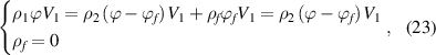
where  and
and  are the densities of the dilute phase (a mixture of glassy matter and free volume) and dense phase (pure glassy matter), respectively.
Therefore, equation (23) can be rewritten as follows,
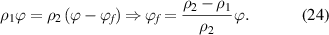
In the dilute phase, there is a dynamic equilibrium of mass conservation before and after mixing between the glassy matter and the free volume, of which the density is assumed to be zero in comparison with that of the glassy matter,  , thus,
where  denotes the free volume. The parameter
  can be determined using the fraction of the dilute phase (
 ).
).
Therefore, both the free volume ( ) and free-volume fraction (
 ) can be obtained based on equations (22), and (25), in which
  and
and  are derived from the enthalpy and entropy functions, respectively.
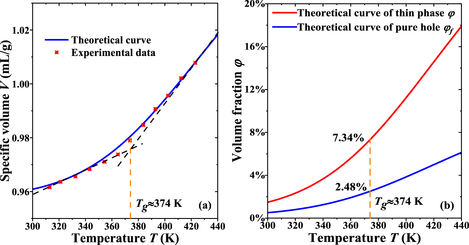
One set of experimental data [36] for an amorphous polymer was used to verify the analytical results generated using the proposed models, based on equations (22) and (25). Different parameters in the calculations based on equations (22) and (25) are listed in table 1. Based on the experimental results [36], the density ratio of the dilute phase to the dense phase can be obtained as follows,
Table 1. Values of parameters used in equations (22) and (25) for free-volume concentration.
| ΔG (kJ mol−1) | V1 (ml g−1) | V2 (ml g−1) | A | B | C (K) |
|---|---|---|---|---|---|
| 4.693 | 1.453 | 0.956 | −3.769 | −6.286 | 1883.7 |
Based on equation (24), the ratio  can be obtained as follows,
Figure 10(a) plots the analytical and experimental results [36] of specific volume as a function of temperature, where Tg
= 374 K. Furthermore, the constitutive relationships of dilute phase volume and free-volume concentrations ( and
and  ) as a function of temperature are plotted in figure 10(b). The results show that the dilute phase and free-volume concentrations (
 and
and  ) are 7.34% and 2.48%, respectively, at Tg
= 374 K.
) are 7.34% and 2.48%, respectively, at Tg
= 374 K.

Figure 10. Comparisons between analytical results using equation (27) and experimental data [36] of the specific volume as a function of temperature, where the glass transition temperature is 374 K. (a) Specific volume-temperature curve. (b) Analytical curves of dilute phase and free-volume concentrations ( and
and  ) as a function of temperature.
Download figure:
Standard image High-resolution imageRandom close packing is a mathematical concept used to characterise the maximum volume fraction of solid objects obtained when they are packed randomly. The random close packing of circles in two dimensions yields a theoretical packing density of 0.886441 [78]. Additionally, random close packing of spheres in three dimensions gives a packing density of 0.64–0.65 [78–80], with an expression of exact packing density reported in the past works [78]. Random close packing is an interesting and important physical and mathematical issue, especially for amorphous matter and its connection to glass transition.
Furthermore, the major difference between random close packing model and AG domain size model is summarised as follows. The free volume fraction of random close packing model applied to all types of glass transitions, including α-relaxation and β-relaxation, according to the previous reports [70, 81]. Conversely, it is found that there are two types of free volumes: grey regions for the free volume (Vvib) responsible for the vibrational motion of segments (β-relaxation) and also play an essential role for the delta transition (δ-transition) of monomer; and white regions (Vfree) for the free volume available to the segments undergoing glass transition (α-transition), as shown in figure 8. Additionally, the coordination number of the random close packing was 12 or 6, whereas that of the AG domain size model was 4. Therefore, random close packing model is used to characterise the free volumes of Vvib and Vfree, while the Vfree = 2.48% is the free volume available to the segments undergoing glass transition, which is applied to the α-transition.
4. Condensed constant and its connection to bivariate transition probability
Analogous to the Boltzmann constant ( = 1.3806 × 10⁻²³ J K−1, in thermodynamics, which relates the average relative kinetic energy of a particle with the temperature) and gas constant (R = NA
·
= 1.3806 × 10⁻²³ J K−1, in thermodynamics, which relates the average relative kinetic energy of a particle with the temperature) and gas constant (R = NA
· = 8.314 J mol−1·K, which is the proportionality constant used to relate the energy scale to the temperature scale, when one mole of particles is considered, where NA
= 6.02 × 10²³ is the Avogadro constant), it is expected that there is a condensed constant (C) to relate the activation energy scale (Ea
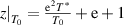
) to the temperature scale (T) for glassy matter at the condensed-matter scale and in temperature range from T0 to Tg
, that is, Ea
= C·T (T0 ⩽ T ⩽ Tg
). According to a previous study [35], the activation energy and volume functions play synergetic roles in determining the transition probability of glassy matter. Because the free volume concentration (
= 8.314 J mol−1·K, which is the proportionality constant used to relate the energy scale to the temperature scale, when one mole of particles is considered, where NA
= 6.02 × 10²³ is the Avogadro constant), it is expected that there is a condensed constant (C) to relate the activation energy scale (Ea
) to the temperature scale (T) for glassy matter at the condensed-matter scale and in temperature range from T0 to Tg
, that is, Ea
= C·T (T0 ⩽ T ⩽ Tg
). According to a previous study [35], the activation energy and volume functions play synergetic roles in determining the transition probability of glassy matter. Because the free volume concentration ( ) is a constant at Tg
, effect of the transition probability (
) is a constant at Tg
, effect of the transition probability ( ) of the volume function on glassy matter remains constant. According to hard-sphere free-volume theory [61], the average distribution of the volume function (
 ) in glassy matter is associated with the free-volume concentration (
 ), as follows,
where  is the total volume of glassy matter and
  is a numerical factor that corrects the superposition of free volumes [61].
The conditional probability of the volume function ( ) at Tg
(or
) at Tg
(or  ) is then obtained as follows [61],
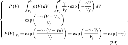
where  is the initial total volume occupied by all the molecules and remains constant as
  .
.
Therefore, the transition probability of the volume function is obtained as  = e−γ
. Furthermore, the transition probability of glassy matter is a bivariate transition probability function, (
= e−γ
. Furthermore, the transition probability of glassy matter is a bivariate transition probability function, ( ), which involves two variables: activation energy (
 ) and volume (
 ). Although the transition probability of the activation energy (
 ) is governed by a binomial (or Bernoulli) distribution, the sigmoid function is often used to describe the effect of the activation energy (
 ) on the transition probability. Therefore, the conditional probability of the activation energy (
 ) in glassy matter is described by the Eyring equation [45],
where  is the change in activation energy at Tg
.
is the change in activation energy at Tg
.
Combining equations (29) and (30), we obtain the bivariate transition probability ( ), in which the individual probability functions of the independent random variables can be expressed without reference to other variables at Tg
as follows:
), in which the individual probability functions of the independent random variables can be expressed without reference to other variables at Tg
as follows:
For most cases where  = 0 [45] and
  = 1 [61], equation (31) can be expressed as follows,
Consequently, equation (32) agrees with equation (12), where the transition probability is  .
.
For  > 0 and
  , equation (32) can be expressed as follows:
Here, a condensed constant (C) is introduced, where CT ( ) is used to represent the activation energy of glassy matter at the condensed-matter scale, that is,
 (
( ). Thus, equation (33) can be rewritten as,
where  and
and  = 1.73 [34].
Therefore, a condensed constant (C) is expressed as:
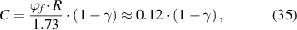
where  = 2.48% and
  = 8.314 J (mol·K)−1.
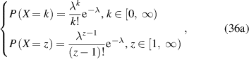
It should be noted that there is a constitutive relationship between the domain size (z(T) = k + 1) and temperature (T) as a function of the number of times an event occurs (k), that is, z(T) =  = k + 1, where
  and
and  originate from the AG domain size model [45]. Here, the
  = k + 1 could be not an integer, due to that the parameter of domain size (z(T)) can be not an integer.
The probability density function with respect to the domain size (z) or temperature (T) can then be expressed as follows,
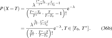
As  = e + 1, there is a constitutive relationship between the glass transition temperature (Tg
) and the AG domain size (z) as follows [45],
= e + 1, there is a constitutive relationship between the glass transition temperature (Tg
) and the AG domain size (z) as follows [45],
where are  = 1 and
  = ∞ [45].
The curve of Poisson distribution function with respect to the AG domain size (z) has the same shape as that of the function of temperature (T), as shown in figure 11.
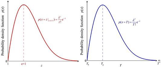
Figure 11. Analytical curve of probability density function of Poisson distribution as functions of domain size (z) and temperature (T), respectively.
Download figure:
Standard image High-resolution imageTherefore, there is the same scale range for the domain size (from  = 1 to
  ) and temperature (from T0 to T*), as follows [45],
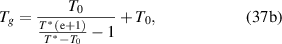
According to equation (38), it can be shown that  . Here, the domain size (z) has a finite range from 1 to
  , that is,
  , where both T0 and T* parameters can be experimentally measured. Based on equation (36), the probability density as a function of the AG domain size (z) can be expressed as follows,
Finally, its cumulative distribution function is obtained as,
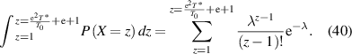
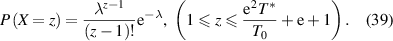
According to the experimental results of T0 and T* [82],  can be calculated, where the parameters used in the calculation are listed in table 2,
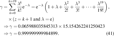
Table 2. Values of parameters used in the calculations of  for PS and PoCS.
| Types | T* (K) | T0 (K) |
|
kmax( ) ) | References |
|---|---|---|---|---|---|
| Polystyrene (PS) | 773 | 330 |
 ≈ 21 ≈ 21 | 20 | [82] |
| Poly o-chlorostyrene (PoCS) | 773 | 358 |
 ≈ 20 ≈ 20 | 19 | [82] |
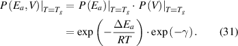
By combining equations (35) and (40), the numerical factor can be derived to correct the superposition of free volume (γ). This correction factor is characterised using the cumulative Poisson distribution of probability density function, and is found to be γ = 0.999999999984899 (where  = 20 and k =
  = 19), based on equation (41). Finally, a condensed constant (C) is calculated as C= 1.501 × 10⁻¹¹ J·mol−1·K−1, according to the equation (35) and γ = 0.999999999984899. As shown in figure 12, a condensed constant is a given constant indicating that the activation energy of condensed matter is determined solely by temperature, that is,
  (
( ), analogous to the Boltzmann (kB) and gas (R) constants for molecular dynamics and continuum mechanics, respectively.

Figure 12. Condensed constant (C) for the scale of condensed matter, analogous to that of the Boltzmann (kB) and gas (R) constants for scales of molecular dynamics and continuum mechanics, respectively.
Download figure:
Standard image High-resolution image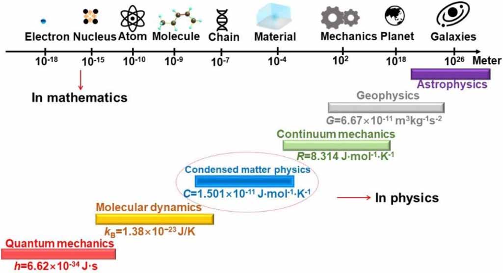
5. Conclusions
This study aimed to answer the question on the nature of glassy state. This is one of the greatest scientific conundrums in condensed-matter physics. The convergence of physics and chemistry in the dynamic glass transition of glassy matter has been achieved to unify the laws of physics at the condensed-matter and molecular scales, leading to dynamic fluctuations and scaling effects. Three key contributions can be summarised as follow. First, glassy matter is a dynamically condensed matter, of which the physics meets chemistry at the glass transition temperature. Glass transition is a dynamic fluctuation of glassy matter, giving rise to a scaling effect owing to the interplay of interdisciplinary complexity at the condensed and molecular scales. There are two dynamic equilibria for the glass transition, the dynamic equilibrium of the order-to-disorder free energy, and the dynamic cooperativity of the domain size for molecular entanglement. It was verified that nearly 72 monomers relax cooperatively and synchronously at Tg
. Second, the connection between the glass transition and free volume is derived from dynamic chaos and mathematical fractal. The scaling effect in the volume function results from dynamic fluctuation in chaos and dimensional difference in fractal. Physical insights for the free volume reveal that the free volume is governed by the Einstein mass-energy equilibrium. Fractal insight for the free volume reveals that it is governed by self-consistent iterations, resulting in a time-space correlation between the glass transition and the free volume. A phenomenological free-volume fraction of 2.48% was maintained constant at Tg
, according to the dynamic equilibria of enthalpy and entropy in the FH solution theory. Third, a condensed constant ( ) is obtained using the bivariate transition probability function of activation energy and volume functions, where the transition probability of the volume function is maintained at a constant value of e−γ
, and the transition probability of activation energy is also determined by the free-volume concentration according to the Einstein mass-energy equilibrium. Based on the bivariate transition probability (e−1) of activation energy and volume functions at Tg
, a condensed constant (
) is obtained using the bivariate transition probability function of activation energy and volume functions, where the transition probability of the volume function is maintained at a constant value of e−γ
, and the transition probability of activation energy is also determined by the free-volume concentration according to the Einstein mass-energy equilibrium. Based on the bivariate transition probability (e−1) of activation energy and volume functions at Tg
, a condensed constant ( ) is obtained as C= 0.12(1−γ) = 1.501 ×10⁻¹¹ J·mol−1·K−1, analogous to that of the Boltzmann (kB) and gas (R) constants. It is expected that the activation energy (Ea
) of glassy matter is solely proportional to the temperature (T) at the condensed-matter scale, that is,
) is obtained as C= 0.12(1−γ) = 1.501 ×10⁻¹¹ J·mol−1·K−1, analogous to that of the Boltzmann (kB) and gas (R) constants. It is expected that the activation energy (Ea
) of glassy matter is solely proportional to the temperature (T) at the condensed-matter scale, that is,  (
( ), where
  is a condensed constant. Furthermore, based on the scaling law, this study tries to provide an insight into the overarching question 'Can the laws of physics be unified?', which was resolved through the reconciliation of physics and chemistry. The scaling effect is governed by the interplay of interdisciplinary complexities at the condensed-matter and molecular scales, which are determined by the thermodynamics of inter-molecular (phase separation) and intra-molecular (microphase separation) cohesions, respectively. These effects manifest from the dynamic fluctuation of the glassy transition.
Acknowledgments
This work was financially supported by the National Natural Science Foundation of China (NSFC) under Grant Nos. 11725208 and 12332010.
Data availability statement
No new data were created or analyzed in this study.