

Abstract
This review examines the biological physics of intracellular transport probed by the coherent optics of dynamic light scattering from optically thick living tissues. Cells and their constituents are in constant motion, composed of a broad range of speeds spanning many orders of magnitude that reflect the wide array of functions and mechanisms that maintain cellular health. From the organelle scale of tens of nanometers and upward in size, the motion inside living tissue is actively driven rather than thermal, propelled by the hydrolysis of bioenergetic molecules and the forces of molecular motors. Active transport can mimic the random walks of thermal Brownian motion, but mean-squared displacements are far from thermal equilibrium and can display anomalous diffusion through Lévy or fractional Brownian walks. Despite the average isotropic three-dimensional environment of cells and tissues, active cellular or intracellular transport of single light-scattering objects is often pseudo-one-dimensional, for instance as organelle displacement persists along cytoskeletal tracks or as membranes displace along the normal to cell surfaces, albeit isotropically oriented in three dimensions. Coherent light scattering is a natural tool to characterize such tissue dynamics because persistent directed transport induces Doppler shifts in the scattered light. The many frequency-shifted partial waves from the complex and dynamic media interfere to produce dynamic speckle that reveals tissue-scale processes through speckle contrast imaging and fluctuation spectroscopy. Low-coherence interferometry, dynamic optical coherence tomography, diffusing-wave spectroscopy, diffuse-correlation spectroscopy, differential dynamic microscopy and digital holography offer coherent detection methods that shed light on intracellular processes. In health-care applications, altered states of cellular health and disease display altered cellular motions that imprint on the statistical fluctuations of the scattered light. For instance, the efficacy of medical therapeutics can be monitored by measuring the changes they induce in the Doppler spectra of living ex vivo cancer biopsies.
Export citation and abstract BibTeX RIS

Original content from this work may be used under the terms of the Creative Commons Attribution 3.0 license. Any further distribution of this work must maintain attribution to the author(s) and the title of the work, journal citation and DOI.
Recommended by Dr Masud Mansuripur
1. Introduction: life and disease at low Reynolds number
1.1. Life at low Reynold's number
At a symposium held in honor of theoretical particle physicist Victor Weisskopf in 1976, the Nobel laureate Edward Purcell delivered a talk titled Life at Low Reynold's Number, publishing a paper the following year with the same title [1]. The purpose of the talk was to illustrate and explain how the physical environment experienced by micron-scale living things is radically different than the world we experience. The deciding factor is Reynold's number, the ratio of inertial forces relative to viscous forces
where ρ is the density, v is the velocity, a is the size (assuming a sphere), η is the dynamic viscosity and ν is the kinematic viscosity. The values of viscosity for water are η = 1 × 10⁻³ Pa·s and ν = 1 × 10⁻⁶ m2 s−1. For instance, the Reynold's number for a 1 μm bacterium swimming at 1 μm s−1 is Re = 1 × 10⁻⁴, while for a 10 mm tadpole swimming at 10 mm s−1 it is Re = 100. The tadpole lives in the world of Newton's law (F = ma) and swims by accelerating water. In contrast, the bacterium lives in a world without inertia and swims by asymmetric shear movement that is more like crawling through water. The negligible role of inertial forces for micron-scale living things, or micron-scale objects inside living things, means that everything moves instantaneously at their terminal velocity—Newton's second law is inoperable on practical time scales. Velocities respond instantaneously to changes in forces balanced by drag.
The consequence of low Reynold's number for life in this micro-world is the dominance of diffusion as the primary mechanism of transport rather than drift. However, inside the cytosol of a cell a form of active drift becomes dominant over diffusion through molecular action-reaction forces operating by, and on, cellular infrastructure like the cytoskeleton. Intracellular drift is an active process, far from thermal equilibrium, driven by energetic processes fueled by energetic molecules of ATP and GTP. Molecular motors [2, 3], hydrolyzing ATP, walk on components of the cytoskeleton and drag along organelle and vesicle cargo. Similarly, the persistent growth and collapse of supporting cytoskeletal structures are enabled by hydrolyzing GTP. The enthalpy of ATP hydrolysis at physiological temperature is 0.37 eV, and the energy density per ATP molecule has an equivalent temperature of  . In comparison, the effective temperature Teff for active organelle walks can be assessed from an effective diffusion coefficient as
where v0 is speed (on the order of microns per second) and τ is the persistence time (on the order of seconds). If the speed of an organelle with a 0.1 μm radius is 1 μm s−1 for a persistence length of 1 μm at an intracellular viscosity of 0.1 Pa·s [4], then the effective temperature is about 12 000 K. In terms of energy dissipation, if the force on the organelle is 6 pN (typical of the force applied by a molecular motor on an organelle), then the average power dissipated is approximately 37 eV s−1 which is the hydrolysis of approximately 100 ATP molecules per persistence length [5, 6]. These rough approximations point to highly non-equilibrium conditions for intracellular transport, although effective thermal properties for systems far from equilibrium must be interpreted with caution. Molecular motors are not thermal engines but rather are chemical engines, which is why effective temperatures can be so large.
Intracellular transport, driven either by molecular motors or by cytoskeletal restructuring, exhibits high persistence for both speed and direction. Persistent transport, also known as processive transport (see section 3), has finite persistence times during which velocity can be steady and correlated during periods between stochastic changes. Processive intracellular transport consists of runs and pauses, not unlike the run and tumble motion of bacteria. Processivity defines the number of steps taken before a motor detaches, or it expresses the prevalence of directed versus random steps. The run and pause motion of intracellular transport creates a continuous-time flight that has many properties of a random walk, but with piecewise continuous runs rather than jumps (see section 2). Light scattered from intracellular constituents executing persistent walks acquires small Doppler shifts that range from milli-Hertz to tens of Hertz. The transport inside cells and tissues is essentially isotropic, and the superposition of many different transport processes across many scales ensures that the average Doppler shift vanishes. However, the interference and beats among all the Doppler frequencies produce statistical fluctuations in the scattered light intensity that carries information about the subcellular dynamics that can be extracted through fluctuation spectroscopy (FS) (see section 2).
1.2. Dynamical disease
From a dynamical system point of view, cellular health is a time-dependent dynamic equilibrium that balances fluxes among a hierarchy of cellular components and subcomponents. The healthy state is a generalized limit cycle within a dynamical phase space of high dimensionality composed of all the dynamical coordinates (variables) of the complex system. The idea of 'normal' health is not a single point in this state space (or health space), rather it is a cloud of points that inhabit a sub volume restricted within nominal ranges in the state-space description. In this context, disease is a deviation of this state-space cloud from its usual range to new regions within the space. Homeostasis, or feedback, confines the limit cycle to its healthy region. However, when variables change, either through genetic mutation, or through viral or bacterial attack, or through environmental stress and changing microenvironments, or though shocks to the system, then the dynamic equilibria can shift out of the nominal healthy range. Because of the high dimensionality of this health space, the volume of 'unhealthy' conditions far exceeds the volume of healthy conditions, causing a wide variety of possible unhealthy behaviors.
The study of dynamical disease, viewed as nonlinear dynamical systems, was initiated by Art Winfree and independently by Leon Glass and Michael Mackey, among others. Nonlinear dynamics can describe circadian rhythms [7], biological feedback control systems [8], heart arrythmias [9, 10], neurodegenerative diseases [11–13], and hematological disease [14, 15]. These dynamical diseases are macroscopic at the tissue or organ scale and are studied in low dimensions with typically less than a dozen dynamic variables [16]. In contrast, cancer is a dynamical disease at the cellular and subcellular level with a high-dimensional state space composed of dynamical variables associated with genetic networks [17–20] that can have high dimensionality. Dynamical processes also occur within the cell, involving signaling pathways and the cell cycle [21–23].
At the microscopic level there is an astonishing array of dynamical systems associated with cellular function and health. A major class of these dynamical systems involve motor proteins that execute directed motion along structure elements. These include kinesin and dynein molecular motors [24] that move along microtubules [25] at speeds of microns per second, myosin molecular motors [26, 27] that move along actin [28, 29], DNA helicase [30–32] and RNA polymerase [33] that travel along DNA, ribosomes [34, 35] that move along m-RNA, and MMP-1 proteins [36] that travel along extracellular collagen. In addition, the formation of the structural elements themselves (such as microtubules, actin filaments and intermediate filaments) involve the dynamically fluctuating formation and collapse of long-range assemblies through cytoskeletal restructuring [37] and adhesions [38–40] that exert forces on subcomponents of the cell and on the cell membrane causing directed movement (drift) superposed on fluctuations. Dramatic examples of concerted and collective motions caused by cellular dynamics are the formation of the mitotic spindle [41], the separation of the chromosomes, and cytokinesis [42] during mitosis [43–45] as cells divide at speeds of tens of nanometers per second. Another example is endocytosis [46, 47], as dynamic reassembly of the actin cortex generates endocytic vesicles from the cell membrane that move rapidly with speeds as high as tens of microns per second. Among the longest-range consequences of cellular dynamics are cell crawling, immune cell infiltration, and metastasis [48, 49] that occur over scales of tens of microns and longer.
Many disease states involve the cellular cytoskeleton and its associated molecular motors. For instance, molecular motors can participate in cancer processes, such as a possible connection between KIF11 and prostate cancer [50], and between KIF11 and Taxol resistance [51]. Molecular motors also can participate in neurogenerative disease, such as a functional interaction between kinesin-I and amyloid precursor protein in Alzheimer's disease [52], in phosphorylation in Huntington's disease [53], and in axonal transport in Alzheimer's disease [54, 55]. Metabolism is central to all cellular processes, and modifications in motors can affect dynamin and glucose uptake [56] and mitochondrial fusion and fission [57]. Tissue dysfunction likewise is affected, as in myosin-5B and microvillus inclusion disease [58], and myosin motor dysfunction related to cardiomyopathy [59]. These modifications produce changes in cellular dynamics, either displaying modified cellular phenotypes that could help in the diagnosis of disease, or providing dynamic biomarkers that signal how effectively treatments may be applied.
The cytoskeleton provides a template for many cellular processes, and alteration of normal cytoskeleton function can have deleterious effects. For instance, there are connections between microtubules and neurodegenerative disease such as Krabbe's disease [60], Huntington's disease [61, 62] and multiple sclerosis and Alzheimer's disease [63]. Alzheimer's disease has also been associated with synaptic actin [64]. Connections have been assessed between integrin and renal disease [65]. Intermediate filaments and desmosomes affect monogenic diseases (severe skin fragility, myopathics, neurodegeneration, and premature ageing) and polygenic diseases (liver and inflammatory bowel disease) characterized as 'mechanical weakness' disorders [66]. Keratin is related to liver disease [67]. Intermediate filament aggregates relate to Charcot–Marie–Tooth disease and amyotrophic lateral sclerosis, while tau inclusions and frontotemporal dementia relate to parkinsonism, progressive supranuclear palsy and corticobasal degeneration [68]. Muscle activity is affected by actin in congenital myopathy [69, 70] and cardiomyopathy [71]. These connections between disease state and the structure and dynamics of cells provide an opportunity to use dynamic probes such as dynamic light scattering (DLS) to assess health and disease.
Just as disease is characterized by a change in intracellular motion, the treatment of disease also modifies motions. Antimitotic drugs inhibit the functions of the cytoskeleton which affects the dynamic restructuring of the cytoskeleton as well as cellular mechanical properties. For instance, the cytochalasins degrade the actin cortex which decreases the stiffness of the cell membrane and causes increased membrane fluctuations [72]. Taxol stabilizes tubulin polymerization, preventing microtubule treadmilling [73]. Colchicine degrades microtubules, decreasing the persistence of molecular motors and organelle transport [74]. Motor poisons affect the functioning of motors associated with the kinetochore during mitosis [75]. Cellular adhesions are critical elements in the maintenance of mechanical homeostasis and are targets of applied therapies [76]. In contrast to the direct mechanical effects of cytoskeletal and molecular motor drugs, the desired endpoint of many cytotoxic chemotherapies is induced apoptosis. Apoptosis is a highly energetic process in which the cell systematically disassembles itself and is associated with enhanced vesicle transport [77] and the fragmentation of the cell into apoptotic bodies [78]. These processes are characterized by dramatic short-range and long-range motions. Targeted therapies, such as tyrosine kinase inhibitors, are directed to specific proteins in intracellular signaling pathways, including mutations in KRAS, BRAF, mTOR, PI3K, all of which have downstream cascades that affect cellular motions such as FAK (cytoskeletal reorganization), PRK-1 (membrane trafficking), Citron and Septins (cytokinesis), P140 (membrane ruffling), Cofilin (actin nucleation), NHE1 (focal adhesions), MLC (actomyosin contraction), CEP2/3 (regulation of the cytoskeleton), aPKCs (MTOC orientation), OP18 (microtubule growth), IQGAP (cell–cell adhesions), among many others. In all of these examples, modified function induces modified motions of and within the cells. Consequently, these changes in motion can be detected using light scattering techniques to monitor the state of health of living tissues and the efficacy of treatment of disease.
1.3. Dynamic 3D tissue beyond 2D cell culture
Natural disease occurs in a natural three-dimensional environment. However, two-dimensional cell culture has been the mainstay of cellular biology for over half a century. Fundamental biological research, as well as applied research for drug development, have been pursued in the context of cells modified to grow on flat hard surfaces with altered shapes and sizes and with minimal contact to other cells [79–82]. Over the past few decades, growing evidence shows that these artificial environments modify the structure and function of cells with important consequences for the study of biologically relevant processes. There are different genetic expression profiles [83–85], different intercellular signaling [86–89], and different forces attaching them to their environment [90–92]. Furthermore, the tumor microenvironment exerts a dominant influence on the effectiveness of chemotherapy [80, 93, 94], including the presence of immune cells that infiltrate the tumor in vivo and are indicative of patient prognosis [95].
The three-dimensional microenvironment is particularly important for understanding (and recapitulating) tumor behavior [93, 94, 96], especially regarding the emergence of drug resistance [97–99]. For example, it has been shown that indiscriminate cytotoxic drugs damage the tumor microenvironment and can actually promote tumor growth [100]. Therefore, maintaining the three-dimensional structure of tumor biopsies is imperative when studying tumor physiology. Ideally, testing the sensitivity of a patient to prescribed cancer therapeutics would use techniques based on living ex vivo biopsies that retain the full 3D microenvironment, including signatures of intracellular transport. For these reasons, studies of dynamic processes in tumors should rely on three-dimensional primary tissue rather than on cell culture.
To probe three-dimensional tissue, optical approaches have several advantages. Light scattering is a remote sensing technique that is nondestructive. In translucent tissue that is not highly absorptive, infrared light can penetrate up to 1 mm ballistically, and can penetrate up to many centimeters diffusively. While direct imaging is limited to depths less than several hundred microns [101–103], several deep-tissue probes exist that can extract dynamic information, such as diffuse correlation spectroscopy [104], digital holography [105], optical coherence tomography (OCT) [106] and diffusing wave spectroscopy (DWS) [107]. There have also been recent advances using superresolution microscopy to evaluate intracellular dynamics at shallow depths [108] with efforts to extend superresolution to deep tissue [109–111]. These optical techniques enable dynamic processes to be investigated deep inside tissue, far from perturbing surfaces, in a biologically relevant context.
2. Light transport: coherent light scattering
The coherent properties of light is a sophisticated topic of study in physics [112] and provides a powerful tool for experimental science and sensing [113]. When light with at least partial coherence scatters from moving objects it acquires information pertaining their size, shape and motion relative to the directions of the incident and scattered light rays or photons. When there are many objects with complex structures and motion, the coherent superposition of the scattered light is conveniently studied through statistical optics [114] where one of the salient characteristics of ensemble light scattering is the observation of coherent speckle [115, 116] that may have both static and dynamic components [117]. The study of dynamic speckle is performed through FS [118] which yields information on the properties of the light-scattering objects. Therefore, coherent light scattering is particularly helpful for the understanding of cellular and intracellular motion in living tissue.
2.1. The Doppler effect in light scattering
Light scattered from moving scatterers acquires a small frequency shift that depends on the relative direction of motion of the scatterer and the momentum change of the light. This effect [119] was proposed in 1842 by Christian Doppler [120] and independently in 1848 by Armand Fizeau [121]. The relativistic form for angular scattering was first derived in 1905 by Einstein [122]. For an incident photon with k-vector  that scatters into
  from a particle moving with velocity
  , the Doppler shift upon scattering can be described as
where the Lorentz factor is  , and where the 'momentum transfer' is

and
The scattering geometry is shown in figure 1. The scattered k-vector  is characterized by the angle θ relative to the direction of
  , and the momentum transfer
  is described by the angle ϕ and
  . The shifted angular frequency of the scattered photon is
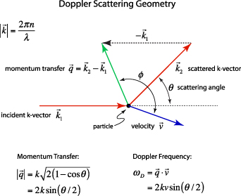
Figure 1. The incident k-vector in Doppler light scattering is deflected through an angle θ. The difference between the incident and scattered k-vector defines the momentum transfer, called the q-vector. The angle between the q-vector and the particle velocity is ϕ, and the Doppler frequency shift is given by the inner product of the q-vector with the particle velocity.
Download figure:
Standard image High-resolution imageand the low-velocity expansion of the Doppler frequency is
showing the direct relationship to the scattering vector and the particle velocity. The Doppler frequency shift is then
An equivalent description of the Doppler light scattering process uses the phase of the scattered wave, for which the scattered field can be expressed as [117]
where the time-dependent displacement is Δxt
= x(t) − x(0). In the final expression for a given momentum transfer  , there is only one degree of freedom, designated as the variable x, which is the projection of the displacement of the particle onto the direction of the vector
  . Therefore, low-frequency Doppler frequency shifts are detected through phase-sensitive interferometric detection of one-dimensional particle displacements. Displacement and velocity are related simply through time, and time-dependent fringe intensity modulation is equivalent to a Doppler beat frequency.
2.2. Ensemble Doppler spectroscopy
The angle θ in equation (2.6) is set by the optical scattering geometry, but the angle ϕ is related to the motion of the scattering objects. In the case of intracellular motions, these angles are isotropically oriented, and the average Doppler frequency shift is zero. However, the distribution of object speeds and orientations are contained in the fluctuations in the Doppler frequency spectrum. Therefore, ensemble FS [118, 123, 124] becomes the primary means to extract information about the velocity distributions within the scattering volume. FS operates in the statistical optics limit of a large number of scattering objects producing a large number of interfering partial waves.
2.2.1. Partial wave sums.
When coherent light illuminates a group of N discrete scattering objects, the total scattered field is
The amplitudes Ei
of the fields are real-valued, and the phases ϕi
span the unit circle modulo 2π. In statistical optics, the amplitudes and phases are stochastic variables. For a Gaussian probability distribution with variance  , when the phase is uniformly distributed on 2π, the random sum describes Gaussian diffusion on the complex phasor plane.
The intensity from N sources without a reference field (homodyne detection) is
In the large-N limit, the second term averages to zero because of the random phases in the exponent [113], giving
where Is is the average squared field per scatterer. The average intensity depends linearly on the number N of sources as an incoherent sum. The fluctuations are

where the expression for  is
is
Because the field takes positive and negative values, the cross-terms average to zero, and the factor of two is the result of adding two random Gaussian distributions of equal variance. The variance of the fluctuating intensity is
and the fluctuations in the homodyne intensity are equal to the average intensity 
For a heterodyne condition
where ϕ0 is the reference phase [113], the intensity is
with an ensemble average

When the reference magnitude  is much larger than
  (i.e. a strong reference wave) then the heterodyne intensity fluctuations are

and the intensity fluctuations scale as the square root of the number of scattering sources.
2.2.2. Autocorrelation.
For homodyne detection without a reference field the intensity autocorrelation is the product of the intensity with itself [117]
neglecting terms of random phase in the large N limit. The ensemble average is
where the discrete sum is replaced by an integral over a joint probability distribution W(x,y,τ), and the variables x and y are the one-dimensional displacements relative to the direction of  . If the displacements of the particles are uncorrelated, then the joint probability distribution W(x,y,t) is separable and the sum is converted to the product of integrals
expressed as a spatial Fourier transform indexed by spatial frequency q that operates on the W function (the operation denoted by the small circle). This expression is the central statement of FS: the autocorrelation function of the fluctuations are directly related to the Fourier transform of the probability function W(x,t) that defines the time-dependent displacements of the particles.
For heterodyne detection with a reference field, the scattered field mixes with the reference to produce the net field
The time autocorrelation function averages the product of the field over a time-shifted field. In the limit of large N this yields [113]
The autocorrelation is an ensemble average of this quantity, where ensemble averages and time averages are equivalent under stationary statistics. The stochastic sum is evaluated using an integral
where Is is the average scattered intensity, FTq is a Fourier transform over spatial frequency, and W(x,t) is again the probability distribution of particle displacements. Therefore, W(x,t) is the central object of interest in the study of anomalous transport (see section 4). The homodyne autocorrelation is related to the heterodyne autocorrelation through the Siegert relation [125, 126]

where β is a factor related to the coherence contrast at the observation plane.
2.2.3. Wiener–Khinchine theorem.
A statistically stationary time-series f(t) is shown in figure 2(a) sampled by an exposure (integration) time texp at a periodic frame rate trep. A time-series analysis of the discretely sampled intensity can generate an autocorrelation function or a spectral power density. The Wiener–Khinchine theorem [127, 128] connects autocorrelation functions with spectral power density through

Figure 2. Dynamic light scattering autocorrelation and spectral density. (a) An intensity time series is sampled by a frame rate fps = 1/trep and an exposure time texp. The intensity is integrated over the exposure time. (b) The autocorrelation function varies between the average squared field and the squared average field. The slope at short delay is the inverse correlation time. A distribution of phase fluctuations produces an exponentially decaying autocorrelation. (c) The Fourier transform of the autocorrelation function produces the spectral density. A knee frequency is associated with the autocorrelation time. The floor of the spectral density at the Nyquist frequency is the integrated power between the Nyquist frequency and the detection bandwidth (inverse exposure time). Nyquist floors can be considerably higher than noise floor in active biological systems.
Download figure:
Standard image High-resolution imagewhere the heterodyne fluctuation power density is proportional to the spatial-temporal Fourier transform of the distribution probability functional W(x,t). Therefore, the autocorrelation function contains the same information as the spectral power density and the two may be viewed as equivalent descriptions. Autocorrelation functions are well-suited to characterize dissipative systems, but power spectra provide a different perspective. For instance, when a system has persistent drift, the associated Doppler frequency is represented directly in the spectrum. Therefore, FS is a useful tool for studying biological systems, consisting of different types of directed motion. In DLS, a classic transform pair is the exponential decay paired with a Lorentzian line shape
where AN is the noise floor of the autocorrelation. Classic diffusion of scatterers produces the decaying exponential autocorrelation function for light scattering. The Lorentzian line shape on a log–log graph has a low-frequency plateau, a characteristic knee frequency set by the decay rate of the autocorrelation function, and an inverse square roll-off to a Nyquist floor as shown in figure 2. Another important transform pair is the stretched decaying exponential and Lévy stable distributions (see section 4).
2.2.4. Non-stationarity and non-ergodicity in DLS.
Light scattering from living tissues is subject to non-ideal conditions that arise from its heterogeneous properties in both space and time [129–133]. Although the highly useful Wiener–Khinchine theorem holds for stochastic systems that have stationary statistics, living biological systems are prone to drifts in their properties over time, raising questions of when it is valid to apply the Wiener–Khinchine theorem to experimental time series and when it is not. Stationarity is defined as a stochastic system having probability distribution functions (PDFs) that are time-shift invariant. A slightly weaker constraint is called wide-sense-stationary for which the mean and the autocorrelation are time invariant, for which the Wiener–Khinchine theorem continues to hold. If the mean or autocorrelation of intensity fluctuations in a DLS measurement drift slowly relative to a sampling rate, then the drift can be compensated to convert the non-stationary time series to a stationary time series, and the Wiener–Khinchine theorem can be applied. However, if the drift rate is comparable to a sampling rate, then the Wiener–Khinchine theorem breaks down, and the spectral power density and autocorrelations functions are no longer related through a simple Fourier transform. In this case, Fourier transformation of the fluctuating intensities can still be performed, and the modulus-squared spectral functions averaged, but the resulting spectral function will have a 1/f noise characteristic at low frequency with high variability. Adjusting sampling rates in a DLS experiment on living tissues to bring the measurement system into the Wiener–Khinchine regime is a key design feature for such experiments. Living tissues experience slow drifts over minutes to hours corresponding to changes in nutrients or oxygen and possible changes in temperature. Therefore, sampling rates in the range of many per second for observation times extending from 10 to a 100 s are appropriate for maintaining the validity of the Wiener–Khinchine theorem for DLS experiments on tissues.
Ergodicity is another an important feature of a stochastic system when defining its light scattering properties [134]. Systems are called ergodic if they sample all their available configurations in sufficiently long times. For an ergodic system, the time averages of its properties are equal to ensemble averages. This important property allows time averages to stand in for spatial averages when analyzing experiments. Ergodic systems are stationary, but systems can be stationary without being ergodic. Such stationary but non-ergodic systems are the most common situation in light-scattering experiments on living tissue. The non-ergodicity of tissue dynamics arises for multiple reasons chiefly related to the spatial heterogeneity of tissue from the molecular scale through organelle and cytoplasm scale to the cellular scale and beyond. In this case, ensemble averages will not match isolated time averages. Non-ergodicity also arises from the wide range of intracellular and cellular speeds associated with the constituents of cells and tissues. Mitochondria, for instance, have a velocity PDF that has a root-mean-squared value of many microns per second, but the probability function is peaked at zero velocity for stationary mitochondria which are the most probable. A DLS experiment with a sampling time and an observation duration may not capture the slow changes of the slow mitochondria, and the stationary mitochondria generate a constant background scattering intensity so that autocorrelation functions asymptotically approach non-zero long-time values rather than zero means.
The non-ergodic properties of light scattering from tissue can be addressed experimentally by measuring broad-area speckle patterns, allowing both time averages and spatial averages to be performed. This approach has been used by Pusey et al [135, 136] to solve for the intermediate scattering function of a medium. For an ergodic system, the simple Siegert relation holds

where g(2)(q,t) is the normalized intensity autocorrelation function for spatial Fourier component q and lag time τ, β is a non-fundamental function of the optical apertures of the apparatus (for a single spatial mode β = 1), and f(q,τ) is the intermediate scattering function of the electric field autocorrelation function. However, this relationship is modified by a non-ergodic target where the intermediate scattering function is [135]
where the subscripts T and E are for time-average and ensemble-average, respectively. This allows a local f(q,t) to be derived by comparing the local time averages  to the ensemble averages over the speckle field
  (acting as a normalization factor) and to the non-constant component of the time-averaged second-order correlation. On the other hand, averaging equation (2.28) over the full speckle field can retrieve the simpler relationship equation (2.27) at the loss of local spatial variations.
2.3. Spatial coherence and speckle
The random movements of objects scattering light inside living tissue produce not only random phases in time but also in space. Therefore, DLS and FS are fundamentally associated with the phenomenon of coherent speckle. Examples of Gaussian speckle are shown in figure 3 for changing illumination radius w0 = 64, 32, 16 and 8 μm for z = 1 cm and λ = 500 nm with a field-of-view of 5 mm.
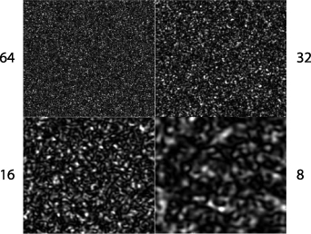
Figure 3. Speckle intensities for a random phase screen and changing illumination radius w0 = 64, 32, 16 and 8 μm for f = 1 cm and λ = 500 nm with a field-of-view of 5 mm.
Download figure:
Standard image High-resolution imageThe intensity distribution of fully-developed speckle is
with the important property  where the standard deviation of the intensity is equal to the mean intensity. The contrast of a speckle field is defined as
  and hence fully developed speckle has unity contrast.
The spatial correlations in intensity at an observation plane define the 'size' of speckles. For intensity at the emission plane given by I(x',y') the first-order normalized amplitude correlation coefficient (in the paraxial approximation) is
where the numerator is a Fourier transform on the paraxial phase factor. The second-order (intensity) normalized correlation function is defined as
which is related to the first-order correlation through the Siegert relation [126]
under the condition of full temporal coherence and Gaussian fluctuations. A common example is a Gaussian beam with intensity which has a lateral coherence diameter  for a beam width w0 and a wavelength λ observed at a distance z from the emission plane [113].
An alternate approach to defining spatial coherence is through the coherence area at the observation plane
where A is the source emitting area, and Ωs is the solid angle subtended by the source emitting area as seen from the observation point, if the angular spread of the light scattered from the illumination area is very broad. Larger distances and smaller pinholes produce larger coherence areas in a coherent optical system. For a Gaussian intensity distribution at the emission plane, the coherence area is
for a beam waist w0 at the emission plane.
A phase modulation must be associated with any intensity modulation through the Kramers–Kronig relations [137], with an example of a speckle hologram and its associated phase shown in figure 4. The hologram fringes are not parallel because of the varying phase of the speckle field, but the average spatial frequency is unaffected. When the hologram is numerically reconstructed, the side-band spatial frequency has a line shape determined by the speckle pattern. If the hologram is in the Fourier domain, a Fourier transformed sideband is in the image domain and reconstructs the image-domain speckle.
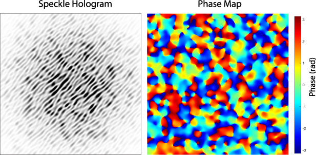
Figure 4. Speckle hologram and speckle phase. (a) A coherent plane-wave reference added to fully-developed speckle with unity contrast produces a speckle hologram. (b) The phase of the speckle varying through 2π.
Download figure:
Standard image High-resolution imageIn the speckle intensity field, there are locations where the intensity vanishes and the phase becomes undefined. In the neighborhood of such singular points, the phase wraps around it with a 2π phase range, creating an optical vortex [138]. Vortices come in pairs with opposite helicity (defined by the direction of the wrapping phase) with a line of neutral phase between them as shown in figure 5. In dynamic speckle, vortices are dynamic and move with speeds related to the underlying dynamics of the scattering medium [139]. Studies of singular optics [140] and structured illumination [141] create an active field of topological optics with applications in biological microscopy as well as material science.
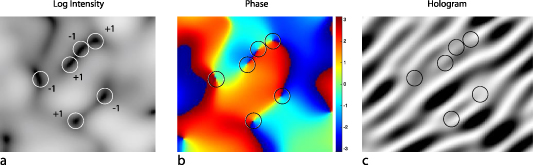
Figure 5. Optical vortex patterns. (a) Log intensity showing zeros in the intensity field where the circles highlight the intensity nulls which are the optical vortices. (b) Associated phase with a 2π phase wrapping around each singularity. (c) Associated hologram showing dislocations.
Download figure:
Standard image High-resolution image2.4. Light scattering from cells and tissues
Tissue is optically thick and has a physical scale that is much larger than the photon scattering length. Therefore, light that penetrates to a significant depth inside tissue experiences multiple scattering. At extreme depths, the light behaves diffusively, spreading as a diffusive front. However, at intermediate depths one can define average propagating intensities within the tissue through the effect of scattering on energy and momentum flux. The origin of light scattering is the optically heterogeneous refractive index discontinuities and gradients of the cellular, subcellular and extracellular components of tissue. The local structure of tissue also contributes as is seen so dramatically in the difference between the highly-scattering sclera (the white of the eye) and the transparent cornea that share the same composition of collagen, differing only in the arrangement of their collagen fibrils [142].
2.4.1. Optical properties of cells and tissues.
Cells and tissues comprise a heterogeneous mixture of constituents having a wide range of scales ranging from molecules (at the scale of nanometers) to layers of cells (at the scale of millimeters). The components have differing refractive indices that present a spatial optical refractive landscape that scatters light [143]. The smallest objects like organelles and vesicles cause Rayleigh scattering, while the largest objects, like cell layers, refract light as heterogeneous dielectric regions. In the intermediate regime, at the scale of the nucleus and other large organelles, or even the scale of single cells, the scattering is in the Mie scattering regime with higher probability of forward scattering but also with enhanced backscattering. One of the strongest sources of backscatter from tissue is from the cell scale associated with the cell membrane [144]. Even though the cell membrane volume is very small, it provides a relatively sharp interface between the internal cytosol and the external matrix.
A large literature exists that has explored the refractive indices of cellular constituents [145–151], which is partially summarized in table 1. Refractive index values within tissue range from water with n = 1.33 to dense lipids and dense RNA with n = 1.55. However, there is a high variability in refractive index values among cell and tissue types as well as differences among species, hence detailed studies of refractive index profiles in cells using quantitative phase microscopy need to be viewed within their own contexts [152–156]. To set an intuitive scale on backscattering from a planar refractive index contrast, the Fresnel reflectance coefficient for an index step of Δn = 0.08 on a background of n = 1.37 is 0.1%.
Table 1. Refractive index of cellular and tissue components at visible wavelengths.
| Cell component | Index of refraction | References |
|---|---|---|
| Cytoplasm | 1.37 | [157] |
| Lysosomes | 1.6 | [158] |
| Mitochondrion | 1.42 | [159] |
| RNA (nucleolus) | 1.55 | [160] |
| Nucleus | 1.39 | [157] |
| Cell membrane | 1.54 | [144] |
| Collagen | 1.43 | [161] |
| Cornea | 1.41 | [162] |
| Extracellular fluid | 1.35 | [163] |
| Tissue | 1.39 | [164] |
2.4.2. Light transport in tissue.
In single-scattering of light, the likelihood of scattering into an angle θ is given by the probability function p(θ) known as the phase function. The phase function is normalized  for scattering into 4π solid angle. A central property of light transport in tissue is the anisotropy factor, which is the average of the cosine of the scattering angle
To obtain intensity distributions in the intermediate regime of multiple small-angle scattering, the small-angle approximation (SAA) is appropriate for high anisotropy factor g in which most scattering is small-angle forward scattering, which is the case for most translucent biological tissues. The flux in this case is described as
where τ is the optical thickness, μt is the scattering coefficient, and a is the albedo. The phase function is
where the Pn (cosθ) are Legendre polynomials. The intensity for plane-wave illumination at normal incidence is
In the SAA, diffuse angular scattering subtracts the coherent component from the total intensity
The fluence that penetrates ballistically into the tissue is the total flux in the propagation direction obtained by projecting the fluence along the propagation axis and integrating over all angles. The result is
where  and
and  is called the reduced scattering coefficient for anisotropy factor g = <cosθ>. Living tissue has a large anisotropy factor of g ≈ 0.9, where most photons scatter in the forward direction, penetrating much deeper than 1/μs. OCT coherently probes depths up to 2 mm, aided by spatial filtering.
2.4.3. Dynamic multiple light scattering.
The complex field of a single photon path consisting of Nm scattering events is
where the qn are no longer set exclusively by the scattering geometry but are distributed around forward scattering for which they take small values. When multiplied by the velocities vn these yield the individual Doppler frequency shifts ωn . Because of the multiple product, the frequency shifts add in the exponential. The velocities are isotopically oriented, so the average Doppler frequency shift vanishes, and the information on the internal speeds is contained in the fluctuations. Longer paths and more scattering events compound the Doppler frequency shifts, shifting characteristic fluctuation knee frequencies to higher values for more deeply penetrating light paths.
For long coherence, the total field is the combination of all paths  . The first-order correlation function for the field fluctuations is
The cross terms in the correlation function average to zero because scattering events are assumed to be uncorrelated. The scattering vector qn varies with each scattering event, with a mean value given by
where l is the scattering mean free path, and  is the transport mean free path. The number of scattering events for each path is
  for a total path length sm
. The mth path correlation function is
for a total path length sm
. The mth path correlation function is

and the combined correlation function of all paths is
where P(m) is the probability for the photon to experience m scattering events. For a continuous distribution of possible paths this is
where ρ(s) is the probability density of possible paths obtained by solving the photon diffusion equation (DE) subject to the boundary geometry of the sample and the intensity distribution of the incident light [104]. The autocorrelation function can be re-expressed as [165]
where the argument  of the exponential is the single-scattering case multiplied by the quantity s/l*, which is the average number of scattering events along the path. Note that longer paths lead to faster decorrelation times because more scattering events add together to scramble the phase [166].
3. Intracellular transport: biophysical processes
Intracellular transport is dominated by persistent processes that can be characterized in terms of speeds and persistence times or lengths. Persistent processes differ from Brownian-like transport because they have discrete and finite segments along which the transport has somewhat steady speed (called ballistic transport) as displayed in figure 6. Persistent transport requires energy input which places the system out of thermal equilibrium, although it may have steady states. Stochastic transport processes of the larger components of the cell execute random walks that are driven actively through the expenditure of energetic chemical compounds like ATP, GTP or enzymes like NADPH. Molecular motors transport vesicles and organelles at speeds greater than microns per second, while cytoskeletal restructuring and membrane motions occur at speeds down to nanometers per second. The non-equilibrium statistical mechanics of such energetic 'active matter' is a topic of current interest [167, 168] with a direct connection to active gels [169], their relationship to living systems [170], and active transport within living cells [171–173].

Figure 6. Many active transport processes are pseudo-one-dimensional, along cytoskeletal tracks or along the membrane normals, but they are isotropically oriented.
Download figure:
Standard image High-resolution imageThe mechanisms of intracellular transport cross broad scales from molecular motors that transport vesicles and organelles to large-scale cell crawling as shown in figure 7. Cytoskeletal restructuring, membrane dynamics and cell division occupy intermediate length and time scales. For all these processes, there is a rough but obvious scaling in which small cellular constituents move at the highest speeds while large cellular constituents move at the lowest speeds. This relationship between size and speed allows these transport processes to be separated in frequency when studied using DLS techniques [174–181].

Figure 7. General scaling of speed versus size for intracellular transport and membrane motions. The line follows an approximately inverse power law related to modified Stokes drag for a scale-dependent viscosity (see figure 8). These speeds are rough order-of-magnitude approximations. Because estimated speeds for stochastic processes depend on observational time scales, the nominal sampling rate for these processes is tens of samples per second over a sampling window of 100 s.
Download figure:
Standard image High-resolution image3.1. The crowded cytosol
The cytoplasm of the cell contains high concentrations of proteins and filaments [182–185] with a total protein concentration of about 20% by weight between 200 to 300 mg ml−1, and the total nucleotide concentration in the nucleoplasm is even higher. Actin and tubulin are the most abundant proteins, each with total concentrations around 5 mg ml−1 where half is free and half is bound into crosslinked cytoskeletal networks that give the cytosol elasticity. The two rheological properties of viscosity and elasticity have different time scales associated with different speeds of intracellular constituents, where high speeds or frequencies (organelle transport) tend to probe the viscous properties of the cell, while low speeds or frequencies (cell shape changes) tend to probe the elastic properties of cells [186–188].
The viscosity of the cytoplasm for translational diffusion is a function of the size of the diffusing particles [185]. For small molecules, the cytoplasm viscosity is approximately 2–3 times larger than for saline solution (η = 1 mPa·s), but the viscosity can be over 1000 times larger than saline when the particle size approaches 100 nm. The filaments of the cytoskeleton create an intertwined mesh that can act as cages for larger particles, preventing long-range diffusion that appears as subdiffusive behavior. Diffusion data of small vesicles from living cells is summarized in figure 8 as a function of particle size [189–191], showing a rapid decrease in diffusion coefficient (relative to water) with increasing radius.
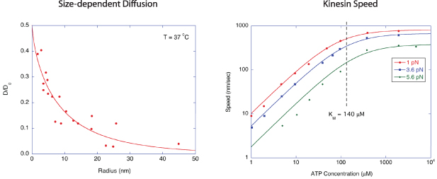
Figure 8. (a) Reduced diffusion coefficient relative to saline for particles in living fibroblasts, neurons and myotubes as a function of particle radius. (b) Speed of kinesin as a function of ATP concentration under three different loads. At low load, the speed saturates near 1 μm s−1.
Download figure:
Standard image High-resolution imageThe transport of small molecules inside living cells primarily is driven thermally as Brownian motion rather than through active transport, although molecular diffusion is also typically anomalous. Molecular transport can be measured using fluorescence correlation spectroscopy (FCS) [192, 193]. FCS probes fluorescent molecules that diffuse into and out of a small focal volume of an excitation laser. The residence time for a single fluorophore is related to the mean-squared displacement (MSD) of the molecule relative to the transverse focal width. The correlation times of the detected fluorescence intensity fluctuations are directly related to the residence times. FCS has been used to detect molecular diffusion in the cytoplasm [194], the nucleoplasm [195] and molecular diffusion within membrane layers [196]. The diffusion is usually anomalous [197] and can elucidate possible fractal geometry of intracellular structures [198]. Typical correlation times range from 10 ms down to microseconds, relating to characteristic frequencies of 100 Hz–MHz.
3.2. Molecular motors
Molecular motors within the cells provide the forces that cause persistent transport. Motors come in many types [3, 199]. These include molecular motors that move on the cytoskeleton, such as myosin on actin [26, 27], and kinesin and dynein on microtubules [24]. A distributed form of motor is cytoskeletal polymerization, as cytoskeletal filaments exert forces through extension supported by polymerization [200, 201]. In addition, rotary motors are anchored on the cell membrane, including ATP synthase as well as flagellar motors [202]. Nucleic acid motors are common, involving molecules that translate along DNA such as the RNA and DNA polymerases [33]. In these cases, molecules carrying chemical energy, such as ATP or GTP, as well as chemical or potential gradients, are converted into useful and directed motion in the cell.
Examples of motors, the forces applied, distances or times traveled, and speeds are given in table 2 for several types of motor processes discussed in the literature. The fifth column shows the product of Doppler frequency and persistence time, or the product of momentum change and persistence length. These products are equivalent and are equal to the Doppler number associated with that transport process (see section 4.3). Most of the motors are processive, meaning that they persist in a direction for a number of steps before changing direction or speed. For example, after a characteristic duration of 100 steps the kinesin motor is released from the microtubule [5]. This represents a persistence length of 800 nm and a persistence time of 0.4 s at a speed around 2 μm s−1. In every step, one ATP molecule gets hydrolyzed releasing about 20 kBT of free energy. The force that this release of energy can exert over the 8 nm step length is about 5 pN (assuming 50% efficiency [6]).
Table 2. Molecular motor speeds, Doppler frequencies and persistence.
| Motor or polymerization | Speed | Doppler frequency | Distance or time |
 or or 
| References |
|---|---|---|---|---|---|
| Kinesin | 2 μm s−1 | 6 Hz | [203] | ||
| Kinesin | 1 μm s−1 | 3 Hz | 15 | [5] | |
| Kinesin | 800 nm s−1 | 2.7 Hz | [191, 204] | ||
| Kinesin | 1 μm s−1 | 3 Hz | 10 s | 200 | [205] |
| Kinesin | 1 μm | 20 | [206] | ||
| Kinesin | 1 μm s−1 | 3 Hz | 600 nm | 10 | [207] |
| Kinesin/Dynein | 800 nm s−1 | 2.7 Hz | 100 nm–300 nm | 2–6 | [208] |
| Dynein/Dynactin | 2 μm s−1 | 6 Hz | [203] | ||
| Myosin V | 20 nm s−1 | 0.06 Hz | 1 μm | 20 | [26] |
| Myosin V | 300 nm s−1 | 1 Hz | 1.6 μm | 30 | [27] |
| ParA/ParB | 100 nm s−1 | 0.3 Hz | 2 μm | 40 | [209] |
| Actin network polymerization | 5 nm s−1 | 0.02 Hz | [201] | ||
| Tubulin polymerization | 20 nm s−1–300 nm s−1 | 0.07–1 Hz | 300 s | 15–100 | [200] |
| Filapodia extending | 40 nm s−1 | 0.12 Hz | 130 s | 100 | [210] |
| Filapodia retracting | 10 nm s−1 | 0.03 Hz | 100 s | 20 | [210] |
| WAVE complex | 70 nm s−1 | 30 s | [211] |
The most important molecular motors involved in intracellular transport are the kinesin and dynein superfamily proteins [24]. The kinesins consist of approximately 14 families of related proteins comprising approximately 50 different kinesin molecules in human cells. The dyneins are divided into two classes: cytoplasmic and axonemal. Both kinesins and dyneins are large macromolecules with molecular weights of 400 kDa and 1.5 MDa, respectively. Kinesins move towards the plus end of a microtubule carrying intracellular vesicles. In contrast, dyneins are motor proteins that move toward the minus end of a microtubule. Both execute processive motion of approximately 8 nm steps per hydrolyzed ATP. Large molecules synthesized in the cell body and intracellular components such as vesicles and organelles are too large to diffuse to their destinations through the crowded cytosol and hence must be transported by molecular motors along the cytoskeleton, primarily on the microtubules. Cytoplasmic dynein helps position the Golgi complex and other organelles in the cell, and helps transport vesicles, endosomes, and lysosomes, as well as the movement of chromosomes, positioning the mitotic spindles for cell division. Axonemal dynein is involved in the motion of cilia and flagella and is found only in cells that have those structures.
The speeds of kinesin and dynein are both in the range of 1.5 μm s−1 for single molecules at saturated ATP concentrations above 0.1 mM, although higher speeds are possible when multiple motors work in concert [203]. The kinesin stall force is weakly dependent on the ATP concentration and is typically around 7 pN [191] with similar values for dynein [212], although stall forces appear to be additive when multiple motors are involved [213]. Under a load of 5.6 pN, the velocity of a single motor saturates to 400 nm s−1 at an ATP concentration of 300 μM [191] shown in figure 8(b).
3.3. Vesicle and organelle transport
While molecular motors are too small to scatter light significantly, cytoskeletal motors move organelles or vesicles that do scatter sufficient light. The molecular motors produce speeds in the range of microns per second for vesicle and organelle transport. A simple application of Stoke's drag law provides a crude estimate for the stall force,

For an effective viscosity 300 times greater than water η = 0.3 Pa·s, for a spherical organelle of radius a = 1 μm and a speed of v = 1 μm s−1, the stall force would be 6 pN, which is roughly consistent with measured values [191, 212].
Among the smallest organelles are endocytic organelles which are also the fastest with speeds measured up to 8 μm s−1 and mean speeds in the range of 2 μm s−1 [175]. The dynamics of endocytosis are complex, and the initiation is associated with actin-mediated membrane dynamics [214, 215]. During transport, there can be coordinated motion at high speeds [216, 217], or bidirectional motion caused by antagonistic 'tug-of-war' mechanisms between kinesin and dynein [208, 218]. Lysosomes are a common type of intracellular vesicle with several hundred occurring per cell and varying in size from 0.1 to 1 μm in diameter. Because of the nature of their intra-vesicle materials, they tend to have high refractive index contrast relative to the cytosol and contribute significantly to light scatter [219, 220]. Lysosome speeds are in the range of half a micron per second and have speed PDFs that are monotonically decreasing. Motionless lysosomes are the most probable, and the standard deviation in speed is approximately equal to the mean speed [221], which is consistent with a decaying exponential probability distribution.
Mitochondria are ubiquitous organelles with several thousand mitochondria per cell and contribute significantly to light scattering from cells and tissues [220, 222]. Mitochondria move with a distribution of speeds [223]. Mean mitochondrial speeds range from hundreds of nanometers per second down to tens of nanometers per second. Finite persistence times of the mitochondrial displacements produce speed distributions that depend on observation time, and longer observation times generate lower mean speeds [224] because during long observation times some of the mitochondria in the initial test cohort stop or reverse. The mean speed scales approximately with the square root of the observation time for times around 1 s. The speed PDFs of mitochondria are generally monotonic decreasing as a function of speed with stationary mitochondria being the most probable [225], but with relatively long tails with high speeds up to several microns per second.
At the other end of the size scale from vesicles and mitochondria is the nucleus, which is one of the largest organelles in the cell. Therefore, nuclear speeds set the low-frequency behavior of intracellular organelle transport. As with all organelles, the distribution function of nuclear speeds is broad with the peak at zero speed, producing static light scattering as the dominant effect of the nucleus. The highest speeds for nuclei are around 300 nm s−1 which occur in bursts of several seconds with waiting times between bursts of about a minute [226]. The persistence length of nuclear transport is typically about one nuclear diameter, or about 5 μm [227, 228], and the motion is driven by the cytoskeleton [227, 229, 230]. The highest speeds produce Doppler frequency shifts up to 1 Hz, but these are rare, and the majority of the Doppler frequencies associated with nuclear transport processes are below 100 mHz [231]. The persistence lengths place the DLS firmly in the Doppler regime for the fastest motions. In addition to translation, nuclei also rotate with angular speeds of ten degrees per minute [232]. Drugs that affect nuclear motions include blebbistatin that inhibits myosin II and increases nuclear speeds by approximately 60% [233], while nocodazole inhibits microtubule polymerization and decreases nuclear speeds by a factor of two [232].
3.4. Cytoskeletal restructuring and active matter
The cytoskeleton is a dynamic and adaptive structure whose components—cytoskeletal elements and regulatory proteins—are in constant flux [37]. The cytoskeleton has several functions. It organizes the structure and contents of the cell, it connects the cell chemically and physically to the external environment, and it drives cell shape changes and cell movement associated with developmental biology as well as metastatic migration. The cytoskeleton is also part of the signaling functions of a cell through the process of mechano-transduction [90] as a cell senses its force and adhesion environment, triggering changes in internal signaling pathways that in turn lead to dynamic changes in cellular processes and motions.
Microtubules grow and relax through polymerization and depolymerization episodes known as treadmilling. Growth speeds can be up to 45 tubulin dimers (8 nm size) per second or up to 300 nm s−1 [234, 235]. The microtubules execute random walks during growth with persistence lengths of about 30 μm [236] which places this process well within the Doppler regime. The depolymerization rate can be much faster at 1000 dimers per second [234]. These speeds are in the same range as the fastest molecular motors and their organelle cargos. However, the microtubules are small with a 25 nm diameter, and even long filaments produce little light scattering by themselves. The microtubules exert forces on larger intracellular constituents that scatter light, but the load force slows down polymerization speeds [200]. Therefore, intracellular objects that move via interaction with microtubule forces are restricted to lower speeds with maximum speeds up to about 300 nm s−1 for a maximum Doppler frequency shift (under the standard optical configuration) of 1 Hz.
Actin filaments similarly grow through polymerization punctuated by shrinkage. Actin polymerization rates are typically 4 subunits per second for 370 subunits per micron [237] under normal monomer concentrations. This is a growth speed of about 10 nm s−1 and a Doppler frequency shift of 30 mHz. The speed decreases under load [201]. At high monomer concentrations the speed can be as large as 30 subunits per second for a speed of 80 nm s−1 and a Doppler frequency shift of 0.24 Hz. The shrinkage speeds can be much higher up to 0.6 μm s−1 and as high as 3 μm s−1, and the typical length of actin filaments is 1.5 μm [238]. Therefore, active actin polymerization in cells generates motions of cellular components with maximum speeds below 100 nm s−1 and Doppler frequency shifts below 300 mHz.
Biological matter is active matter [168, 239–241] driven by energetic processes that are far from thermal equilibrium with a direct connection to active gels [169] and their relationship to living systems [170]. The cell is composed of subsystems that, though interconnected, are themselves systems of active matter. The cytoskeleton is a highly active sub-system that experiences large fluctuations through polymerization and depolymerization driven by GTP. When combined with molecular motors such as myosin driven by ATP, this system represents an active gel [169] that shares similarities with liquid crystals [242, 243]. The plasma membrane, in addition to being driven by the cytoskeleton, also reacts to the forces of ion pumps and behaves as an active fluid film [244–247]. Another active subsystem is chromatin that experiences active reconfigurations during transcription [248]. In addition to subsystems, there are also macro-systems that behave as active matter, such as organized tissue [169]. Force fluctuations are linked to velocity fluctuations, which in turn are linked to MSDs. This provides an avenue for analyzing the active processes that occur within cells [249, 250].
Active processes and materials can have steady-state behavior that represents a dynamic equilibrium that stands in for thermal equilibrium. Some of the results of equilibrium thermodynamics can be applied in this case, but with a reinterpretation of the parameters in terms of effective properties, such as effective temperatures that have functional dependence on characteristic scales (time scales and spatial scales). Effective temperatures of biological processes can be orders of magnitude larger than actual thermal temperatures, leading to dynamic properties that are much larger than thermal effects. For instance, transport by active processes may be characterized as random walks, but with MSDs much larger than possible with thermal Brownian motion. As an example, the effective temperature of a normal cell, versus one that was ATP depleted, show markedly different effective temperatures [251] when beads were bound to the actin cortex through membrane receptors. Active actin-myosin gels [252] driven by molecular motors and cytoskeletal filaments violate the fluctuation-dissipation theorem. At frequencies decreasing below 1 Hz the effective temperature increases, corresponding to larger MSDs from slow large-scale membrane and cell motions. The effective temperature increases approximately as 1/ω2 reflecting the increase in active stress fluctuations [252, 253].
3.5. Membrane dynamics
The dynamics of cell membranes is one of the most important contributors to DLS in living tissue. The fraction of the cell volume made up of the lipid membrane layers is small, but the membrane is an envelope that coordinates the motions of all the internal constituents [144]. Motions of a region of the cell membrane are accompanied by coordinated motions of all the internal components near that region. Membrane motions in living tissue are dominated by active processes driven by the connection of the cytoskeleton to the membrane at focal adhesions [38]. Therefore, active membrane dynamics and associated speeds and persistence times are strongly related to cytoskeletal speeds and persistence times.
Transverse spatial modulation in the membrane can be characterized by a spatial frequency k = 2π/λ, where λ is the characteristic length of a section of persistent curvature. For instance, thermal excitations of passive membranes (when there are no active processes) cause membrane modulation, called flicker, in erythrocytes [180, 254–256]. The principle of equipartition of thermal energy gives the thermal MSD as
where A is the membrane area, γ0 is the tension, and κb is the membrane bending stiffness. The mean-squared membrane displacement is proportional to the physical temperature, but inversely proportional to the area of the membrane. The fluctuations are largest for the smallest spatial frequencies, with a long-wavelength cutoff of the spatial frequency k given by  where d is the diameter of the cell. The relaxation rate for a membrane undulation with spatial frequency k is given by [257]
where the viscosity η pertains to fluid redistribution within the cell [190]. However, in the active fluctuations of membranes, such thermal forces are dwarfed by energetic processes that are far from thermal equilibrium [247]. Membrane fluctuations have ATP dependence [258], signifying the requirement for energy to drive the active processes, and effective temperatures related to MSDs are much larger than the temperatures of the thermal bath [259]. Therefore, the membrane fluctuations are dynamic processes with characteristic lengths, amplitudes and relaxation times [260] that contribute to DLS from living tissue.
The speeds of membrane motions are comparable to speeds of cytoskeletal restructuring [261]. For instance, filopodium have repetitive cycles of elongation and persistence that depends on actin crosslinkers with characteristic displacements of microns in minutes [210]. A displacement of 2 μm in one minute is a speed of 30 nm s−1 which produces a Doppler frequency shift of 100 mHz in the standard configuration.
Mitosis is a key energetic process in actively proliferating tissue [44], as in developing embryos, in tissue culture grown from immortalized cell lines and in natural cancer tissues. The duration of the different phases of mitosis are approximately half an hour for prophase, 2–10 min for metaphase, 2–3 min for anaphase, 3–12 min for telephase, and a fairly long duration for reconstruction ranging up to 2 h. The entire mitotic process can take between an hour and three hours, depending on the cell type and conditions. Chromosome separation in preparation for cell division is relatively slow at 15 nm s−1 [262] (50 mHz in the standard configuration). However, contractile ring speeds during cytokinesis are relatively faster at around 100 nm s−1 (0.3 Hz in the standard configuration) with long persistence times of hundreds of seconds [263].
3.6. Cell crawling and metastasis
Cellular motility is a central characteristic of living matter. The motion of cells through three-dimensional tissue supports fundamental processes such as the formation of tissues and organs during embryonic development, wound healing, infiltrating immune response and cancer metastasis [264]. The central player in cell migration is the cytoskeleton composed of microtubules, actin filaments and intermediate filaments. Actin plays a particularly active role by using polymerization/depolymerization forces to reshape the cell while providing traction and hydrodynamic forces [265]. The most common migratory cell types that have been studied are keratocytes (from fish scales), fibroblasts, leukocytes (neutrophils) and metastatic cells. The maximum speeds of these migratory cells vary over three orders of magnitude from microns per hour to millimeters per hour, corresponding to standard-configuration Doppler frequency shifts from 1 mHz to 1 Hz, respectively. For instance, keratocytes and wound-healing cells in the cornea are among the fastest cells crawling with speeds of tens of microns per minute (standard-configuration Doppler shift of 1 Hz). However, many common migratory cell types, including many cancer cell lines, travel with maximum speeds of tens of microns per hour (standard-configuration Doppler shift of 25 mHz) [266].
The majority of studies of cell motion have been performed in 2D formats [267] because of the ease of culturing and imaging, but more recently the focus has shifted to imaging in 3D matrices because of its greater physiological relevance [268]. The migration of cells in 3D can be studied using selective plane illumination microscopy (SPIM) [269–271]. Speeds through 3D matrices tend to be smaller than under equivalent conditions in 2D depending on the size of pores [272, 273] in the collagen gels, the orientation of the fibrils [274], and cellular density [275], but the motions tend to be more persistent [276] than in 2D.
The large cross-sectional area of cells migrating through tissues represents an extreme limit to biological motion through constrained geometries. The forces driving the motion can be relatively large by combining the forces from numerous focal adhesions with persistent orientation, but the geometric constraints produce large effective viscosity that yields very low speeds and very low standard-configuration Doppler frequencies in the range between 1 mHz and 10 mHz for many types of migrating cells. These low frequencies are currently at the low end of interferometric stability which is dominated by 1/f noise. On the other hand, the high light scattering from cell membranes and the high number density of light scattering objects in dense tissue driven by active forces of the cytoskeleton with high effective temperatures leads to a biological signal at these low frequencies that can be comparable to or larger than the 1/f noise contribution. Therefore, cell motility, including metastatic motions through tissue, can contribute to the fluctuation power spectrum measurable above the noise floor in interferometric and holographic light scattering apparatus [277].
4. Intracellular transport: mathematical models and light scattering
All biological processes have stochastic contributions to their dynamics. Intracellular thermal Brownian motion of small molecules lies at one extreme that is ideally stochastic. Cytokinesis lies at the other extreme in which the motion during cell division is directed and deterministic. Most biological processes lie between these extremes having both stochastic and deterministic contributions to motion. For instance, vesicle and organelle transport is processive with persistent motion, as one or more molecular motors carry them along cytoskeletal tracks. But the motors stochastically detach and reattach, causing the objects to falter or change direction. Similarly, the active motion of the cell membrane is driven by successive growth and collapse of cytoskeletal filaments, causing persistence in the motion, but superposed with stochastic fluctuations. The mixture of deterministic motion with stochastic motion opens a wide variety of possible intracellular transport models that attempt to capture the essential behavior of subcellular systems.
Stochastic processes in biology draw from a broad range of probability distributions. The chief distinction in these distributions is whether they satisfy the central limit theorem with finite moments, or if they have divergent tails that do not obey the central limit theorem and have (some) moments that are undefined [278]. Poissonian, Laplacian and Gaussian distributions are examples of well-behaved distributions that satisfy the central limit theorem. Conversely, the common Cauchy distribution (also known as the Lorentzian lineshape) has a divergent first moment, as do other Levy-stable distributions [278]. The power-law Pareto distribution, being self-similar, fails to have any finite moments. Transport processes that are governed by well-behaved probability distributions are called regular transport, while those governed by power-law distributions are among anomalous transport processes. Both types of stochastic transport yield random walks.
4.1. Regular transport models
Regular transport is represented by conventional transport processes such as steady motion (drift) and random-walk motion (diffusion), with transport parameters characterized by probability distributions with well-defined moments, such as Gaussian or Laplacian. Regular transport processes in cellular media provide the first level of approximation towards understanding experimental results, yielding estimates for characteristic transport lengths and times and hence are useful for understanding the generally anomalous scaling of length and time in cellular processes.
Regular transport is associated with MSD that is a polynomial function of time within limiting regimes of behavior. Examples are illustrated in figure 9 for ballistic transport, persistent walks and Brownian motion. The MSD increases quadratically as t2 for ballistic transport and linearly as t for Brownian motion. The intermediate regime is characterized by a cross-over time (or cross-over length) between one limit and the other. Whether a transport process is considered ballistic or diffusive depends on the observation time scale. For instance, in the ballistic limit the persistence time is longer than the observation lag time between measurements, while in the Brownian limit the persistence time is much smaller than the time lag between measurements and the transport converges in the limit to a Wiener process. Hence, characterizing transport as ballistic or diffusive is not an intrinsic behavior but is observation time-scale dependent. If there is an additional measurement scale, such as the wavelength of light, then ballistic or diffusive transport can be defined by the relation between the persistence length and the wavelength. This is the case for Doppler light scattering.
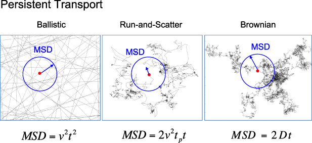
Figure 9. Regular transport varies smoothly from the ballistic limit (with long persistence times) to the Brownian limit (with vanishing persistence times). The mean-squared displacement (MSD) is polynomial in time. In the intermediate regime of run-and-scatter, the mean-squared speed is v2 and the mean persistence time is tp.
Download figure:
Standard image High-resolution image4.1.1. Brownian diffusion.
Conventional Brownian diffusion is governed by the DE for the PDF as
where D is the diffusion coefficient. The PDF is
where W(x,t) is also called the propagator. The Fourier transform of the DE is
where the Fourier components experience simple exponential decay

and W(q,t) is the time-dependent characteristic function of the probability distribution. The temporal Fourier transform of the characteristic function is
which represents a Lorentzian line shape spectrum. In light scattering, the characteristic function W(q,t) plays the central role defining the light-scattering autocorrelation function, and its temporal Fourier transform W(q,ω) plays the central role defining the fluctuation power spectrum of a dynamic target. In many of the sections that follow, it may be convenient to describe processes either in terms of W(q,t) or W(q,ω), and sometimes W(q,s) (a Laplace transform), depending on the circumstances.
4.1.2. Wiener process.
A Wiener process (named after Norbert Wiener) is the limiting behavior of a random walk as the step size decreases to zero and the number of steps increases to infinity. A Wiener process yields a continuous curve whose derivatives exist nowhere. Consider a random variable that executes drift and random walk

The differential dw is the differential of a Wiener process and can be written explicitly as

where N(0,1) is a normal probability distribution with zero mean and unit variance. The differential in the square root guarantees the following time-average properties of the Wiener differential
The square-root of the differential makes equation (4.7) a stochastic differential equation (SDE). The solution of this SDE is

where the MSD = b2 t. This is the classic Brownian motion first derived by Einstein in 1905 [279].
Einstein neglected inertia in his derivation in his stochastic Brownian motion analysis that he expressed in terms of stochastic displacement neglecting forces. However, there are systems for which inertia does play a role, at least at short times, as well as persistent systems that are not in equilibrium and behave as if they had inertia during their runs. For these systems, a more complete approach is that of Langevin in 1908 [280] that explicitly includes force terms in the velocity SDE. The solution of this SDE is known as the Ornstein–Uhlenbeck (OU) process, explored by Ornstein and Uhlenbeck in 1930 [281] who expanded on Langevin's work. The original OU velocity process was applied to stochastic transport in gases under thermal equilibrium, but it also can be a mathematical analog for active and persistent transport far from equilibrium, as in living systems.
4.1.3. Ornstein–Uhlenbeck (OU) process.
The OU process contributes a stochastic velocity fluctuation to the usual damped motion. The stochastic contribution to the velocity has the form

This SDE represents a decaying exponential with decay rate γ modified by a fluctuation term with amplitude Γ. This expression can apply to the case of viscous damping where −γv is the drag force. The solution for the average velocity is

and the variance is [282]
The speed PDF for the OU process is
and this speed distribution generates the autocorrelation function
for an exponentially damped Doppler frequency shift.
The long-term limiting value for the variance is
which defines the parameter Γ to be

Equation (4.15) is analogous to the fluctuation-dissipation expression for a system in equilibrium but expressed in terms of the persistent speed v0 instead of temperature. As an estimate of Γ, for a speed of 1 μm s−1 and a persistence time of 1 s (appropriate for organelle transport), then Γ2 = 2 Hz·μm2 s−2. As an alternative approach to estimating Γ, if the transport processes were viewed in steady state, then this long-term expression would be related to a form of the equipartition theorem in which forces and velocities provide the underlying energetics for intracellular motions and are also the source of the fluctuations. The power provided by intracellular forces at low Reynold's number is
where  is the average power provided by active transport. This gives, assuming steady state holds, the relation
where the average power is provided by molecular motors driven by energetic hydrolysis of ATP for molecular motors, or GTP for cytoskeletal restructuring. As an estimate, consider a persistence time of 1 s and a vesicle of radius 1 μm being transported by a single molecular motor moving at 1 μm s−1. If the motor force is approximately 2 pN and the effective viscosity is 1 Pa·s, this also yields a value of Γ2 = 2 Hz·μm2 s−2 comparable to the estimate from the fluctuation-dissipation theorem, although the wide range of particle sizes and effective viscosities produce a similarly wide range of values for Γ for different types of intracellular processes.
4.2. Single-scattering limit of DLS
The single-scattering limit of DLS is the limit of optically thin, or highly dilute, samples. Although light transport in living tissue is highly scattering, the typically large anisotropy factors of g ≈ 0.9 favor small-angle forward scattering. The mean free length before large-angle scattering of a photon is roughly 100 μm in tightly-packed cells of epithelial tissue, although this is only a rough estimate and actual numbers can vary significantly depending on the tissue type. Therefore, shallow penetration of light into tissue up to approximately 100 μm leads to roughly a single high-angle scattering event. Only the large-angle events carry significant Doppler frequency shifts, hence shallow light scattering even up to a few hundred microns remains mainly in the single-scattering regime. Expressions for field or intensity autocorrelation functions are readily obtained in the single-scattering regime because they are simple sums (or integrals) over partial waves. Although the results in this section pertain to light scattering up to about several hundred microns inside tissue, the transition to multiple scattering keeps the same qualitative trends but with higher characteristic frequencies because of the compounded phase excursions of multiple scattering.
For 3D diffusion from a Wiener process, the probability functional is
which gives the diffusion field autocorrelation function

and intensity autocorrelation function
On the other hand, for a 3D Gaussian distribution of ballistic velocities, the probability functional is
which gives the field autocorrelation function

and the intensity autocorrelation function
In addition, if the scattering objects experience a uniform drift in fixed direction, the probability functional is

which gives the drift autocorrelation function

where the cosine term is equivalent to a Doppler beat frequency. The intensity autocorrelation is
As described in sections 2 and 3, persistent flights along isotropically-oriented filaments or microtubules are driven by molecular motors that run at approximately constant speeds in essentially one-dimensional segments (persistence lengths) that are isotropically oriented. Isotropically-averaged 1D transport does not yield the same autocorrelation functions as 3D transport. For instance, the distribution function for one dimensional isotropic motion is given by equation (4.18) [283]. The associated intensity autocorrelation function when averaged over all angles is
The intensity autocorrelation function equation (4.27) is much different than the simple exponential of equation (4.19). The autocorrelation function behaves as an error function with the same characteristic time  as 3D diffusion, but the functional dependence is different. DLS fluctuation spectra from 3D diffusion has a classic low-frequency plateau and a knee frequency above which the spectral density falls as 1/ω2. But applying the Wiener–Khinchine theorem to equation (4.27) does not produce a low-frequency plateau but yields instead a 1/ωa behavior. This makes the characteristic knee in the spectrum less distinguishable because the spectral power switches from one power law to another.
For long persistence times, the three-dimensional ballistic transport model is the same as averaging 1D transport over all angles. For a displacement  , the distribution function is

and the intensity autocorrelation function is
The oscillatory sinc function arises from the Doppler frequency. The associated homodyne spectral density is
where  is the triangular function. The spectra from isotropically-averaged 1D diffusion to 3D diffusion are compared in figure 10 relative to the ballistic Doppler edge.
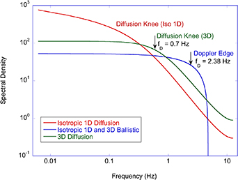
Figure 10. Spectral power density for isotropically-averaged 1D diffusion compared to 3D diffusion. Also shown is the Doppler edge for ballistic transport. Results are averaged isotropically over all angles. A diffusion coefficient is used for the first two cases with D = 0.01 μ2 s−1, and a uniform velocity v0 = 1 μm s−1 is applied to the ballistic case.
Download figure:
Standard image High-resolution image4.3. Lifetime broadened Doppler
When coherent light scatters from a uniformly moving object, the phase of the scattered light changes linearly with time. When this interferes with a stationary reference wave in the interferometer, the intensity modulation is sinusoidal in time, persisting for as long as the particle's persistence time. For one-dimensional motion with uniform speed, particle motion changes through a reversal of the velocity vector, and the detected sinusoidal intensity undergoes time reversal. Therefore, the interferometric time series is mathematically equivalent to an ensemble of undamped, randomly time-reversed harmonic oscillators.
The differential change in velocity of a moving particle under a random time reversal is
where tp is the mean persistence time, assumed to be decaying exponentially distributed. In this case, the equation describes an ensemble of particles, known as the persistent random walk model [276]. The average velocity distribution is

and variance
The mean speed of the randomly time-reversing ensemble decays exponentially with a time constant τ = tp/2 which is a dephasing time like the T2 time of photon echoes or NMR. The ensemble average is equivalent to a damped harmonic oscillator with a time constant τ = 1/γ where the equivalent damping coefficient is

The homodyne spectral power density of fluctuations for a damped harmonic oscillator is
The interferometric detection of randomly time-reversed steady motions differs mathematically from lifetime broadening. For a constant sinusoidal emission that experiences random phase jumps, the subsequent phase is uncorrelated to the preceding phase. This simplifies the mathematical description, and lifetime broadening leads to a classic Lorentzian line-shape with a linewidth determined by the time-frequency uncertainty product of Fourier analysis (analogous to the Heisenberg uncertainty principle). The time reversal waveform in the time-reversed case is continuous everywhere, while the random phase jump waveform has discontinuous jumps. The stochastic phase jumps produce larger discontinuities in the waveform, producing wider bandwidth relative to stochastic time reversals. The asymptotic behavior of both cases (at high and low frequencies) are the same. The one-dimensional Doppler broadening for stochastic time reversal is shown in figure 11 compared to random phase jumps.

Figure 11. Comparison of time reversal events versus phase jump events in the back-scattered field. (a) Time-dependent field for time reversal and phase jumps. (b) Resulting 1D heterodyne power spectra. The parameters are fD = 0.3 Hz, tp = 10 s and ND = 18.
Download figure:
Standard image High-resolution imageThe Doppler frequency shift  and the persistence time
  (and equivalently the momentum transfer
  and the mean free path
  ) define a dimensionless scaling parameter called the Doppler number, ND, given by

When ND = 1, then
sets a characteristic persistence length Lp relative to the reduced wavelength λred. For a refractive index  and a free-space wavelength
From the perspective of light scattering, the dividing line in living tissue between diffusive transport and Doppler (ballistic) transport occurs when the mean-free transport paths of the intracellular process is approximately 50 nm. The conditions on the Doppler number ND define different regimes where Doppler effects dominate the light scattering when ND is much greater than unity, and diffusive light-scattering character (diffusive knee) occurs when ND is much smaller than unity, with cross-over behavior between the two regimes around ND ≈ 1. Most active transport processes in cells have long mean-free paths that place DLS in living tissues in the Doppler regime (see table 2). However, because of the overlapping of many different transport processes with different characteristic speeds, the Doppler edges are distributed across a broad frequency range, and the spectral power densities from most tissues appears diffusive without distinct Doppler edges.
Examples of the Doppler spectrum for uniform velocity and finite persistence time is shown for 1D transport in figure 12 for the Doppler number ranging from 10 to 0.1 for a fixed Doppler frequency fDopp = 1 Hz. In the diffusion regime (ωτ = 0.1) the diffusion knee occurs at fDiffus = q2 D/2π where the diffusion constant is D = v0 2 τ, and the spectral fall-off above the knee is 1/ω2. There is a peak in the Doppler regime (ωτ = 10). The spectral fall-off above the peak in this regime is much steeper than the 1/ω2 slope of a diffusion lineshape, which is one signature of the Doppler regime.
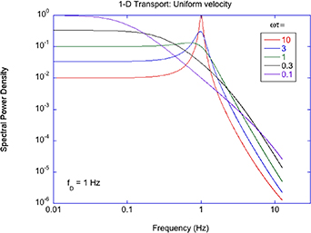
Figure 12. Heterodyne Doppler spectral power densities as function of frequency for one-dimensional motion for a Doppler frequency of 1 Hz. The ωt product ranges from 10 (Doppler regime) to 0.1 (diffusion regime).
Download figure:
Standard image High-resolution imageIn isotropic tissue, the one-dimensional transport is distributed uniformly with angles

For constant-speed scattering objects, the contribution to the fluctuation power spectrum is
In isotropic tissue, the total power spectrum is integrated over all Doppler frequencies
Examples of isotropically-averaged 1D motion are shown in figure 13 for Doppler numbers ND = 0.1, 1, and 10 [277]. The dashed curves are for 1D motion, showing a clear Doppler peak at  for
for  . In the case for
  , there is a diffusion knee at
  . The cross-over in behavior from a Doppler peak to a broad spectrum occurs around
  . Averaging over all angles removes the peak at the Doppler frequency, even in the case of large ND, although there is a distinct edge at the Doppler frequency for this case. When the Doppler number is small, a diffusive knee structure emerges at lower frequencies, but there is no low-frequency plateau as occurs for isotropic 3D diffusion.

Figure 13. Spectral power density plotted against frequency for comparison of unidirectional (dashed) versus isotropically averaged 1D (solid) power spectra for ND = 0.1, 1, and 10. [Reprinted/Adapted] with permission from Li et al [277] © The Optical Society.
Download figure:
Standard image High-resolution imageThe cross-over behavior from the Doppler regime to the diffusion regime is described in terms of a knee frequency, which is a function of diffusion and ballistic frequencies and persistence time through
For long persistence times  , the knee frequency is a Doppler edge at the Doppler frequency ωD, while for short persistence times, the knee frequency is the diffusive frequency
  [277].
4.4. Continuous time random walk (CTRW)
A heuristically simple model for a broad range of transport processes, including both regular and anomalous transport, is the CTRW [284] with constant speed [285, 286]. The original model assumed discontinuous jumps which aided theoretical descriptions, but it is not a physically relevant model of actual motion. The current review treats only the modified CTRW model where the particles move with constant speed between rests as shown in figure 14. The length of the walk between stops is the persistence length, and because of the constant speed between stops, the persistence length is coupled directly to the persistence time. The persistence length is drawn from a specified distribution that may have finite moments (normal transport) or moments that diverge (anomalous transport). The resting times at each stop also are drawn from a specified distribution that may be different than that for the persistence length. Therefore, this transport model is governed by two PDFs: one for the persistence time and one for the resting time. This type of transport model can have simple microscopic interpretations. For instance, a transport process may have a spatial distribution of traps that temporarily bind a walking object. If the object is a particle, the trap may be a local potential well with a probability per time that the particle will escape. Or the transporting object may be an organelle or vesicle that detaches from a molecular motor and waits for another motor to bind it.
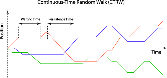
Figure 14. Continuous-time random walk (CTRW) model with constant speed between resting times. The resting times and persistence times are drawn as random samples from underlying probability distributions that may have finite (normal transport) or divergent (anomalous transport) moments.
Download figure:
Standard image High-resolution imageIf both the resting times and walk lengths are drawn from distributions that have finite first and second moments, then normal transport occurs. However, if one of the distributions does not obey the central limit theorem, then anomalous transport is the result. The anomalous transport can be either subdiffusive or superdiffusive. If the walk lengths have finite moments, but the resting times have divergent moments, then the transport is subdiffusive. Conversely, if the resting times have finite moments, but the walk lengths have divergent moments, then the transport is superdiffusive. If both path length and resting time have divergent moments, then there is a complicated balance between superdiffusive and subdiffusive behavior.
The CTRW transport model can be one-dimensional, for which the direction after de-trapping can be in the original or the opposite direction. Or the transport can be two-dimensional or three-dimensional as the particle randomly chooses among orientations after de-trapping. The selection of orientations can be isotropic or anisotropic. Furthermore, the constant speeds can be sampled from a distribution of speeds. These different versions of the CTRW can be invoked to model different types of biological processes, including transporting vesicles and organelles, internal restructuring of the cytoskeleton, motions of the cell membrane, among others.
4.4.1. One-dimensional persistent walk with no resting time.
For a persistence time distribution  , the number of surviving walkers after a time t is
To couple the persistence time and persistence length, the position-time distribution function for the finite-speed walk has survival functions
where the delta function produces a ballistic peak in the distribution. While the main function of interest for light-scattering analysis is the propagator W(q,t) (the autocorrelation function) and the temporal Fourier transform W(q,ω) (the power spectrum), the most natural expression for the propagator in the CTRW is through the Fourier–Laplace transform W(q,s) because it uses the shift properties of the Laplace and Fourier transforms. Despite this advantage, even if the Laplace-transformed propagator W(q,s) can be derived analytically, the inverse Laplace transform may not be available analytically, and numerical inversion of Laplace transforms can be problematic.
The Laplace-transformed [278] no-resting-time propagator [287] is
where the Laplace-transformed survival function is
If the MSD of the persistence is finite, this leads to classical diffusion, but with a modification caused by the ballistic front that produces a Doppler peak in the power spectrum.
As an example of normal transport, consider the case for decaying exponentially-distributed persistence times and no resting time. The persistence time distribution and its Laplace transform are
The complex expression in terms of space-time coupling of the ballistic front is
The survival fraction is
and the inverse Laplace transform is
which is the decaying autocorrelation function of two delta functions moving at speeds ±v. The Fourier transform in this case is
which is a power spectrum with a Doppler peak at ωD = qv.
The CTRW model lends itself to straightforward numerical Monte Carlo simulations. The phases of the partial waves scattered from a collection of N particles, that are distributed in three dimensions, depend only on the detection direction relative to the transport direction and hence depend only on transport in one spatial dimension. The initial phases of the scattered fields are randomly selected, and the transport of N one-dimensional walkers proceeds according to the probability distributions of the CTRW model. The net scattered field is a linear superposition of individual scattered fields.
Monte Carlo examples are shown in figures 15 and 16 for 1D motion and a constant speed v0 = 300 nm s−1 with decaying exponentially distributed persistence times. The Doppler numbers in the two cases shown are ND = 0.3 and ND = 3 which are in the cross-over regime between ballistic and diffusive transport. The position distribution in figures 16(a) and (b) (on log position) for the lower Doppler number ND = 0.3 broadens diffusively over time. The case for figures 16(c) and (d) for higher Doppler number ND = 3 has a ballistic front at early times that converts into a diffusive front at later times. The RMS displacements as functions of lag time are shown in figure 17(a) for the two Doppler number cases. The RMS displacement is ballistic at short times and converts to diffusive at late times. The cross-over from ballistic to diffusive transport occurs later for the higher Doppler number case. The diffusive 1D transport for the lower Doppler number produces a fluctuation power spectrum that is diffusive for both the heterodyne and homodyne spectra, and the ballistic front for the higher Doppler number causes a broad Doppler peak in the power spectrum in figure 17(b). Higher Doppler numbers have sharper peaks in the 1D transport case.

Figure 15. Particle probability distribution function for constant 1D velocity at different times from 0.8 s to 80 s for v = 300 nm s−1. The 100 000 particles begin at t = 0 as a delta function. At early times there is a ballistic front, seen as the double peaks, and a scattered fraction seen as the values between the peaks. The ballistic fronts decay exponentially, and at late times convert to a broad diffusive background.
Download figure:
Standard image High-resolution image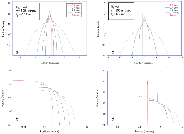
Figure 16. One-dimensional Monte Carlo particle distribution functions for v = 300 nm s−1 and Doppler numbers ND = 0.3 and 3 with decaying exponential persistence times. (a) Linear and (b) log position distribution for ND = 0.3 at successive times. (c) Linear and (d) log position distribution for ND = 3 at successive times. The ballistic front converts over time to a diffusive profile.
Download figure:
Standard image High-resolution image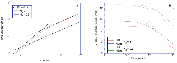
Figure 17. Effect of Doppler number for decaying exponential distribution of persistence in one-dimensional Monte Carlo simulations. (a) The RMS displacement versus time. Transport for higher Doppler number maintains ballistic behavior for longer times than for smaller Doppler numbers before becoming diffusive. (b) Spectral power densities versus frequency for one-dimensional transport for ND = 0.3 and 3 for heterodyne and homodyne spectra.
Download figure:
Standard image High-resolution imageThe Monte Carlo simulations for 1D transport are averaged isotropically to represent the situation inside isotropic living tissue. As discussed in section 2.2, most active transport inside tissue is isotropically-averaged 1D motion rather than 3D motion. The distinction is important, because the fluctuation power spectra for isotropically-averaged 1D transport are not equivalent to the spectra for isotropic 3D transport. The Monte Carlo simulations are extended to ensembles of 1D transport oriented at different angles relative to the light backscattering direction, and the power spectra are averaged. The results of a Monte Carlo simulation of isotropically-averaged 1D transport are shown in figure 18 for the ND = 3 case. The RMS displacement and power spectrum of the isotropically-averaged results are compared to the 1D case. The RMS displacements are reduced because of the additional degrees of freedom, but the transition from ballistic to diffusive behavior is not affected by the angular averaging. Doppler spectra are shown in figure 18(b). The Doppler 'peak' for 1D transport is converted by the angular averaging to a Doppler 'edge'. Higher Doppler numbers produce sharper edges. This Doppler edge is the dominant feature in experimental results to be shown in section 5. The knee frequency on the homodyne spectrum is equal to twice the knee frequency of the heterodyne spectrum.
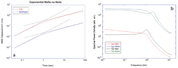
Figure 18. Isotropic Monte Carlo angular averaging over 1D oriented transport for v = 300 nm s−1 and tp = 0.5 s. (a) The RMS displacement as a function of lag time for 1D versus isotropically-averaged 1D transport for ND = 3. The RMS displacement after averaging is ten times smaller than the 1D value, but the break in scaling between ballistic and diffusive transport is retained. (b) Homodyne and heterodyne spectral power densities for 1D versus isotropically-averaged 1D transport for ND = 3. The isotropically-averaged Doppler 'peak' is converted to a Doppler 'knee'.
Download figure:
Standard image High-resolution imageChanges in intracellular transport, for instance caused by applied therapeutics or changing environmental conditions such as temperature or osmolarity or pH, have the largest effects on the edge feature in the power spectra similar to modulation spectroscopy in solid state physics [288]. An example simulation is shown in figure 19(a) for a Doppler edge with ND = 3 under a 30% decrease in transport speed. The differential change in figure 19(b) shows a dip at the Doppler frequency for the homodyne and heterodyne spectra. Modulation spectroscopy of the Doppler edge is an important technique in the study of pharmaceutical effects on living tissue described in section 5.

Figure 19. Example of isotropically averaged Doppler-edge spectroscopy for tp = 0.5 s and ND = 3. The transport speed decreases from 300 nm s−1 to 200 nm s−1. (a) Homodyne and heterodyne power spectra. (b) Log-difference of the Doppler edge spectra for homodyne and heterodyne.
Download figure:
Standard image High-resolution image4.4.2. One-dimensional persistent walks with rests.
Most biological transport is composed of persistent walks followed by rests. When the resting time distribution is  then the number of walkers remaining at rest after a time t is
and the propagator becomes [289]
As an example, for decaying exponential distributions of rest times
The propagator, even in this simple case, is not easily inverted. Monte Carlo simulations are shown in figure 20 for 1D transport and ND = 3 with a mean rest time tr = 0.5 s compared to no rest time. The extra rest time slows the transport and shifts the transport and power spectra to more diffusive behavior. The effect is particularly dramatic in the case of the power spectra. The 1D Doppler peak (for 1D transport) is broadened substantially by the extra rest time. The effective Doppler number in this case is reduced from the no-rest-time value to

Figure 20. Exponential persistence for v = 300 nm s−1 with persistence time tp = 0.5 s and rests for 1D transport. (a) The RMS displacement versus lag time for one-dimensional motion for two waiting times tw = 0 and 0.5 s. (b) Homodyne and heterodyne spectral power densities for one-dimensional motion. The extra wait time shifts the effective Doppler number to lower values, shifting the transport from ballistic to more diffusive.
Download figure:
Standard image High-resolution imageThe results in figure 20 are for one-dimensional transport. Isotropically-averaged transport further reduces the ballistic signatures in the power spectra into apparently diffusive spectra.
The trend towards apparent diffusive signatures of intracellular transport caused by multiple overlapping spectra is a common property of intracellular Doppler spectroscopy. Despite the relatively long persistence lengths of the intracellular constituents, which produce bare Doppler numbers exceeding unity, non-uniform transport with frequent rests produces linear MSD functions and apparent diffusive spectra without strong spectral signatures at the Doppler frequency. However, Doppler power spectra retain remnants of the Doppler edge, and small perturbations of the probability distributions associated with intracellular transport can produce subtle changes in the power spectra that can be interpreted in terms of changing transport parameters. Experimental observations of some of these effects will be discussed in section 5.
4.5. Anomalous transport
When the distribution functions Ψ(τ) and ρ(τ) for persistent transport and rests, respectively, have finite moments, they produce normal transport that transitions from ballistic to diffusive as the effective Doppler number decreases from greater than unity to less than unity. For Gaussian distributions, the MSD increases linearly with time, while in the ballistic case it increases as the square of time. Both of these limits are considered part of normal transport with a transition regime between the limits that is also part of normal transport. However, if one or both of Ψ or ρ have divergent low-order moments, then anomalous transport occurs. Anomalous transport has non-polynomial MSD, usually varying as a power law in time for short times [290–292], but extending over at least an order of magnitude, which distinguishes such scaling behavior from simple transitions between limits. The MSD in the scaling regime is
When δ > 1 the transport is called superdiffusive, and when δ < 1 the transport is called subdiffusive. When δ = 1 the transport is Brownian or diffusive. One of the simplest examples of anomalous random walks are drawn from Lévy stable probability distributions [134, 278, 292–294].
4.5.1. Levy stable distributions.
Probability distributions can have power-law behavior at large values of the argument, such as
which is called a heavy tail as the probability falls more slowly than exponentially. Heavy tails cause rare high-amplitude events known as outliers (and sometimes as 'black swans'). However, these events are fundamentally part of the distribution and can have a disproportionate effect on variances or mean values. These distributions include the so-called stable distributions for which a sum of two independent random variables sampled from a stable distribution have the same distribution. For instance, the sum of two Gaussian-distributed independent variables is also Gaussian distributed.
A probability distribution can be defined as the Fourier transform
of a function  known as the characteristic function of the probability distribution. The Lévy symmetric stable distribution is defined through a characteristic function as
which has the parameters α and γ, and the characteristic function is a stretched decaying exponential. The Lévy distribution has a power law tail given by equation (4.57), but has a characteristic length scale set by the parameter γ. The Fourier transform of the Levy distribution is simply the stretched decaying exponential characteristic function

This form comes in handy when considering light scattering from motile subcellular constituents displaying Levy distributions of mean free path.
The Levy stable distributions have several recognizable special cases. The special case of the Lévy distribution for α = 2 is a normal (Gaussian) distribution, and the special case of the Lévy distribution for α = 1 is the Cauchy distribution given by
The Cauchy distribution has a scale set by γ, but it has a divergent mean value, violating the central limit theorem. When a distribution satisfies the central limit theorem, increasing the number of samples from the distribution allows the mean value to converge on a finite value. However, for the Cauchy distribution, increasing the number of samples increases the chances of obtaining black swan events, which skews the mean value that diverges in the limit of an infinite number of samples.
Stable distributions with divergent moments are suspected to play roles in biology. For instance, a random walk with a Levy distribution of path lengths can be an efficient means for an organism to search for food [295, 296]. Similarly, Levy flights can participate in intracellular transport processes [297–299] and cell migration [300]. Resting times, as well as persistence lengths, can have stable distributions and may explain why anomalous transport occurs in intracellular motion. Examples of Levy stable PDFs are shown in figure 21 for a range between α = 1 (Cauchy) and α = 2 (Gaussian). For the case α = 1.99, which is very close to the Gaussian distribution, the heavy tail is still apparent.
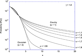
Figure 21. Levy stable probability distribution functions from α = 1 (Cauchy) to α = 2 (Gaussian) plotted against the Lévy-function argument.
Download figure:
Standard image High-resolution imageIn anomalous transport, either or both distributions Ψ(τ) and ρ(τ) for persistence times and rest times can have Lévy stable distributions. To distinguish between these possibilities, the Lévy exponents will be represented by α and β, respectively. The participation of the exponents α and β in the subdiffusive or superdiffusive character of the transport depends on the range of the exponents and on their combination. The possible combinations in the long-time limit are shown in table 3 [294]. If the resting time is exponentially distributed (regular) and 1 < α < 2 then superdiffusion results. However, for smaller values of the power 0 < α < 1 the transport becomes ballistic in the sense that the mean persistence length, even for finite sampling, can exceed the size of the observation volume. Conversely, if the transport length is exponentially distributed (regular) and the resting-time exponent has the range 1 < β < 2 then the net transport remains diffusive, only becoming subdiffusive for much smaller powers 0 < β < 1. There is also the possibility of mixed behavior when there is a competition between divergent persistence lengths and divergent resting times.
Table 3. Long-time limits of the CTRW model [301].
| Length: regular | Length: 1 < α < 2 | Length: 0 < α < 1 | |
|---|---|---|---|
| Rest time: regular | Brownian diffusion | Superdiffusion | Ballistic (Levy flight) |
| Rest time: 1 < β < 2 | Brownian diffusion | Superdiffusion | Ballistic (Levy flight) |
| Rest time: 0 < β < 1 | Subdiffusion | Mixed or subdiffusion | Mixed |
Within the cellular environment, transport cannot have strictly divergent moments because of the finite size of the cell and the finite size of intracellular components. In cell biology, the heavy tails of Levy distributions within the cell are truncated and the probability density vanishes above a set size. This is known as a truncated Lévy distribution. Because of this finite cutoff, all moments of a truncated Levy distribution are convergent, and in the long-time limit all processes converge on Gaussian processes. A rough rule of thumb for the maximum range is half the diameter of a cell. Typical epithelial cells have diameters around 10 μm, setting the limited range of motions to approximately Lmax = 5 μm. For intracellular transport, this sets a maximum Doppler number at NDmax = qLmax = 60 although many processes will be limited to about a micron, such as membrane undulations or transport inside the nucleus, limiting the maximum Doppler number for these processes to approximately NDmax = 10. Despite this transformation from anomalous to regular statistics with truncation, the convergence is slow and is slower for heavier tails. In the intermediate-time limit, experiments that measure transport only within finite ranges often observe anomalous exponents. However, in the short time limit, all actively-driven processes, whether truncated or not, are ballistic.
4.5.2. Levy persistence-time distribution.
To gain some intuition about light scattering from Lévy walks, Monte Carlo simulations provide an easy path to visualize distributions of transporting particles as well as the central probability distribution W(x,t). A Monte Carlo simulation of the one-dimensional trajectories of 50 Levy walkers with a uniform speed with α = 1 (Cauchy distribution) and with no resting time is shown in figure 22(a). Many walkers have persistent flights within the time frame that produce a superdiffusive spread of positions. The distribution function W(x,t) is shown in figure 22(b). At very short times, it is composed of a delta function traveling at the ballistic speed of the walkers. At later times, the decreasing-amplitude delta-function on the leading edge represents the surviving fraction of ballistic walkers, while the positions of 'scattered' walkers develop into a diffusive distribution as the delta function vanishes.
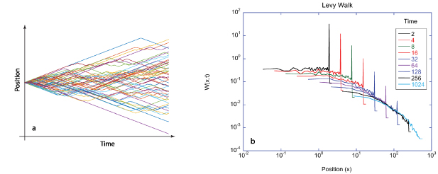
Figure 22. Stochastic simulations of displacements for v = 1 μm s−1, α = 1, γ = 1, and tp = 0.5 s. (a) Position vs. time for 50 one-dimensional Levy walkers (no rests) that all start at the origin with the same speed. The persistence lengths are Levy distributed. (b) The probability distribution function (PDF) for a group of walkers with a Cauchy distribution of persistence lengths for successive times.
Download figure:
Standard image High-resolution imageThe RMS displacements for 1D walks are shown in figures 23(a) and (c). The Levy walk remains ballistic (superdiffusive) throughout the time range. The associated homodyne and heterodyne spectra from the simulations are compared in figures 23(b) and (d) to regular transport (Laplacian distributions). The Doppler number for the regular transport is ND = 3. The persistent motion of the walkers for the Cauchy distribution produces an effective Doppler number ND > 3 with an enhanced Doppler peak in the spectra. The isotropically averaged case is shown in figures 23(b) and (d) showing the Doppler peak converted to a Doppler edge in the spectra. The power-law slope of the spectral density above the edge is steeper than −2, which is a signature of the Doppler effect from the transport. Experimental studies of light scattering that display steep slopes above the edge are one direct indication of persistent transport in the sample.
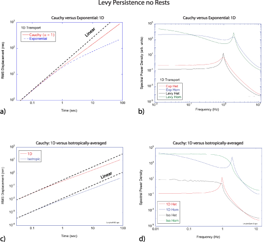
Figure 23. Stochastic simulations of Levy walks for Cauchy (α = 1) distribution of persistence lengths with no rests for 1D transport with v = 300 nm s−1 and tp = 0.5 s. (a) Mean-squared displacement for regular (decaying exponential) and Levy transport as a function of time. The Levy transport remains superdiffusive through late times. (b) Power spectra (homodyne and heterodyne) for one-dimensional walkers with regular compared with Levy persistence length distributions as a function of frequency. (c) Mean-squared displacements for one-dimensional and isotropically averaged Levy walks. (d) Comparison of power spectra of one-dimensional and isotropically averaged Levy walks.
Download figure:
Standard image High-resolution imageUniform velocities are not observed in living systems which are governed by probability distributions. For instance, the maximum speed for organelle transport by a single motor protein sets an upper bound for the speed, but variable local environments reduce individual organelle speeds to a range of lower values. Figure 24 shows 1D transport for a Levy persistence length and no resting for three speed distributions: uniform speed (a delta function speed distribution at 300 nm s−1), a uniform distribution between zero and the maximum speed of 300 nm s−1, and an isotropic average of the uniform speed distribution. The uniform speed distribution produces the same spectrum as the 1D isotropically averaged case in figure 23(d), because the average speeds for isotropic averaging is formally equivalent to uniformly distributed speeds. The maximum speed still produces a sharp Doppler edge. When the uniform speed is isotropically averaged, the heterodyne spectrum retains a Doppler edge, but in the homodyne spectrum the Doppler edge is significantly softened. This is the general trend for Doppler light scattering in living tissue. Although individual persistence lengths may yield Doppler numbers well into the Doppler regime, broad speed distributions and isotropic averages convert Doppler edges to spectral shapes that may be difficult to distinguish from diffusive spectra.
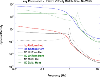
Figure 24. Stochastic simulations of Levy distribution of persistence lengths (no rests) for 1D transport, 1D uniform speed distribution, and isotropically-averaged uniform speed distribution for heterodyne and homodyne detection with v = 300 nm s−1, α = 1, tp = 0.5 s. The uniform distribution of speeds in 1D give the same results as the isotropically-averaged constant-speed case of figure 23(d), but isotropic averaging of the uniform distribution further softens the Doppler edge.
Download figure:
Standard image High-resolution image4.5.3. Levy resting-time distribution: subdiffusion limit.
In the long-time limit, a simple analytical model of subdiffusion is obtained from the CTRW model with exponentially distributed (regular) persistence lengths and Levy-distributed (anomalous) resting times. The PDF in the long-time limit is [302]
for 0 < β < 1. The MSD for Levy resting times is
where β = 1 is the Brownian diffusion limit. As β decreases from unity the transport becomes more subdiffusive. The probability distribution function is shown in figure 25 for β = 0.5 (subdiffusive) compared to β = 1 (Brownian). The Levy waiting-time distribution creates sharper features and narrower distributions.
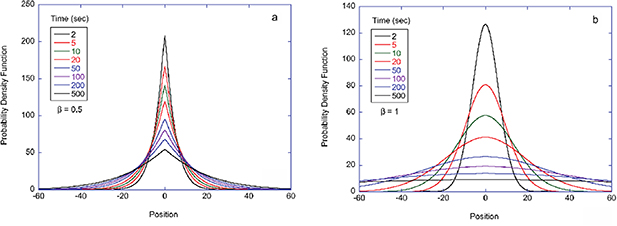
Figure 25. Probability distribution function W(x,t) for the Levy resting-time model for (a) β = 0.5 and (b) the Brownian distribution β = 1.
Download figure:
Standard image High-resolution imageThe modes for different wavenumbers q in the distribution function W(q,t) decay as Mittag–Leffler functions that replace the simple exponential decay of Brownian diffusion with the decay function

where the Mittag–Leffler function is
The time dependences of the decay of W(q,t) for a given q and a range of values for β are shown in figure 26(a). The temporal Fourier transforms W(q,ω) are shown in figure 26(b). The Cauchy distribution of resting times for β = 1, though having a divergent mean, produces a conventional diffusion spectrum. As the exponent decreases below unity, the Doppler edge converts to a 1/f spectrum.
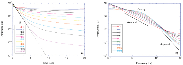
Figure 26. (a) Mittag–Leffler functions versus time extending from the exponential (β = 1 dashed) to the extreme tail regime. (b) Fourier transforms of Mittag–Leffler functions versus frequency from the Cauchy limit to the subdiffusive regime.
Download figure:
Standard image High-resolution imageThe asymptotic short-time behavior of W(q,t) is
and the asymptotic long-time behavior is
The long-time behavior is also expressed as an infinite series
Monte Carlo simulations of fluctuation spectra for one-dimensional transport with Laplacian persistence distribution and Lévy resting times are shown in figure 27 for ND = 3 compared to exponential resting times. The subdiffusive character of the heavy-tail resting times produces an rms displacement that scales with time with a reduced exponent. It also reduces the effective Doppler number and produces a diffuse knee. A new feature appears in the homodyne spectrum in the case of Levy resting times. The Doppler peak in the homodyne spectrum occurs at the Doppler frequency rather than at twice the Doppler frequency, which was the usual situation for all previous cases studied above. This effect is caused by 'self heterodyning'. The divergent resting times produce a substantial population of stationary scatterers that scatter light with no Doppler shift, acting as 'internal' local oscillators. These local-oscillator partial waves beat against the Doppler-shifted frequency of the moving population, producing a pseudo-heterodyne spectrum even in the case of no external reference wave.
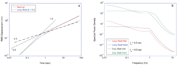
Figure 27. Stochastic simulations of displacements and power spectra for 1D (not isotropically averaged) Laplacian persistence lengths with Lévy resting times and uniform speed of 300 nm s−1. The characteristic values are tp = 0.5 s and tw = 0.5 s with α = 1 and β = 0.5. (a) RMS displacement versus lag time. (b) Power spectra versus frequency. The double peaks in the homodyne spectra are the result of self-heterodyne of moving walkers against stationary ones.
Download figure:
Standard image High-resolution image4.5.4. Levy persistence and resting-time distributions: mixed case.
When both the persistence lengths and the resting times have Lévy stable distributions, a mixture of behavior results. An example is shown in figure 28 that compares normal transport having ND = 3 to the mixed case with α = 1 and β = 1 (Cauchy) and tp = 0.5 s and tw = 0.5 s. In the normal transport case, the RMS displacement starts ballistically and transitions to diffusive at long times. The mixed Lévy case starts with super-ballistic displacements and transitions to ballistic at long times. The corresponding fluctuation power spectra in figure 28(b)) show the clear Doppler peak (for one-dimensional transport) caused by the Lévy tail on the persistence length despite the heavy tail on resting times. The self-heterodyne peak in the homodyne spectrum is much more distinct in this case.

Figure 28. Stochastic simulations for one-dimensional motion with v = 300 nm s−1 and ND = 3 for regular (exponential tp = 0.5 s) and Levy persistence and waiting times (tp = 0.5 s and tw = 0.5 s with α = 1 and β = 1). (a) RMS displacements versus lag time. (b) Power spectra versus frequency for 1D (not isotropically averaged) mixed Lévy transport (Levy persistence and rests) compared to normal transport (decaying exponential persistence and rests). Compare (b) to figures 21(b) and 25(b).
Download figure:
Standard image High-resolution image4.5.5. Fractional Brownian motion (fBm).
Fractional Brownian motion (fBm) is an alternative approach to anomalous transport that connects with Levy statistics in some limits [303]. The trajectories generated by fBm statistics have self-similar structures related to Hurst exponents [304] and arise in many transport systems such as finance and turbulence [292, 294, 305]. In the context of biological transport, fBm can yield a continuous range of behavior from subdiffusion, through conventional diffusion, to superdiffusion without the divergent moments associated with the heavy tails of the Levy distributions. Fractional Brownian walks are non-Markovian, and superdiffusion is caused by correlations among successive steps rather than by large excursions in single steps. Subdiffusion is caused by anticorrelations among successive steps.
Simulations of fractional Brownian statistics can be implemented through Monte Carlo simulations using Cholesky decomposition. A discrete matrix is constructed through
for integers t, s = 0:N + 1 to describe a walk of N steps where H is the Hurst exponent. This matrix is decomposed into the square root matrix Σ such that Σ2 = Γ through Cholesky spectral decomposition. If the eigenvalues and eigenvectors of Γ are λi
and  , then the matrix Σ is given by
To generate a walk of N steps, construct a sampling of N + 1 values  from the normal distribution, then construct the fractional random walk by the matrix product

The N individual steps of the walk are the differences  . For H = 0.5 this yields the conventional random walk. For 0 < H < 0.5 this produces subdiffusion, and for 0.5 < H < 1 this produces superdiffusion. Examples of fractional Brownian walks are shown in figure 29 for H = 0.15, H = 0.5 and H = 0.85. The persistence and correlated motions for the high Hurst exponent produce smoother trajectories with larger MSDs than for normal diffusion. The anticorrelations for the Hurst exponent less than 0.5 produce rapidly fluctuating trajectories with smaller MSDs. The MSD and the power spectra for 1D motion are shown in figure 30 for H = 0.15, 0.5 and 0.85.
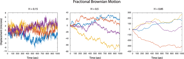
Figure 29. Fractional Brownian walks for H = 0.15, 0.5 and 0.85 plotting displacement versus time. The conventional random walk occurs for H = 0.5, and subdiffusion and superdiffusion occur for H = 0.15 and H = 0.85, respectively.
Download figure:
Standard image High-resolution image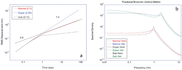
Figure 30. Fractional Brownian motion with superdiffusive and subdiffusive behavior for H = 0.85 and H = 0.15, respectively. The speed is v = 300 nm s−1 with tp = 0.5 s. (a) RMS displacement versus lag time. (b) Power spectrum versus frequency.
Download figure:
Standard image High-resolution image4.5.6. Aging in anomalous transport.
Aging in transport is a form of non-stationary behavior for which particles that initially diffuse (or walk) freely are ultimately constrained by their environment [133]. For instance, this is a well-established model for molecular diffusion within cell membranes [306] in which the membrane is composed of compartments which corral molecules within so-called picket fences. Organelle transport also clearly has this limited transport when the organelle displacement exceeds the persistence length of cytoskeletal elements, and cell membrane motions are limited when they approach the scale of the cell. These simple size-limit constraints enter anomalous transport as an aging process in which the effective diffusion coefficient is time dependent (the coefficient 'ages') and vanishes for times longer than the diffusion time to reach the compartment limits. This kind of aging causes subdiffusive behavior. It is also possible to have diffusion coefficients that increase with time, for instance through directed transport, leading to superdiffusive behavior.
A model that captures these behaviors is scaled Brownian motion with a time-dependent diffusion coefficient given by

leading to transport that is subdiffusive for 0 < η < 1 and superdiffusive for η > 1, with normal diffusion for η = 1. This form of aging has been incorporated into CTRW simulations and compared with analytical results in [307]. Several non-intuitive trends emerge from analysis of the MSD under conditions of aging, such as a shorter ballistic regime under superdiffusion and a longer ballistic regime under subdiffusion.
The MSD for an aging process is calculated after an aging time ta, for which the MSD is [307]
which integrates the two-time velocity correlation function. In the CTRW model, when the aging time is the longest time scale in the problem, the long-time behavior is normal diffusion independent of η. However, when the observation time exceeds the aging time, then anomalous transport is observed with characteristic power law dependence on η.
A comparison of normal transport to aged transport with η = 0.5 is given in figure 31 showing the spectral density and MSD. The aging causes decreasing displacements with increasing time, leading to a spread of Doppler frequencies and a loss of the Doppler peak (for one-dimensional non-angle-averaged motion). The MSD is ballistic at short times in both cases but becomes sub-diffusive at long times for the aged case. Aging in the transport properties produces spectra that are broadened and have no distinct Doppler edge. The Wiener–Khinchine theorem breaks down for aging transport so that the power spectrum is no longer the same as the Fourier transform of the autocorrelation function. However, even in this case for η = 0.5, the Wiener–Khinchine theorem still holds approximately because the diffusion coefficient is changing slowly relative to the sampling rate.
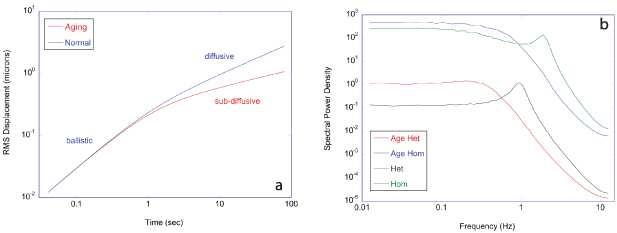
Figure 31. Effect of aging on one-dimensional CTRW simulations comparing normal to aged transport processes with v = 300 nm s−1, tp = 0.5 s and for an aging parameter η = 0.5. (a) MSD versus lag time for normal and aged transport. (b) Spectral density for normal and aged transport. Both are ballistic at early times, but the decreasing diffusion coefficient for the aged process produces sub-diffusive behavior.
Download figure:
Standard image High-resolution image4.5.7. Summary of anomalous transport.
Transport within the intracellular environment is extremely complex, with active processes that tend to produce superdiffusive motion balanced by a crowded cytosol and by intermittent processes that tend to produce subdiffusive motion. Anomalous transport is prevalent on both sides of this balance for all intracellular super-molecular structures. Smaller molecules may experience thermal diffusion within the cytosol, as observed using FCS [192, 194], but even these processes can have anomalous transport [197].
The CTRW model is a particularly relevant computational tool for exploring the effects of different types of anomalous transport on the Doppler light scattering spectra that might be detected in an experiment. CTRW easily incorporates persistent motion punctuated by durations of rest, and it easily incorporates Levy stable persistence and resting times. The Levy stable distributions are more general and powerful for exploring intracellular transport than normal probability distributions. As the characteristic exponents of the Levy processes change, it is possible to recover regular transport for some ranges of exponent values, while for other ranges of values, anomalous transport emerges naturally, either superdiffusive or subdiffusive. Of particular interest is a balance between divergent persistence times and divergent resting times, where the superdiffusive effects are compensated by the subdiffusive effects. In addition, the coexistence of divergent persistence and rests produces interesting changes in the Doppler fluctuation spectra, in particular the possibility of 'self-heterodyning' of light scattered from moving objects against light scattered from momentarily stationary objects. The self-heterodyne situation under homodyne scattering conditions (without an external reference wave) creates homodyne Doppler peaks or edges at the characteristic Doppler frequency rather than at twice the frequency. Such signatures, if they could be detected using local light-scattering probes, would lend insight into the competition between superdiffusion and subdiffusion in intracellular transport.
Despite the competition between superdiffusion and subdiffusion, and the prevalence of directed active motion within the cytosol (that might seem to favor superdiffusive behavior), intracellular transport falls intrinsically in the sub-diffusion regime for long-time correlations. This is because the length scales involved with all intracellular transport are limited by the size of the cell or by the size of compartments within the cell, and all intracellular motion is spatially limited. This is particularly important for processes that may have Levy behavior for short runs, but all spatial Levy distributions must be truncated. This immediately allows moments of the distribution of persistence lengths to converge to finite values. The absence of heavy-tail outliers reduces otherwise superdiffusive signatures back to normal signatures. On the other hand, heavy tails in the rest-time distribution are not limited by spatial sizes and may still diverge, inducing subdiffusive signatures. Therefore, superdiffusion at long correlation times is not a characteristic of living tissue, although either subdiffusion or superdiffusion or a mixture may be observed at short time scales.
5. Detection of cellular motion and intracellular transport using coherent light scattering
DLS dates back to the work of Smolokowski and Einstein on light scattering from thermal fluctuations of liquids [308, 309]. The advent of the laser opened the field to coherent light scattering studies through the Doppler effect [310, 311]. Many of the early studies using DLS were on dilute systems such as colloidal solutions [312, 313] and motile bacterial populations in liquids [314, 315] where the small Doppler shifts were detected using optical mixing. The shape of the Doppler spectrum could be used to extract important physical properties of the dynamic motions within these systems such as diffusion constants and drift speeds [117].
DLS from living tissue shares similarities with the fluctuation spectra observed from diffusion in colloidal solutions. These similarities are superficial, because (as discussed in section 3) transport in living tissue is highly active, far from equilibrium, and is not diffusive, being composed of random sets of persistent piece-wise constant drifts. DLS then becomes an important tool for extracting the active transport processes of living cells and tissues. Conventional techniques in this area include quasi-elastic light scattering (QELS), diffuse-correlation spectroscopy (DCS), DWS, and the coherence-gated techniques of dynamic-contrast OCT, tissue-dynamics spectroscopy (TDS) and differential dynamic microscopy (DDM). Direct imaging of intracellular dynamics inside living tissue is also becoming possible with the advent of super-resolution microscopy [108], but this does not rely on coherent light scattering and will not be part of this review.
5.1. Quasi-elastic light scattering (QELS)
QELS relates to the scattering of light by temporal fluctuations of spatial refractive index inhomogeneities. The term quasi-elastic specifically describes the small frequencies associated with modulations of the incident light frequency. Center frequencies in the visible are around 1014 Hz, while the frequencies associated with index fluctuations are typically in the range from sub-Hz to hundreds of Hz. The term quasi-elastic also implies single-scattering or minimal multiple scattering that may include multiple small-angle forward scattering plus a single large-angle scattering event. The term generally excludes high-multiplicity multiple scattering that is more generally treated by DWS and diffuse correlation spectroscopy, discussed in later sections.
As described extensively in earlier sections of this review, there are two limiting behaviors for DLS: the diffusive limit and the Doppler limit. When transport lengths are much shorter than the reduced wavelength, for instance in the case of thermal Brownian motion of macromolecules, then there is no Doppler effect and the fluctuations are purely diffusive. In the other limit, when the transport lengths are much longer than the reduced wavelength, even if the average motion of an ensemble is isotropic, then the light scattering is in the Doppler limit, and the fluctuation frequencies are directly related to the mean speeds involved in the transport. In living tissue, transport is mainly isotropic when averaged over sufficiently many cells, and the Doppler behavior is observed in the side-band spectrum even when the average Doppler frequency vanishes.
The earliest work on QELS began shortly after the invention of the laser in 1960. Dynamic laser speckle was recognized early as a consequence of the internal dynamics of light-scattering systems [312, 313, 316–318]. Interest expanded from studies of macromolecules and small particles to include the motions of larger-scale systems such as membranes and gels [319–321] and systems in thermal non-equilibrium [322]. These studies soon included light scattering from living cells, especially erythrocytes [256, 323] and active bacteria motions [324, 325], and intracellular dynamics [326, 327] that resolved speeds down to 100 nm s−1. The general field of dynamic speckle fluctuations expanded rapidly to become a major analytical tool in biology and chemistry [118, 328–330]. Recent directions of QELS research includes biomedical studies of tissue and cartilage [331] and opthamology [332].
5.2. Dynamic-contrast optical coherence tomography (OCT)
Long-coherence light scattered from translucent volumetric heterogeneous targets, such as medical biopsies, produces partial waves from all depths, generating speckle that has little or no depth discrimination. To localize the regions in a scattering volume from which dynamic speckle is generated it is necessary to introduce depth discrimination into the speckle detection mechanism. This can be accomplished through OCT [106, 333–337]. There are three distinct classes of OCT: (1) coherence-domain; (2) Fourier-domain; and (3) image-domain. These use different detection mechanisms.
Coherence-domain OCT was the original class of OCT that was developed by Fujimoto et al at MIT [333, 338–343]. It uses coherence-domain laser ranging [344] with low-coherence laser sources for which partial waves interfere only when they share the same optical path length. In a heterodyne situation with a low-coherence reference matched to the object wave, the light can be localized to an effective optical section inside a tissue target by matching the optical path length of the scattered waves to the reference waves. Scattering from successive depths is acquired by scanning a delay line in the reference arm of an interferometer to generate what is called an A-scan. Translating an A-scan in a transverse spatial direction across a sample generates a B-scan. The reliance on dual scanning (depth and one transverse dimension) makes this form of OCT slow to collect volumetric information.
An alternative to mechanical scanning in depth is through the use of spectral interferometry [345] which is the basis of Fourier-domain OCT [346–348]. Spectral interferometry encodes depth information in spectrally dispersed interferograms, allowing A-scan depths to be reconstructed through a Fourier transform of interference fringes in a spectrogram, and no scanning is required in the case of a fixed spectrum light source. Alternatively, a swept-frequency narrow-band light source can be used to generate the spectral interferograms. The sweep frequencies of these sources can be high, in the range of 100 000 A-scans per second, making the depth scanning much faster than for coherence-domain OCT, but transverse mechanical scanning is still required to generate volumetric representations of the target sample.
Instead of scanning in depth as the fundamental signal acquisition, image-domain OCT (also known as en face OCT or full-frame OCT) [349–356] selects a fixed depth inside the scattering volume by setting a delay on a reference wave using a low-coherence light source and generates an instantaneous two-dimensional image for two transverse spatial dimensions. The coherence gate to capture the image can be through holography [349] or direct imaging in a microscope [351]. The simultaneous illumination of multiple spatial channels in image-domain OCT creates a higher speckle background through what is called channel crosstalk. This can be suppressed by using broader-band light sources, or can be utilized to enhance speckle, for instance for DLS and FS. At a fixed depth, image-domain OCT is the fastest form of OCT for generating time-resolved speckle patterns.
In coherence-domain and image-domain OCT, the detection uses a low-coherence continuous source, such as a superluminescent diode, for which light sharing the same optical path length as the reference produces interference fringes. The spatial path-bandwidth product of a continuous-wave source with a Gaussian spectrum is  . In a backscatter geometry the momentum change is q = 2k, giving
as the depth resolution for coherence-gated backscatter imaging. This longitudinal resolution is half of the coherence length of the light source because of the backscatter configuration. As an example, a light source centered on 840 nm with a bandwidth of 50 nm has a lower bound on longitudinal resolution of 6 μm.
Multiple scattering and optical aberrations of light propagating through tissue broadens the resolution as a function of the depth inside the tissue at which the coherence gate is set. For instance, in the above example, at a coherence depth set at d = 500 μm inside a tissue sample, the longitudinal resolution, in the absence of confocal spatial filtering, is broadened to roughly  = 50 μm, where g is the anisotropy factor of tissue. This is the typical longitudinal resolution of full-field optical-coherence imaging (OCI) at nominal half-millimeter depths. On the other hand, conventional OCT is typically performed with high-NA optics which introduces a confocal spatial filter that restricts the broadening to values closer to the theoretical limit. Adaptive optics also can be used to remove the optical aberrations to retain values closer to the ideal limit set by the coherence of the source [357].
The ubiquitous phenomenon caused by coherent light scattering from living tissue is a speckle field that changes in time, i.e., dynamic speckle. As discussed extensively in the earlier sections of this review, the dynamics are caused by multiple light scattering from intracellular motions from the cells inside the living tissue. Because there is a wide range of intracellular components as well as sizes and speeds, the speckle can be highly active with significant temporal fluctuations that can be used to generate speckle contrast for imaging. When combined with low-coherence interferometry to gate light scattered from selected depths, coherence-gated speckle contrast imaging was the first form of dynamic OCT developed to interrogate multicellular tumor spheroids [358] and tissue culture [359].
The first three-dimensional en face OCT imaging of living-tissue speckle contrast imaging was performed on multicellular tumor spheroids grown to a large size of about 1 mm diameter in a bioreactor [360]. The speckle contrast images are shown in figure 32 at successive coherence-gated depths. The images are color coded for speckle temporal contrast through normalized standard deviation. The outer shell of the tumor spheroid consists of proliferating cells that are metabolically highly active, producing high temporal contrast (reds and oranges). Deeper inside the spheroid, the nutrients and oxygen are depleted beyond approximately 200 μm from the spheroid surface, leading to a hypoxic core with reduced metabolic activity (greens and blues). Because the tumor spheroid growth in the bioreactor takes weeks, the extended hypoxic conditions in the core also produce necrotic regions that are essentially static. However, multiple forward scattering from the overlying layers produces a 'shimmering showerglass' effect that superposes a weak temporal speckle contrast on the necrotic core. The dynamic range in speckle dynamic contrast between the proliferating shell and inactive core indicates that the shimmering shower-glass is no larger than about 40% and may be smaller because of residual activity inside the core.

Figure 32. Dynamic OCT speckle contrast images of a living 800 μm diameter tumor spheroid at depths (from top left to bottom right) 60, 120, 190, 250, 330, 390, 460, 530, and 600 μm. The scale bar is 100 μm and the color scale is from 40% to 100% speckle contrast. The cellular motility (normalized standard deviation) at selected depths shows the proliferating shell surround the hypoxic and necrotic core. [Reprinted/Adapted] with permission from Jeong et al [360] © The Optical Society.
Download figure:
Standard image High-resolution imageThe interferometric detection principle behind OCT enables the reconstruction of complex scattered amplitudes in field-based OCT to study DLS to track diffusive particle dynamics [361], to distinguish directional from diffusional transport [362–365], and to differentiate stromal and epithelial layers [366]. There is significant interest in flow in the medical context of tissue perfusion, and DLS OCT provides a transport tool [365, 367] that is complementary to Doppler-based OCT [368–370]. Dynamic OCT initially expanded into studies of apoptosis [105, 371, 372], chemosensitivity of tissues to chemotherapies [360, 373, 374], viability of oocytes and embryos [375], and to improve image contrast in OCT [376]. Applications of dynamic OCT include subcellular metabolic activity [105, 377–380], extracellular matrix remodeling [381], and drug response of tissues [360, 374, 382–384]. It has also been applied to studies of plasma flow [385, 386], dermatology [387], eye drainage [388], and embryology [389–391]. For potential use for drug development and diagnostics, dynamic OCT has been used to characterize three-dimensional tissue culture [383, 392, 393], and for testing chemotherapy cancer drug efficacy in animal preclinical trials [394, 395] and in human clinical trials [396, 397]. Some of these applications are highlighted in figure 33.
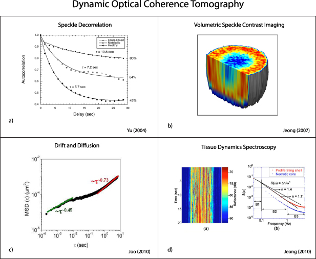
Figure 33. The early development of dynamic optical coherence tomography for intracellular dynamics. (a) Coherence-gated speckle decorrelation times for healthy and poisoned tissue culture. Reproduced from Yu et al [358]. CC BY 4.0. (b) Dynamic OCT of speckle contrast inside large tumor spheroid showing the hypoxic core surrounded by the proliferating shell. Reproduced from Jeong et al [360]. CC BY 4.0. (c) Mean-squared displacement versus time in OCT speckle images of diffusion and flow. Reproduced from Joo et al [362]. CC BY 4.0. (d) Tissue dynamics spectroscopy performed using dynamic OCT. Jeong et al [399]. CC BY 4.0.
Download figure:
Standard image High-resolution image5.3. Tissue dynamics spectroscopy (TDS)
The central analysis tool used in dynamic OCT is FS to obtain the frequency-dependent spectral power density of tissue dynamics. TDS combines the FS of DLS [118, 398] with OCT to extract changes in the Doppler spectra of intracellular dynamics, for instance when living tissue is challenged by environmental or exogenous agents [105, 399]. The Doppler spectra of active transport in living tissue is broadband, ranging from 10 mHz (or lower) up to tens of Hz. The transport is generally isotropic and contains contributions from a wide range of processes with widely different characteristic speeds. These factors yield Doppler spectra that are broadband and have only a few quantifiable features. These features include: (1) an edge (or knee) frequency associated with the average speed of intracellular transport, (2) a slope parameter that characterizes the rate of decrease of spectral power with increasing frequency above the knee frequency, (3) a Nyquist floor near the Nyquist sampling frequency, and (4) a low-frequency plateau. These features are illustrated in figure 34.

Figure 34. Intracellular Doppler spectrum of a healthy A2730 multicellular tumor spheroid on a log–log scale. The primary features of the spectrum are the low-frequency plateau, the knee frequency, the slope, and the Nyquist floor. The dynamic range depends on the other feature values. This typical spectrum spans three orders of magnitude in frequency and almost three orders of magnitude in vertical dynamic range. The log–log slope is typically between −1.5 and −1.7 for many tissue types. These data were acquired at 25 fps for 80 s with an exposure time per frame of 10 ms.
Download figure:
Standard image High-resolution imageA differential approach is used in which a baseline spectrum is established to which spectral density changes are referenced after the application of a perturbation. The relative change in spectral density is captured through the log difference of the spectrum at times after the perturbation is applied relative to the baseline before the perturbation through

where t0 is the baseline time and ν is the frequency. The time-frequency representation of the log difference is the drug-response spectrogram. An example is shown in figure 35 for the reference drug colchicine applied to a DLD-1 tumor spheroid. The baseline spectrum and the final spectrum are shown in figure 35(a) and the time-frequency spectrogram is shown in figure 35(b) for data acquired during 9 h after the application of the drug. Colchicine inhibits tubulin polymerization, degrading the microtubule cytoskeleton. The action of colchicine on the DLD tissue dynamics induces increased spectral density at the Nyquist floor associated with increased organelle activity, increased spectral density at the low frequencies associated with membrane and cell shape changes, and inhibition in spectral content in the mid frequencies associated with the knee and power-law slope.

Figure 35. Spectra and spectrogram for colchicine applied to a DLD tumor spheroid at 25 fps for 80 s and 10 ms exposure. (a) The baseline spectrum and the final spectrum as functions of frequency after application of 25 μM Colchicine. (b) The differential drug-response spectrogram displaying the change in spectral content as a function of time (vertical axis) and average intracellular speed (horizontal axis) where the Doppler frequency shift is converted to intracellular speed for the backscatter configuration at a wavelength of 840 nm. The drug is applied at t = 0, and the spectral changes are relative to the baseline spectrum prior to the application of the drug.
Download figure:
Standard image High-resolution imageThe differential format of TDS captures subtle changes in intracellular motion caused by exogenous agents or environmental changes, and TDS presents a form of phenotypic profiling for potential drug screening applications [400] that seek to identify physiological responses of tissue to drug leads early in the drug-development pipeline. For instance, a study of several different reference drugs found significant differences among classes of drugs with different mechanisms of action (MoA) [401]. A subsequent study of Raf inhibitors on two different tissue types that contain wild-type versus mutated BRAF receptors found differing efficacies for these potential anti-cancer drugs in the two tissue types [374]. High-throughput drug screening relies on three-dimensional tissue culture that can be grown in different formats, such as hanging-drop [402], U-bottom plate and bioreactor growth approaches. Tissue dynamic screens of common drugs on tissues grown using the different formats show different spectral responses to the same drug [392], highlighting the importance of the context of the three-dimensional environment for potential drug screening applications that may depend on the role played by cellular adhesions [403]. Biodynamic imaging and TDS have also been used to monitor the metabolic activity of oocytes and embryos for potential IVF applications [375, 390, 391].
Typical sample sizes for TDS range from 100 μm diameter to 1 mm diameter. For the larger sample sizes, the fluctuation spectra can be averaged over the entire sample to yield high signal-to-noise performance. However, it is well known that cancer tissue is highly heterogeneous with pronounced spatial and genetic variability. Therefore, tissue dynamics spectroscopic imaging (TDSI) creates tissue-scale spatial maps of the different changes in spectral content over a sample optical section. The drug-response spectrograms can be converted to features by time-frequency filters to isolate specific spectral changes such as red- or blue-shifts or second-order effects. The output values from these filters represent quantitative spectral features that can be measured across a sample. An example is shown in figure 36 that tracks red- and blue-shifts along one color axis and broadband inhibition/excitation across another color band in a four-color merge. The resulting sample TDSI map of the drug response is shown in figure 36(b) compared to optical maps and histology in figures 36(c) and (d), respectively [404]. Further examples of the four-color merged TDSI maps are shown in figure 37 for esophageal cancer pinch biopsies, displaying the wide range of spectral shifts that occur within relatively small samples of only about 1 mm3. This heterogeneity can provide insights into the complexity of the cancer for individual patients and may help guide personalized medical interventions.
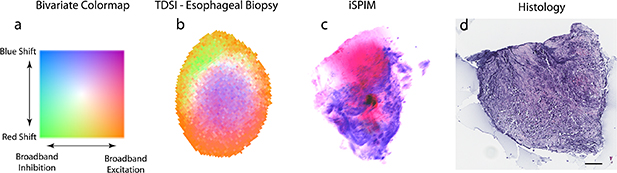
Figure 36. Tissue dynamics spectroscopic imaging (TDSI) of a human esophageal pinch biopsy sample [404]. (a) Bivariate colormap representing broadband inhibition and blue shift. (b) Bivariate TDSI map of human esophageal biopsy responding to 5-fluorouracil (5-fu). (c) An iSPIM image with DRAQ 5 (blue) and Eosin (pink) for the same sample in (a), and (d) histology image. Reproduced from Li et al [404]. CC BY 4.0.
Download figure:
Standard image High-resolution image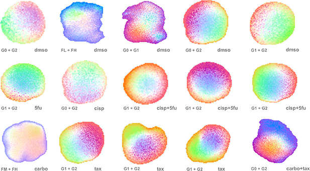
Figure 37. Examples of merged four-color TDS images of human esophageal biopsies showing sample-to-sample variability in drug responses. The color scheme uses contrasting colors for positive and negative values of the spectral signatures. The spectral signatures FL, FM, and FH represent low, mid and high frequency, respectively, and G0, G1 and G2 represent broadband response, red/blue shift, and central-frequency shifts, respectively. Lower right corners designate drug treatments. Drug abbreviations: DMSO, 0.1% DMSO in growth medium (used as a negative control); cisp, 25 μM cisplatin; 5fu: 25 μM fluorouracil; tax, 5 μM paclitaxel; carbo, 25 μM carboplatin. '+' indicates a combination of two drugs. Reproduced from Li et al [404]. CC BY 4.0.
Download figure:
Standard image High-resolution imagePhase-sensitive TDS is an extension of TDS that uses complex amplitudes reconstructed by digital holography [405]. In addition to direct Doppler peaks that can be resolved spectroscopically for directed motion, it makes it possible to construct phase PDFs. One example is shown in figure 38 for a healthy DLD-1 tumor spheroid. The PDF is relatively flat up to phase fluctuations of 0.1 rad, after which the probability falls off in a power law. The sampling rate for these data is 25 frames per second. To avoid the phase-wrapping problem, the phase displacements are acquired between consecutive reconstructed holograms. Gaussian and Cauchy distributions are shown for comparison to the best fit to the data by a Levy stable distribution with α = 1.6. The Gaussian (α = 2) and the Cauchy (α = 1) distributions are limiting cases of Levy distributions that are characterized by 'heavy tails' of probability. Levy phase distributions from light scattering may arise from Levy flights by subcellular components of the living tissue [297].
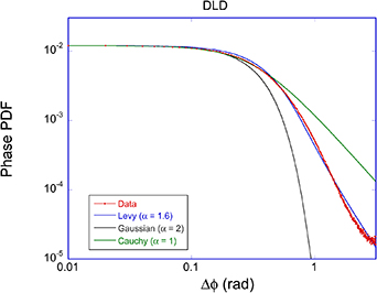
Figure 38. Phase probability distribution function (PDF) for phase-sensitive detection of intracellular motion in DLD-1 tumor spheroids. The best fit to the data is a Levy stable distribution with α = 1.6.
Download figure:
Standard image High-resolution imageRelated phase-sensitive techniques that are used for optically-thin quasi-2D samples include quantitative phase imaging (QPI) [152, 156] and quantitative phase digital holography [153, 154, 406, 407]. These techniques perform phase unwrapping [408–410] to recover the optical thickness of cell and tissue samples. This approach can be used in live-cell imaging to track dynamic changes in two-dimensional cells and tissue culture [411–414]. However, quantitative phase techniques generally break down in optically thick tissue samples that have multiple scattering, although recent approaches have been proposed to extend QPI into thicker samples [415–417].
An emerging application for biodynamic imaging and TDS is chemoresistance testing on cancer biopsy samples to predict whether patients will respond to their chemotherapy. A preclinical trial of 19 dogs with B-cell lymphoma was performed to test the in vitro response of the lymphoma biopsies to CHOP therapy that is a combination of doxorubicin, prednisolone, vincristine and cyclophosphamide [395]. The same therapy is used to treat human B-cell lymphoma. The dogs either responded well to the treatment and had a progression-free survival time greater than 100 d (sensitive cohort), or they relapsed quickly (resistant cohort). The average drug-response spectrograms are shown in figure 39 for the combination therapy as well as the mono-therapies, divided into the sensitive and the resistant cohort in figures 39(a) and (b), respectively. The differences in the spectral responses are shown in figure 39(c). The resistant phenotype is dominated by a mid-frequency enhancement, while the sensitive dogs were more likely to display a mid-frequency suppression with enhance organelle and membrane activities that are representative of apoptosis [401]. A similar study was completed for human ovarian cancer patients [396] and human bladder cancer patients [397]. In both studies, TDS signatures were found to be correlated with patient outcomes.
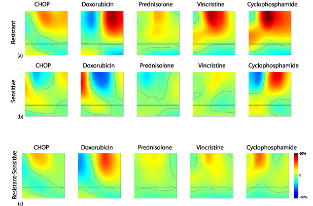
Figure 39. Drug-response spectrograms (frequency 10 mHz to 10 Hz on horizontal axis and time −4 h to 12 h on vertical axis) of canine B-cell lymphoma biopsies divided into sensitive and resistant cohorts for the combination therapy (CHOP) in addition to the individual mono-therapies.
Download figure:
Standard image High-resolution imageBacterial infections and antibiotic resistance have already become a serious health problem. The World Health Organization reports 11 million deaths per year, and bacterial resistance is predicted to become a pressing problem by 2050 when more deaths may occur from bacterial sepsis than from cancer. Bacterial infection of tissue culture is amenable to study using TDS because of the strong motions of bacteria driven by flagellar motors or by actin polymerization. An initial study of bacterial infection of DLD-1 tissues using TDS found distinct spectral signatures for Escherichia coli (E. coli) relative to Listeria monocytogenes (L. mono) and Salmonella [418]. The baseline and mid- and long-term spectra for infection by E. coli and L. mono are shown in figure 40. The E. coli infection (this strain was non-pathogenic) competes for nutrients and suppresses the metabolism of the tissue culture host. However, for L. mono infection, the listeria enters the cytoplasm of the host cells and co-opts the actin polymerization, generating fast motions that are detected as high-frequency enhancements in the spectra, as seen in figure 40(b). Antibiotic drugs were applied to strains that were sensitive or resistant to the drug, and strong responses of the bacteria to the drugs were observed, suggesting a method for testing antibiotic efficacy on a personalized-medicine basis in the case of patient sepsis screening.
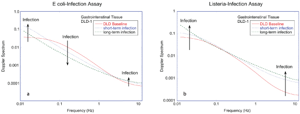
Figure 40. Experimental dynamic spectra of DLD-1 tissue culture during infection by bacteria plotting spectral density against frequency. (a) Infection by E. coli reduces the metabolic activity of the host tissue. (b) Infection by pathogenic L. mono creates strong enhancement in the organelle spectral band above 1 Hz. From [418].
Download figure:
Standard image High-resolution image5.4. Differential dynamic microscopy (DDM)
DDM is an optical microscopy technique that uses stacks of images acquired at a set frame rate, combined with Fourier transforms, to mimic DLS. Its advantages over conventional DLS include higher signal-to-noise and ease of setup (simple microscopy) [419]. The central operation is a difference between two images  separated by a time τ that removes static features while highlighting variable features that change between the two image acquisitions. When the difference images, selected by the time delay between frames, is subjected to a two-dimensional spatial Fourier transform and averaged over the time stack, the function W(k,τ) emerges as

which is similar to the function W(q,τ) at the core of DLS discussed in section 2.2. The difference arises between q and k, where q is the photon momentum transfer in DLS, while k is the transverse momentum of the particles in the DDM images. Complementary aspects of DLS and DDM include the use of coherent versus low-coherence light sources, and longitudinal versus transverse displacements, respectively. Therefore, the two techniques share much in common in analysis but are complementary in terms of transport properties for which they are respectively most sensitive. The coherent detection in DLS is sensitive to nanometer scale longitudinal motions (Doppler shifts), while the differential imaging in DDM is sensitive to sub-micron-scale transverse motions. In consequence, the characteristic times for a given transport process are much shorter for DLS than for DDM. This gives DDM an advantage when studying fast motions such as bacterial motility [420]. An additional advantage of the DDM image analysis is that the momentum k is obtained as a vector quantity rather than a single q value for a fixed scattering angle.
The physical principle of DDM is based on the stroboscopic effect with two characteristic time scales. One is the shutter speed, or exposure time, that freezes motion to within the time duration of the exposure. The other characteristic time is the time delay between subsequent acquisitions. If the change in pixel intensity occurs faster than the exposure time, then the effect is averaged out and no pixel intensity contrast is observed. If the change in pixel intensity occurs slower than the exposure time, then the motion is 'frozen' by the fast shutter speed. During the time between image acquisitions, if the change in pixel intensity is faster than the delay time, then the two frames contain different intensities and have finite differences. But if the change in pixel intensity is slower than the delay time, no difference is measured. Therefore, the rate of pixel intensity change must be faster than the slowest frame rate, but slower than the inverse exposure time (also known as the detection bandwidth). The slowest response rate is the inverse of the total time for acquiring all frames.
DDM is versatile because of its simplicity and has been adopted for a wide range of applications [421–423]. It is used primarily on optically thin 2D samples for which microscopy retains its transverse resolution. For instance, in optically thin biological samples, such as an oocyte, DDM has been used to measure intracellular motions within the cells [424]. DDM is making inroads into samples in the intermediate range of optical thickness because the limitation to quasi-2D samples can be partially overcome by confocal microscopy [425] and light-sheet microscopy [426].
5.5. Diffusing wave spectroscopy (DWS) and diffuse-correlation spectroscopy (DCS)
When light scatters multiple times in a dynamic medium, the phase shifts accumulated from each of the scattering events creates a multiple-scattering boost to the rate of the fluctuations. Light scattering in tissue is highly anisotropic, with typical anisotropy factors of g = < cosθ> ≈ 0.9, where g is the average of the cosine of the scattering angle θ, and most scattering events are small-angle forward scattering which accumulate only minimal phase shifts. This leads to a conceptual model in the moderate-scattering regime of photons that forward scatter into the tissue until they experience a high-angle back-scattering event, after which the photon again forward scatters until it leaves the medium. In this model, the majority of the accumulated phase shift is caused by the (approximately) single high-angle scattering event. Scattering lengths in translucent living tissue are typically on the order of 10 μm (about the diameter of a single cell), and the high anisotropy factor favors an extended transport length of approximately 100 μm before a high-angle scattering even occurs. Therefore, light that penetrates several hundred microns into tissue is in the moderate-scattering regime. However, light that penetrates a fraction of a millimeter or deeper into tissue is in the strong scattering regime. In this case, the light acquires a high-angle phase shift approximately every tenth of a millimeter. Light with a total propagation length of 1 mm will experience approximately 10 high-angle events, increasing the fluctuation rates by about half an order of magnitude over single-scattering rates.
In the presence of multiple scattering, DLS information can be extracted [165, 427] using DWS [166, 428–431]. The transition from moderate to deep scattering is a topic that has attracted significant effort [432–435] as well as scattering in anisotropic media [436]. Many applications of DWS involve rheology of complex media [188], as in actin filament networks [107], motor-driven dynamics in actin-myosin networks [437], and cross-linked polyacrylamide networks [438]. In biological applications, DWS has been used to assess brain activity [439, 440], to monitor blood flow [441] and the visual cortex [442] and cerebral blood flows [443]. Diffusing-wave spectroscopy can be performed with interferometric detection using long coherence [444, 445] or short coherence to resolve optical path length [434, 446–449] as well as with swept-source for coherence control [450] and with holographic detection [399, 451].
A closely related formalism for extracting dynamic information from inelastic scattering deep in tissue is DCS [104, 452–454]. Although DWS and DCS share a common physical basis, they emerged from different contexts. DCS was developed in the context of diffuse optical tomography (DOT) [455–457] that uses light scattering in the diffusion limit to perform tomographic imaging many centimeters inside tissue, while DWS is a multiple-scattering extension of QELS and often is used only up to millimeters inside tissue. In the case of DCS, the same differential equation that described the diffusive transport of spatial information in DOT also describes the transport of temporal correlations inside tissue [104]. In biological applications, DCS has been used to study tissue response to burns [458] and to monitor tissue structure [459]. It is also useful for studying blood perfusion and flow in tissues [457, 460–463]. As with interferometric DWS, DCS can be performed interferometrically [464] to measure field correlations.
5.6. Laser speckle contrast imaging (LSCI)
The dynamic imaging techniques discussed in this review have focused on in vitro or ex vivo samples in the context of biological science or diagnostics. However, a closely related light scattering technique in a clinical context is LSCI applied primarily in vivo for imaging vasculature and blood perfusion. Moving blood cells are highly dynamic targets for coherent light scattering, generating rapidly varying laser speckle in direct imaging. By measuring temporal speckle contrast in broad-area images, it is possible to create detailed maps of blood vessels in tissues.
The detection principle of LSCI is complementary to dynamic OCT and DDM. Whereas the latter two techniques rely on a short exposure time to act as a strobe, freezing the high-contrast speckle pattern within a camera frame, LSCI uses a long exposure time to average time-varying speckle to partially wash out the speckle contrast. The temporal speckle contrast is
For an exposure time T and a decorrelation time τc , the speckle contrast is [465]
where β is the instrumental contrast factor of the Siegert relation. An example of LSCI imaging vasculature is shown in figure 41. In a single speckle frame shown in figure 41(a), only slight changes in speckle contrast are observed, but in figure 41(b) the temporal speckle contrast K shows high-contrast images of vasculature under the thinned skull of a rat. Blood speeds vary by orders of magnitude from a meter per second when leaving the heart to centimeters per second in small vessels in skin to millimeters per second in capillaries. The Doppler frequency shifts (in backscatter) for these speeds range from MHz to kHz. In a transverse light-scattering geometry relevant for imaging, speckle varies over time when scatterers enter or exit a resolution volume. Assuming a resolution of 20 μm, the speckle variation rates for the same speeds are simply the inverse transit times, ranging from 50 kHz to 50 Hz. Therefore, typical exposure times to maximize the contrast in equation (5.5) for blood flow imaging is in the range of a few to tens of milliseconds.

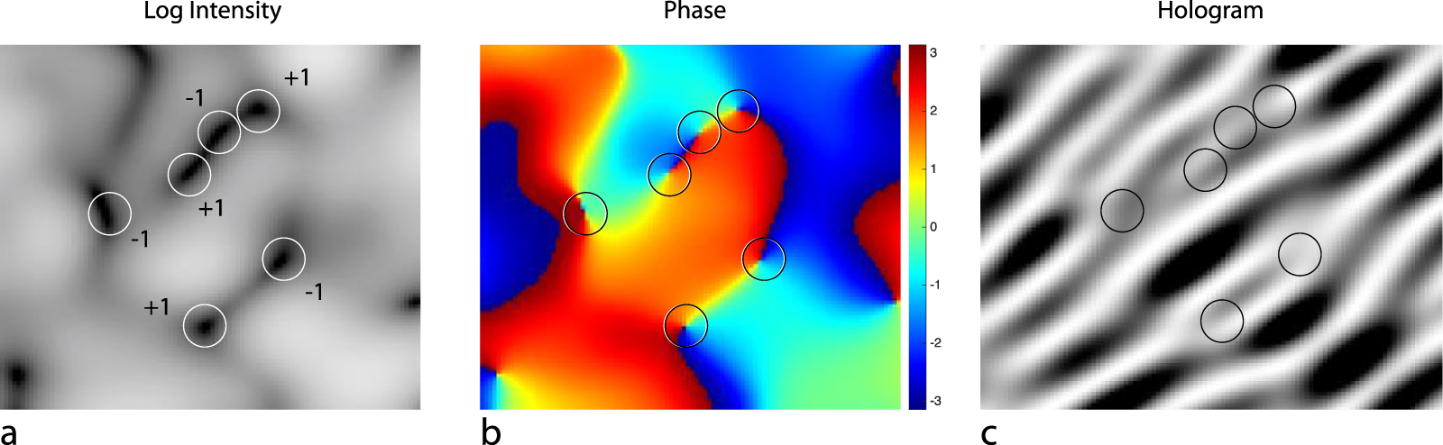
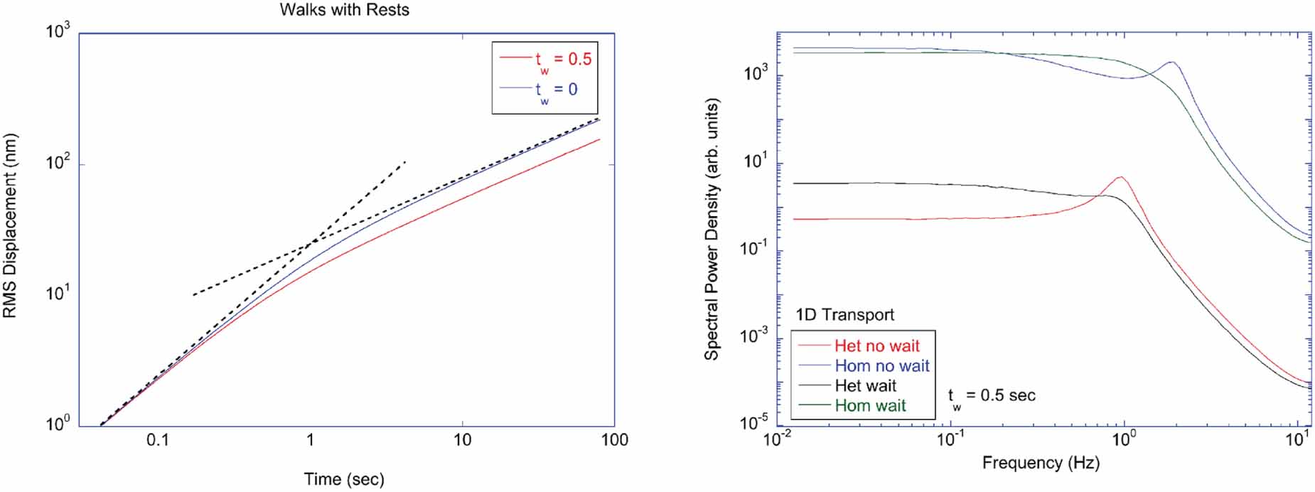
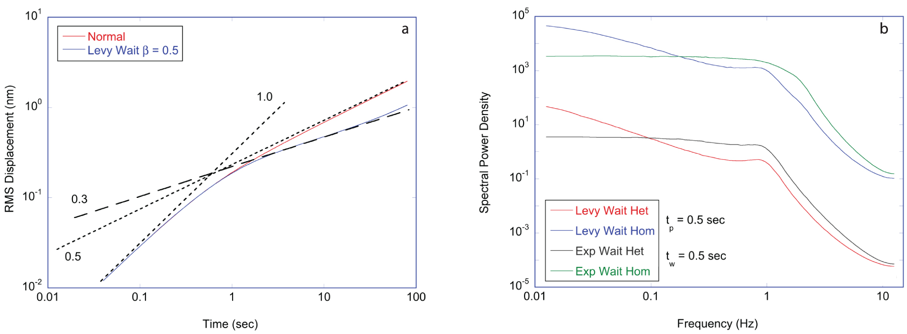
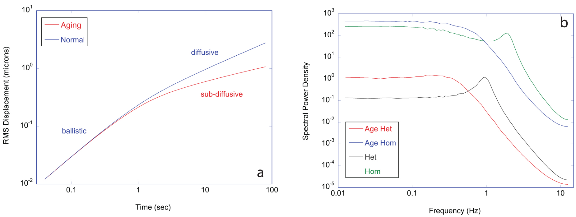
Figure 41. Laser speckle contrast imaging of the vasculature under the thinned skull of a rat. (a) A single speckle image. (b) Speckle contrast image. Reproduced from Boas et al [465]. CC BY 4.0.
Download figure:
Standard image High-resolution image
Speckle contrast imaging was first demonstrated in the 1980s but only became practical as a real-time imaging technique in the 1990s after the introduction of digital cameras to capture the dynamic speckle [330, 466–468]. Speckle contrast imaging was demonstrated in the study of cerebral blood flow in animal studies on rats [469]. The first clinical application was in ophthalmology measuring retinal microcirculation [470] followed by clinical applications in dermatology [471] for the study of burns and laser therapy of birth marks [472]. The first clinical application of speckle contrast imaging in the human brain was performed for intraoperative imaging of blood flow [473]. The technique has also been used to monitor onset of sclerosis [474] among a broadening array of further applications [475]. LSCI can be combined with DCS to perform speckle contrast optical spectroscopy [476, 477], and with OCT for depth-resolved imaging of vasculature [478, 479]. Extensive reviews are available on broad applications of speckle contrast imaging [465, 480, 481].
6. Conclusion
Macroscopic intracellular structures are driven by energetic processes that are far from thermal equilibrium, and many experience directed motion that is locally one dimensional, whether they are organelles moved by molecular motors along one-dimensional cytoskeletal tracks, or the membrane undulating primarily through local normally-directed motions. The persistence times and mean-free path lengths of these motions tend to place them within the Doppler regime for which the mean-free path length is larger than the reduced wavelength in the tissue, and the persistence times are longer than the inverse Doppler frequency shift. The Doppler spectral peaks that would result from the one-dimensional motion are not observed in light scattering experiments on tissue because the motions are isotropically oriented. Even for a single transport mechanism with a well-defined uniform speed, the projection of the motion onto the direction of the photon momentum change produces a distribution of Doppler frequency shifts with zero mean and a Doppler 'edge', also known as the knee frequency.
The Doppler edge in the side-band fluctuation power spectrum is further broadened by the distribution of speeds associated with most transport processes. Although molecular motors carrying loads can move with relatively uniform speeds under some conditions, the loads experience varying local viscosities or other impediments, and the motors can momentarily detach during a rest in motion that reduces the effective speed. Therefore, the fluctuation power spectrum is broadband and featureless and qualitatively has the diffusive form of conventional DLS. Nonetheless, remnant spectral signatures of the underlying transport processes can still be observed in the fluctuation spectra. For instance, the slope parameter for frequencies above the knee frequency depends on anomalous transport that occurs within the tissue. Ballistic or superdiffusive transport produce steeper spectral slopes, and slope exponents near or above 2 are indications of ballistic transport and the Doppler edge.
Underlying transport processes can be uncovered through perturbations of the underlying physical system. These perturbations can be from changes in the steady-state conditions of the tissue such as temperature, nutrients, osmolarity and pH. More mechanistic perturbations can use reference drugs that affect specific processes in the tissue, such as molecular motor poisons or cytoskeletal drugs that either stabilize the cytoskeleton against depolymerization or that inhibit polymerization. For instance, the cytochalasins inhibit the polymerization of actin filaments and degrade the cell cortex, lowering the bending stiffness of the cell membrane. The knee frequency itself is particularly susceptible to changes in cellular metabolism that can be affected by drugs that modify cellular energy production, such as mitochondrial uncouplers or drugs that inhibit respiration or glycolysis.
Another direction of attack to uncover underlying transport processes takes advantage of the very broad-band nature of the fluctuation spectra. Macroscopic transport processes within the cell span a dynamic range of approximately three orders of magnitude. Through a general trend imposed by the Stokes drag equation, the motions of small structures are separated in frequency from the motions of large structures, i.e. small structures move quickly, and large structure move slowly. This separates large-scale motion from small-scale motion and large-scale function from small-scale function. This separation is demonstrated in the downstream effects of some drugs, such as the induction of apoptosis by drugs that inhibit DNA synthesis. Apoptosis is a particularly energetic process with enhanced organelle transport as the cells disassemble themselves. Apoptosis also has dramatic membrane-based processes as apoptotic bodies shed off the cell. Therefore, the spectral signature of apoptosis is dominated by enhanced high-frequency spectral density (enhanced organelle transport) and by enhanced low-frequency spectral density (enhanced membrane processes) while mid frequencies are suppressed [401].
There are many outstanding problems and directions for future research exploring intracellular transport in living tissues using DLS. Continuing to connect spectral changes to direct physiological processes associated with discernible motions of subcellular constituents is an important goal of this research. Further use of reference drugs, especially that affect the mechanical properties of cells, will be useful. Cytoskeletal drugs and molecular motor drugs are among the most effective for disentangling different contributions to the fluctuation spectra. An open question is whether there are specific Doppler spectral fingerprints associated with distinct MoA. If multiple drugs with the same MoA exhibit the same or similar Doppler spectral changes, this would allow Doppler spectral measurements to rapidly and inexpensively identify new drug leads for the drug-development pipeline by classifying new compounds by their Doppler-associated MoA.
One of the biggest outstanding challenges is to connect spectral changes to alterations in the underlying intracellular signaling pathways. Genetic profiling methods such as RNA sequencing will be an important future tool to achieve this goal. Drugs that affect signaling pathways modify the expression of relevant RNA that can be sampled from tissues that have been interrogated using Doppler FS. This would allow modified spectral changes to be connected with modified protein expression. Once these connections are established and calibrated, it could allow DLS to stand in, when appropriate, as a low-cost surrogate for RNA-seq methods currently in use for drug screening and drug development. This also can help move Doppler spectroscopy into personalized cancer care. When a drug fails to affect the targeted signally pathway, verified by RNA-seq, there may be an associated Doppler drug-response signature. In this case, subsets of a patient cohort who are resistant to a prescribed therapy may be identified rapidly by Doppler profiling, as a chemoresistance test, and directed to more effective therapy.
Within chemoresistance testing using Doppler profiling, an important question is whether there are 'universal' Doppler signatures across multiple diseases, multiple tissue types and multiple drugs. Currently, every new cancer indication and treatment option requires a separate pilot clinical trial to establish the Doppler drug-response profiles against which future patients are classified. Clinical trials are lengthy and expensive. If universal Doppler profiles emerge along the lines of common MoA for a range of different drugs on different cancers and tissue types, then expanding the use of Doppler profiling to new diseases and new drugs (with known MoA) may not require separate clinical trials, but trial results could be pooled across diseases and drug MoAs, accelerating the adoption of Doppler profiling for personalized therapy selection.
More and larger clinical trials of Doppler profiling are still be needed to better understand the origins and role of biological variability and the effect on individual and averaged Doppler profiles. Clinical biopsy specimens tend to have highly heterogeneous structure and tissue constituents such as stromal tissue and fat mixed in with epithelial tissues and cancerous tissues. This mixture of tissue types within a single interrogated specimen presents a challenge to interpretation because different tissue constituents may respond differently to applied drugs. TDS imaging (as discussed in section 5.4) may help disentangle signatures, but in addition to the spatial heterogeneity, there is also the genetic heterogeneity of cancer biopsies. The varying genotypes within an interrogated sample may yield varying phenotypes. The effects of such intra-specimen phenotypic variability on patient chemosensitivity classification must be explored further. On the other hand, this very heterogeneity may be exploited using neural networks such as deep encoders to improve prediction of patient chemosensitivity. For instance, the heterogeneous signatures from a single patient may have nonlinear or linearly non-separable relationships to the patient's response to a selected therapy. Retaining the heterogeneity in the Doppler drug responses, rather than averaging over the varying signatures, may provide important signal channels for deep encoder approaches that reduce the dimensionality of the prediction problem to predict patient likelihood of responding to a treatment.
From an optical development perspective, there are challenges in the design and construction of apparatus to extract the Doppler drug profiles. Some of the current dynamic OCT systems rely on on-axis or off-axis digital holography in Mach–Zehnder or Michelson configurations that are sensitive to mechanical disturbances. Common-path interferometer systems are much less susceptible to mechanical disturbances [482], but many common-path interferometer designs are not compatible with low-coherence light sources. Combining low-coherence with common-path designs is an open design problem that may have many possible solutions, leading to stable and compact interferometric systems that can be used at the point-of-care. There is also a potential role for adaptive optics to enable deeper penetration of light into the highly-scattering tissue samples while also achieving improved spatial resolution. Of particular importance is the potential to compensate for the 'shimmering shower glass' effect where overlying layers of dynamical motions affect the spectra of underlying layers that are captured within the coherence gate. Additional challenges remain in the extraction of dynamical contrast from OCT systems. Current approaches to OCT emphasize spatial resolution of structure that is incompatible with strong speckle needed for speckle FS. Either a balance must be set between structural resolution and spectral dynamic range, or the current trade-off must be broken by a new design principle that would allow high-dynamic-range spectra to be superposed on high-spatial-resolution images.
Because life and motion are so intimately connected—life is literally animated—experimental techniques that access and differentiate the wide diversity of intracellular and tissue motions would have significant impact on the growing understanding of life and disease. Light is an ideal probe to use for this challenge by providing a means to convert motion into optical signals. Optical interferometry of partially coherent light, even within the highly scattering context of living tissue, is sensitive to a wide dynamic range of motion from the nano-scale to the micro-scale. Interferometric imaging is also compatible with large field of view, retaining its sensitivity down to nano-scale motion while interrogating millimeter-scale specimens of living tissue. The nano-scale sensitivity, combined with high dynamic range and wide field of view, holds promise for expanded uses of light scattering from intracellular transport in living tissues.
Acknowledgments
This research is supported by NSF Grant CBET-2200186.
Data availability statement
The data that support the findings of this study are available upon reasonable request from the authors.