
Abstract
This paper extends a 1D dynamic physics-based model of the scrape-off layer (SOL) plasma, DIV1D, to include the core SOL and possibly a second target. The extended model is benchmarked on 1D mapped SOLPS-ITER simulations to find input settings for DIV1D that allow it to describe SOL plasmas from upstream to target—calibrating it on a scenario and device basis. The benchmark shows a quantitative match between DIV1D and 1D mapped SOLPS-ITER profiles for the heat flux, electron temperature, and electron density within roughly 50% on: (1) the Tokamak Configuration Variable (TCV) for a gas puff scan; (2) a single SOLPS-ITER simulation of the Upgraded Mega Ampere Spherical Tokamak; and (3) the Upgraded Axially Symmetric Divertor EXperiment in Garching Tokamak (AUG) for a simultaneous scan in heating power and gas puff. Once calibrated, DIV1D self-consistently describes dependencies of the SOL solution on core fluxes and external neutral gas densities for a density scan on TCV whereas a varying SOL width is used in DIV1D for AUG to match a simultaneous change in power and density. The ability to calibrate DIV1D on a scenario and device basis is enabled by accounting for cross field transport with an effective flux expansion factor and by allowing neutrals to be exchanged between SOL and adjacent domains.
Export citation and abstract BibTeX RIS

Original content from this work may be used under the terms of the Creative Commons Attribution 4.0 license. Any further distribution of this work must maintain attribution to the author(s) and the title of the work, journal citation and DOI.
1. Introduction
The development of commercial fusion reactors greatly depends on models to evaluate designs prior to their construction [1]. A major challenge is the design and control of the heat exhaust—to handle the enormous heat and particle fluxes that flow from the main plasma/core into the exhaust (called divertor) [2, 3]. To guide control system designs, the dynamics governing these heat and particle fluxes must be modeled [4]. One of the modeling efforts is the 1D dynamic model of the divertor plasma called DIV1D [5]. This model was recently benchmarked on static 2D scrape-of-layer (SOL) plasma simulations of the established SOLPS-ITER edge model [6] showing good agreement below the X-point [7].
As a logical next step, this paper extends and validates the DIV1D code [7] to above the X-point—beyond the outer midplane [8]—up to the stagnation point. We validate the DIV1D code on SOLPS-ITER simulations not only for Tokamak Configuration Variable (TCV), but now also for Upgraded Mega Ampere Spherical Tokamak (MAST-U) and Upgraded Axially Symmetric Divertor EXperiment in Garching Tokamak (AUG). In essence, the 1D mapping of 2D SOLPS-ITER for the divertor plasma in [7] is extended to the core SOL (core-sol) and used to calibrate DIV1D such that it self-consistently recovers SOL plasma solutions from target to stagnation point on a scenario and device basis.
The remainder of the paper is structured as follows. The extension of DIV1D with a core-sol is described in section 2. The main heat flux channel is used to map 2D SOLPS-ITER solutions to 1D and extract boundary conditions and settings for DIV1D in section 3. The DIV1D simulations are calibrated on and compared to 1D mapped SOLPS-ITER solutions for TCV, AUG, and MAST-U in section 4. Results are discussed in section 5.
2. Extending DIV1D to the core-sol
The DIV1D model is based on the assumption that in the SOL parallel plasma transport dominates cross-field transport. Consequently the domain can be represented in a set of balance equations along the magnetic field B for the respective plasma density, momentum, and energy as well as for the atomic neutral density:

The plasma electron density n, parallel ion velocity  , ion and electron temperature T and atomic neutral density
  are solved along coordinate x. The static plasma pressure
  , parallel plasma particle flux
  , momentum flux
  and heat flux
  follow from definitions. For the heat flux a parallel conductivity is taken as
  (see chapter 4.10.1 of [9]). The electron charge e and mass of the main ion species m are constants—in this work we consider deuterium. Details on the neutral diffusion coefficient D and the source terms
  can be found in [7]. One particular addition is a finite neutral energy
  in the energy source:

where the effective charge exchange and ionization source of neutral energy respectively follow from their volumetric rates  and
and  . The energy is converted to SI units with the elementary charge
  . The neutral energy is set to
  throughout this work, this is equivalent to a neutral temperature of
  . On the other hand, the neutral diffusion coefficient, is set only by the ion temperature T and not by a harmonic average with the neutral temperature
  . The rationale being that neutrals equilibrate with the plasma when they diffuse along the SOL. It is important to note that molecules are not considered in DIV1D for simplicity, but that molecules are expected to have a significant influence on solutions [10, 11].
Similar models have been implemented by various authors in their respective 1D codes [12–16] and seem to focus on evolving the equations in single (magnetic) flux-tubes. For reasonable descriptions of the full divertor heat flux channel in 1D, the key contribution of DIV1D in [7] was accounting for cross-field channel widening (using an augmented magnetic field strength) such that the plasma balance equations feature no radial losses on the DIV1D domain. Another contribution was to allow for neutral transport between the SOL and external gas reservoir through a particle exchange timescale. In the SOL, this addition resulted in a neutral source upstream and a neutral sink in front of the target.
The domain of DIV1D is extended—with respect to [7]—to include the full core-sol and a second divertor SOL (div-sol) with second target. For this work, however, we focus on simulations with a single target and imply zero flux (Neumann) boundary conditions at the point where the ion flow reverses direction. The stagnation point forms a natural boundary between solutions of different divertor legs. Due to the zero-flux boundary condition, the solution of DIV1D is governed by fluxes from the core and interaction with the neutral gas reservoir(s). The following sections detail the added features in geometry, boundary conditions, sources and sinks.
2.1. Geometry
To enable quantitative interactions between the SOL and external domains, geometric properties are defined on the grid of DIV1D along the principle x direction. As a basis for the geometric description we define the following invariant for heat flux conservation:

where  is the poloidal SOL width and
  is the inclination angle given by the poloidal over the toroidal magnetic field. The expansion of the heat flux channel described by DIV1D (
 governing B in [7]) is split into a contribution from the magnetic field
  and one that is used to mimic cross-field transport
  , see examples of cross-field transport in [17]. In this way, when
  remains unchanged the transport field
  can still widen the poloidal SOL width
  . The area
  of cells
 ![${i \in [1,N]}$](https://content.cld.iop.org/journals/0741-3335/66/5/055004/revision2/ppcfad2e37ieqn25.gif) in contact with external domains along the poloidal direction, but not at the target/stagnation plane, is approximated as follows:
in contact with external domains along the poloidal direction, but not at the target/stagnation plane, is approximated as follows:

where the length of cells  parallel to the magnetic field is projected poloidally with the pitch angle
  and multiplied with the circumference of the plasma
  at the cell location xi
. The cell volumes Vi
follow from multiplication:
at the cell location xi
. The cell volumes Vi
follow from multiplication:

The extended DIV1D geometry requires additional information on the inclination angle  , major radius R, and cross-field widening of the heat flux channel (mimicked in the transport field
  ). The transport field
  is set through the transport expansion coefficient
  starting from the X-point location LX
up to the target with connection length L:
starting from the X-point location LX
up to the target with connection length L:
The magnetic field strength  and
and  together define the magnetic equilibrium of DIV1D, where the magnetic field
  can be given as a vector input to DIV1D or set through the magnetic flux expansion factor εB
, by substitution in equation (9). The field B as used in the equations of DIV1D is obtained by multiplication of magnetic and transport effects:
can be given as a vector input to DIV1D or set through the magnetic flux expansion factor εB
, by substitution in equation (9). The field B as used in the equations of DIV1D is obtained by multiplication of magnetic and transport effects:  . The external area
  and volumes V are calculated on cell centers, other quantities
  ,
,  , B, and R are also calculated on cell faces.
2.2. Boundary conditions
The boundary conditions at the upstream point are considerably more simple. The upstream boundary is now given by a stagnation point where all fluxes are set to zero. i.e. the plasma heat  , velocity
  and neutral density derivative
  are set to zero. The target boundary conditions remain unchanged with respect to those in [7]. Although not used in this work, DIV1D also supports simulation of the full SOL from target to target using sheath boundary conditions at both ends of the domain and core-flux source terms in the core-sol.
2.3. Sources and sinks
The upstream boundary condition no longer allows any particle, momentum, or heat fluxes to enter the DIV1D domain. Instead the fluxes established at the X-point originate from the core and vacuum external to the SOL. The flux of external neutrals into the SOL is determined as:

where the cross-tube neutral flux  follows from the difference between external gas density
  and neutral SOL density nn
, multiplied with the external area
and neutral SOL density nn
, multiplied with the external area  and an exchange velocity
  . The external gas density can be defined for both the core and divertor common flux region (CFR), as well as for the divertor private flux region (PFR). We note that
  replaces the neutral exchange time
  in [7]. The external neutral gas density
  for the divertor and core region can be set independently to mimic density differences caused by baffles. Similarly different values can be specified for the CFR and PFR.
The cross-sol neutral flux enters the div-sol from both the PFR and CFR. As such the div-sol neutral source is determined by:

where fluxes are doubled (with for simplicity equal neutral density in PFR and CFR) and divided by the volumes V. For the neutral flux into the core-sol it is noted that a large fraction  can propagate into the core before being ionized, reducing the neutral source in the core-sol as follows:

The plasma sources that originate from the core are calculated using the total core heat and ion fluxes ![$\Gamma_\mathrm{core}~\mathrm{[ s^{-1}]}$](https://content.cld.iop.org/journals/0741-3335/66/5/055004/revision2/ppcfad2e37ieqn51.gif) and
and ![$Q_\mathrm{core}~\mathrm{[J\,s^{-1}]}$](https://content.cld.iop.org/journals/0741-3335/66/5/055004/revision2/ppcfad2e37ieqn52.gif) , respectively. These fluxes are multiplied with a normalized spatial profile. This core source spatial profile is calculated as:
, respectively. These fluxes are multiplied with a normalized spatial profile. This core source spatial profile is calculated as:

This is normalized to  where the integral
  equals unity. The profile shaping parameter α can be used to shape the distribution and create peaked or flat profiles, enabling varying flux distributions over the seperatrix due to different (neoclassical or anomalous) transport phenomena. Multiplication with the area
  in the normalized distribution allows direct division with volumes to obtain volumetric sources for heat and particles (respectively
  and
and  ) as follows:
where the flux distributions  are equal for particles and heat. It is noted that ionized particles leave the core-sol as they flow into the far SOL (far-sol). This far-sol sink is omitted in the DIV1D equations as we enforce all ion fluxes to be redirected into the divertor. This is contrary for neutral cross-channel transport as set by the core-ionization fraction
  and exchange velocity
  . The sources are considered in the main equations of DIV1D according to their subscripts, e.g.
  is added to the right hand side of the energy balance. The superscripts div and core denote if the source takes effect in the divertor or core-sol.
The goal for DIV1D is to produce realistic SOL solutions as function of core fluxes and external neutral densities. In order to systematically test DIV1D, the following section investigates the main SOL heat flux channel based on 2D solutions of SOLPS-ITER.
3. The SOL in 1D based on 2D SOLPS-ITER simulations and extracting settings for DIV1D
In this section we map the SOL from SOLPS-ITER to a 1D heat flux channel profile and use this to extract sources and sinks from external domains. The SOLPS-ITER code package uses the B2.5 plasma solver supported by EIRENE for kinetic neutral solutions or fluid neutrals from an internal package [18]. The SOLPS-ITER simulations considered in this work are from the TCV [6], AUG [19], and the MAST-U [20]. Except for MAST-U these SOLPS-ITER simulations have been extensively compared to experimental data in the respective papers. It is noted that in those papers, simulation settings are typically changed to align SOLPS-ITER with experimental measurements—e.g. of heat fluxes, ion and electron temperatures, neutral pressures—providing a physics-based interpretation of considered experiments.
The poloidal B2.5 grid is depicted in figure 1 for TCV, MAST-U and AUG. It can be seen that the B2.5 grid is aligned with the magnetic field in y and perpendicular to the magnetic field in x. One can also use figure 1 to compare the scale of the devices, most notably the divertor plasma of MAST-U that extends all the way to the major radius of AUG. The following subsections focus on the SOL in the B2.5 grid to identify the main heat flux channel and study the sol-core interaction through cross-channel fluxes.

Figure 1. The B2.5 grid from SOLPS-ITER simulations of the edge plasma in TCV, MAST-U, and AUG. The x-coordinate is perpendicular to the magnetic field and the y-coordinate is aligned with the magnetic field.
Download figure:
Standard image High-resolution image3.1. The main heat flux channel
In this work, 1D SOL equilibria always represent the main heat flux channel and not single flux tubes. Due to cross-field transport, solutions of single flux tubes are unlikely to reflect macroscopic divertor plasma behavior [7]. This is illustrated in figure 2 where the full width at half the maximum (FWHM) of the heat flux [7] denotes the main heat-flux channel on the B2.5 grid coordinates (i.e. along grid cells x and y in figure 1). In figure 2, a dashed dotted line indicates the peak heat flux location. Along y toward the target, it can be seen that the channel widens in x and that the peak heat flux drifts radially outwards to larger x. Both effects are not captured by a single flux tube, while they are by the main heat flux channel. In the following paragraphs we discuss how the heat flux channel mapping is extended into the core-sol.
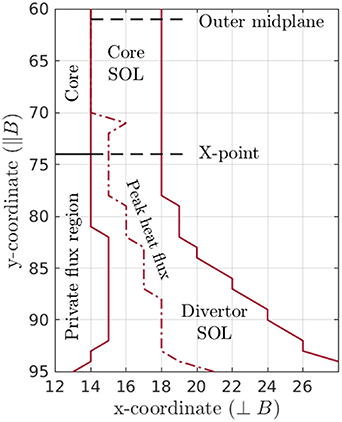
Figure 2. The main heat flux channel on the B2.5 grid for SOLPS-ITER simulation #150 683 for TCV. In the core-sol, the heat flux channel is bounded by the seperatrix and fixed in width. Toward the X-point, the peak heat flux—denoted by the dashed dotted line—moves away from the seperatrix and drifts radially outward below the X-point. In the divertor SOL the inner and outer bounds of the main heat flux channel are located around the 50% decrease of parallel heat flux with respect to the peak heat flux, the FWHM.
Download figure:
Standard image High-resolution imageIn the core-sol the solutions are mainly determined by the perpendicular fluxes from the core. For example, the stagnation point is a result of the distribution of perpendicular core fluxes. Near the stagnation point parallel fluxes even become multi-directional, e.g. in the poloidal plane the bulk particle flow close to the seperatrix is down and further outward the bulk flow is up. To reduce the impact of multi-directional parallel fluxes and perpendicular flux distributions, we select a fixed number of B2.5 grid cells in the core-sol to represent the main heat flux channel (see also figure 2). The number of radial grid cells is chosen to align with the FWHM of the heat flux distribution just below the X-point, to circumvent 2D effects around the X-point [7]. Similar to [7], the main heat flux channel is used to map 2D SOLPS-ITER solutions of the SOL to 1D profiles along the leg. Along the x-coordinate in B2.5, the average, minimum and maximum values of quantities in the heat flux channel are used to construct 1D profiles along the leg (y-coordinate) where the extreme values represent lumped value intervals. It is noted that the mean values might not conserve physical quantities inside the selected regions of interest, e.g. internal energy. This 1D mapped SOLPS-ITER representation with fixed core-sol width and FWHM divertor-sol is used to inform DIV1D simulations and compare DIV1D with SOLPS-ITER in the remainder of this paper.
3.2. Cross-channel fluxes
In this section we use the SOLPS-ITER solution of TCV simulation 150 683 to investigate the global heat and particle balances in the core-sol. Particularly interesting as boundary conditions for DIV1D are the fluxes that enter the core-sol over the seperatrix and leave into the far-sol. In literature the far-sol is typically denoted by changes in decay lengths and types of transport [21]. In this work the distinction between near SOL (near-sol)/core-sol and far-sol is not based on fundamental theory such as presented in [21], but simply by the domain that is averaged to obtain 1D profiles of plasma quantities from SOLPS-ITER.
In figures 3 and 4 the respective heat and ion particle flux over the seperatrix (SEP inflow) into the core-sol are depicted together with the outflow into the far-sol (far-SOL outflow). The distance to the target covers the core-sol from stagnation point to X-point, from 18 m to 8 m respectively. It can be seen that a large fraction of the fluxes that flow into the near-sol also flow out to the far-sol. The fraction of ions that flow out to the far-sol is larger than the fraction of heat flowing to the the far-sol. This is likely because the decay length for heat is smaller than for density [21]. Additionally, large fluxes can be observed near the X-point. Finally it is noted that, despite the large outflow into the far-sol, the majority of heat flows into divertor through parallel transport. The following subsection uses the heat flux channel mapping to determine inputs/settings for DIV1D.

Figure 3. Cross-channel heat fluxes for the core scrape-off layer as function of distance to target, taken from SOLPS-ITER simulation 150 683. SEP inflow denotes the heat flux over the seperatrix and far-SOL outflow denotes the heat flux flowing radially out of the main heat flux channel into external neutral gas reservoir.
Download figure:
Standard image High-resolution image
Figure 4. Cross-channel particle fluxes for the core scrape-off layer as function of distance to target, taken from SOLPS-ITER simulation 150 683. SEP inflow denotes the particle flux over the seperatrix and far-SOL outflow denotes the particle flux flowing radially out of the main heat flux channel into external neutral gas reservoir.
Download figure:
Standard image High-resolution image3.3. Selecting DIV1D settings
The goal for DIV1D is to obtain realistic target and upstream SOL plasma quantities as function of core-fluxes (e.g. from core codes) and external neutral reservoir densities. In this section we extract settings for DIV1D from 1D mapped SOLPS-ITER solutions given that the main heat flux channel has a fixed number of B2.5 grid cells that define the width of the core-sol.
- The heat and particle sources from the core—Qcore and
 —are obtained from the integral of cross-channel fluxes into the main heat flux channel as displayed in figures 3 and 4. The fluxes into the far-sol are not considered because a majority of these particles is still transported into the divertor. Also the majority of the heat is found to be transported into the divertor.
 - The geometric values for and R can be specified separately in the div-sol and core-sol. The values are obtained by the average of the mapped 1D SOLPS-ITER profiles in the respective domains. Alternatively single values are used or full arrays are interpolated on the DIV1D grid.
- The transport field is extracted from SOLPS-ITER solutions by comparing the area of the heat flux channel in front of the target and just below the X-point while correcting for the contribution of magnetic flux expansion.
- The poloidal SOL width is constructed by setting a value around the outer midplane and augmenting this with the transport field and magnetic pitch angle (i.e. following equation (6)).
- The core ionization fraction is used as a fitting parameter, and expected to be related to the ratio between the ionization mean free path and poloidal SOL width .
- The neutral exchange velocity is a fit parameter that is expected to have the order of magnitude of the neutral thermal velocity.
- The external neutral reservoir density is obtained by averaging over the outer B2.5 cells for the core-sol and div-sol. This is an important difference with respect to [7], where the median value of the neutral particle density inside the SOL was selected. Another important remark is that in this work an effective neutral density is taken as only the atomic density.


A detailed list of (expected) DIV1D settings extracted from SOLPS-ITER for this paper is available in appendix  ; and the neutral exchange velocity
  . The following section utilizes DIV1D settings as derived from mapped SOLPS-ITER solutions to simulate the SOL in 1D on multiple devices.
4. Comparison of DIV1D simulations to mapped 1D profiles from SOLPS-ITER for TCV, AUG, and MAST-U
In this section we aim to demonstrate that the core-sol extension of DIV1D allows it to describe the SOL plasma from target up to the stagnation point. To this end—after extracting DIV1D settings from 1D mapped SOLPS-ITER solutions—we use the three parameters  ,
,  , and
, and  to calibrate DIV1D on 1D mapped SOLPS-ITER simulations of TCV, AUG, and MAST-U. The SOLPS-ITER simulations on TCV [6] and AUG [19] where compared to experimental data in respective publications. The most important inputs for DIV1D simulations of the devices are presented together in table 1. The following sections explain how these values are obtained with a calibration procedure and further cover the 1D simulations with DIV1D on these devices.
Table 1. Characteristic inputs of DIV1D simulations for TCV, AUG, and MAST-U, after aligning with  , and
, and  . For starred
  values full arrays are used. The origin of stated values is described in appendix
| Setting | R |

|

|

|

|

| εB |

|

|

|

|
|---|---|---|---|---|---|---|---|---|---|---|---|
| TCV | 0.95
| 0.05
| 10 | 8 | 270 | 2.1 | 1.1
| 2.3
| 0.015 | 3800 | 0.8 |
| AUG | 1.8 | 0.035 | 25 | 10 | 700–830 | 1.1 | 1.06 | 1.17 | 0.05–0.15 | 555 | 0.6 |
| MAST-U | 0.97 | 0.05 | 5.8 | 23.1 | 1250 | 3 | 2.7 | 8.1 | 0.077 | 1000 | 0.9 |
| Unit | (m) | (—) | (m) | (m) | (kW) | (—) | (—) | (—) | (m) | (m s−1) | (—) |
4.1. TCV
For the TCV the DIV1D model with core-sol is evaluated on a set of SOLPS-ITER simulations from [6] that represent a density ramp (see figure 5 in [7] where the same set of simulations was used). These SOLPS-ITER simulations are extensively compared to experiments in [6]. The inputs for DIV1D that follow from SOLPS-ITER simulations are as follows: core-sol length  ; div-sol length
  ; transport expansion
  ; a homogeneous carbon concentration
  , and heat flux from the core
  distributed with α = 1 following equation (13). Geometric descriptions of pitch angle
  , major radius R, magnetic field strength
  are arrays taken from mapped SOLPS-ITER profiles along the SOL. Neutral densities in reservoirs adjacent to the core and divertor (PFR and CFR) depend only on the atomic density in the edge of the B2.5 grid in SOLPS-ITER simulations. Detailed values are listed in table A1.
A number of parameters are chosen to match DIV1D with 1D mapped SOLPS-ITER heat flux channel profiles. The core-sol width is chosen at  to match the accumulated parallel heat flux at the X-point. The core ionization fraction
  was used to match the upstream density and the neutral exchange velocity
  was used to obtain agreement in the div-sol profiles. Target recycling is set as
  to reduce the target neutral density. Even though the same SOLPS-ITER solutions were used as in [7], the input parameters for DIV1D were changed in two ways in this work: (1) the neutral exchange velocity was changed; (2) the neutral reservoir density is here taken at the boundary of the B2.5 grid where in [7] one takes the median of the atomic density inside the SOL.
Results on three simulations in a density ramp for high-recycling conditions are presented in figure 5, where DIV1D is depicted together with SOLPS-ITER. It can be seen that the profiles for heat flux  , temperature T and electron density
  of SOLPS-ITER and DIV1D are similar with DIV1D often laying inside the value intervals of the 1D mapped SOLPS-ITER solutions. The neutral atom density
  of DIV1D lies close to the value intervals from the X-point up to a few meters in front of the target, but is very different in the core-sol. Another large discrepancy is observed in the parallel velocity where DIV1D overestimates the velocity by up to 10 km s−1. Also notable is that the temperature of ions and electrons in the core-sol is not the same in SOLPS-ITER and that DIV1D is consistently close to the electron temperature.

Figure 5. Comparison between DIV1D and SOLPS-ITER (simulations: #150 678, #150 683, #150 688) for a density ramp in high recycling conditions increasing from left to right. The simulation domain ranges from outer target to the stagnation point where the X-point is located around 8 m to the target. On display are the parallel heat flux  , temperature T, electron density
  , parallel ion velocity
  , plasma neutral atom density
  . For DIV1D, the densities of the external gas reservoirs are represented as dashed lines
  . The SOLPS-ITER profiles have value intervals representing the minimum and maximum values inside the main heat flux channel that was mapped to 1D solutions along the leg.
Download figure:
Standard image High-resolution imageAdditionally, we compare the upstream electron density  and temperature
  of DIV1D to that of SOLPS-ITER. Figure 6 depicts the upstream density as function of neutral density in the divertor CFR gas reservoir
  . It can be seen that the trend of DIV1D is similar to that of SOLPS-ITER although DIV1D underestimates the upstream density
  by roughly 20% for the neutral densities
  above
above  . In figure 7 the outer midplane (upstream) temperature
  versus upstream electron density
  is compared for 1D mapped SOLPS-ITER and DIV1D heat flux channel solutions. It can be seen that DIV1D temperatures are inside the value interval of electrons in 1D mapped SOLPS-ITER.

Figure 6. Comparison of upstream outer midplane (omp) electron density  as function of external density of the divertor CFR gas reservoir
  for 1D mapped SOLPS-ITER and DIV1D.
Download figure:
Standard image High-resolution image
Figure 7. Comparison of upstream outer midplane (omp) temperature  as function of upstream electron density
  for 1D mapped SOLPS-ITER and DIV1D.
Download figure:
Standard image High-resolution image4.2. AUG
For the AUG tokamak we calibrate the DIV1D model on three SOLPS-ITER simulations reported in [19]. These simulations represent divertor plasmas from the onset of detachment to complete detachment and are validated on experimental discharges #27 100 and #34 821. The inputs for DIV1D again follow from mapping SOLPS-ITER solutions, with detailed values given in table A2. The most important settings of DIV1D include a power of roughly  , no impurities, small flux expansion
  and very small transport based expansion
  . Geometrical parameters are set as: connection length
  , div-sol length
  ,
,  , and major radius
  . Interesting to note is that both heat and particle fluxes over the seperatrix change between simulations and the core-sol widens. These varying parameters are listed in table 2 along with changes in the external neutral gas reservoir density in the PFR as extracted from SOLPS-ITER solutions.
Table 2. Important settings of DIV1D for the comparison for AUG in figure 8
| MDS |

|

|

|

|
|---|---|---|---|---|
| 182 202 | 0.6 | 703 | 1.1 | 0.05 |
| 182 203 | 0.9 | 719 | 4.6 | 0.08 |
| 182 204 | 1.3 | 835 | 7.3 | 0.15 |
| Unit |

| (kJ s−1) |

| (m) |
To calibrate DIV1D, we select the SOL width  to match the X-point heat flux. To match the particle balance we chose the neutral exchange velocity
  ; target recycling
  ; and core ionizing fraction
  . The varying inputs for the DIV1D simulations are listed in table 2. Note here that we vary the SOL width
  beyond the values found from 1D mapped SOLPS-ITER. Equally important is that we list the change in PFR neutral density for these SOLPS-ITER simulations as the neutral density in the PFR exceeds that in the CFR as a result of the vertical targets in these AUG experiments. In SOLPS-ITER this neutral balance is tuned to roughly match experiments by introducing artificial baffling and pumping to mimic the changing neutral transport characteristics during a discharge, e.g. because the wall transitions from a sink to a source [22].
Varying the setting for the midplane SOL width, results of three DIV1D simulations for AUG are depicted in figure 8 ranging from attached to detached divertor plasmas. The attached state can be recognized in simulation  182 202 by the high target temperature (
 ) that relates to a high target velocity and low recycling. This low-recycling relates to the drop in electron density near the target. For details relating to the detachment state the reader is referred to [11, 23] and references therein. There are two distinguishable dashed blue lines for
  in the divertor below the X-point where the high and low value respectively represent the PFR and CFR atomic neutral density as used in the DIV1D simulation. Compared to the mapped SOLPS-ITER solutions, it can be seen that DIV1D matches the electron temperature. Whereas the ion temperature is consistently higher in the core-sol. The parallel heat flux of DIV1D also closely follows SOLPS-ITER. The connection length of DIV1D was set constant across simulations while the connection length of 1D mapped heat flux channel profiles varied from 36 to 32 m. Consequently one can observe local minima in the heat flux around 33 m for #182 203 and #182 204. Finally, it can be seen that DIV1D overestimates the velocity around the X-point and that DIV1D overestimates the upstream electron density in #182 202. This could be due to drift effects, see e.g. [24], not considered in DIV1D [7].

Figure 8. Comparison between DIV1D and SOLPS-ITER (simulations: #182 202, #182 203, #182 204) for a simultaneous density and power ramp increasing from left to right. The simulation domain ranges from outer target to the stagnation point where the X-point is located around 9 m to the target. On display are the parallel heat flux  , temperature T, electron density
  , parallel ion velocity
  , plasma neutral atom density
  . For DIV1D, the densities of the external gas reservoirs are added as dashed lines
  , it is noted that the density outside the scrape-off layer can be different in private flux region and common flux region—which is the case here resulting in two dashed blue lines below the X-point.
Download figure:
Standard image High-resolution image4.3. MAST-U
For the MAST-U tokamak, DIV1D is calibrated on SOLPS-ITER simulation #67 989 from [20]. This simulation represents an L-mode high power edge plasma for a double-null configuration with a super-X tightly baffled divertor geometry. Unfortunately it has not been compared to experimental data yet in [20]. Again, most inputs for DIV1D are set using the 1D mapped SOLPS-ITER solution of the main heat flux channel.
For the MAST-U simulation we use the following base settings: a power of  , carbon impurity concentration
  , flux expansion
  and transport expansion
  . The geometry is defined by a connection length
  , div-sol length
  ,
,  , and major radius
  . The large change in major radius toward the target is expressed in the flux expansion
  and causes significant changes in the value of the field B in the DIV1D equations. It is also noted that the very detached equilibrium of MAST-U divertor plasmas obstruct the derivation of transport expansion
  from 1D mapped SOLPS-ITER solutions, consequently this value is relatively uncertain compared to those found for TCV and AUG.
The process of calibrating DIV1D on SOLPS-ITER simulations of MAST-U is similar to that on TCV and AUG. Firstly, changing the SOL width  to match the X-point parallel heat flux
  . Secondly, adapting the neutral exchange velocity
  and core ionization fraction
  to adjust the particle balance. Target recycling is set to
  , but solutions are not very sensitive to this parameter in the considered simulation.
The resulting calibrated DIV1D simulation for MAST-U is depicted together with the corresponding 1D mapped SOLPS-ITER heat flux channel solution in figure 9. It can be seen that the temperature T and parallel heat flux  lie almost within the value intervals of the SOLPS-ITER solutions. On the other hand, the plasma density
  is over-predicted between 26 and 20 m to the target while the parallel velocity
  is under-estimated by DIV1D.
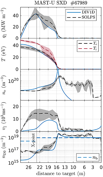
Figure 9. Comparison between DIV1D and SOLPS-ITER simulation #67 989 for MAST-U. The simulation domain ranges from lower outer target to the stagnation point where the X-point is located around 23 m from the target. Depicted are the parallel heat flux  , temperature T, electron density
  , parallel ion velocity
  , plasma neutral atom density
  . For DIV1D, the densities of the external gas reservoirs are added as dashed lines
  .
.
Download figure:
Standard image High-resolution imageA highlight for the MAST-U super-X divertor is the volumetric recombination region, which can be seen from 14 m to the target as a peak and decay in the plasma density  . As the temperature T falls below 0.5 eV, recombination becomes a dominant sink in DIV1D causing the plasma density
  to reduce two orders of magnitude—ending below
  whereas the solutions of SOLPS-ITER ion densities remain above
  .
.
4.4. Discussion
In previous work on validating DIV1D in [7] the domain was constrained to a region below the X-point. The reason was that the X-point plasma quantities in 1D mapped SOLPS-ITER profiles show large variations. The extension of DIV1D with the core-sol enables it to self-consistently determine the plasma density and parallel heat flux at the X-point. Important in this regard is that the representation of the core-sol (e.g. total volume, length, width) allows translation of the core fluxes and external neutral reservoir density into correct X-point plasma quantities (i.e. parallel heat flux and plasma density) and upstream plasma quantities for temperature and density. As such, when calibrating DIV1D on SOLPS-ITER we are required to alter the SOL width  and core ionization fraction
  for a match in the X-point heat flux
  and density
  , respectively. The translation of core fluxes into matching upstream parameters by DIV1D is demonstrated for TCV in figures 6 and 7. Similarly a match is achieved for the X-point heat flux
  on TCV, AUG, and MAST-U whereas the X-point density
  is not consistently matched (see figures 5, 8 and 9).
In calibrating DIV1D on SOLPS-ITER we use the external atomic densities while it would also be possible to use molecular densities. The molecular densities outside the SOL typically exceed atomic densities in the used SOLPS-ITER simulations. When the external molecule densities exceed the neutral density inside the SOL over the entire domain, this complicates calibrating DIV1D. Especially near the target, high external neutral densities inhibit neutrals in DIV1D from leaving the SOL to recirculate. As such we find high external densities can cause unrealistic neutral compression near the target. The addition of these molecular or high external density effects—to 1D models such as DIV1D—is not addressed in this paper.
After calibration on 1D mapped SOLPS-ITER solutions, the 1D simulations presented in this work represent realistic SOL solutions. Realistic since the calibrated DIV1D simulations on TCV, AUG, and MAST-U match the heat flux, temperature, and plasma density of 1D mapped SOLPS-ITER profiles within roughly 50% for plasma regions with temperatures above 1 eV. However, on MAST-U there are still large discrepancies for divertor plasmas at temperatures below 1 eV, possibly due to molecular effects which can have a large role in highly dissipative divertor plasmas [25]. Also the velocity  shows quite some discrepancies, overestimating it for TCV (see figure 5), underestimating it in MAST-U (see figure 9), whereas on AUG the velocity seems to match from X-point to target but not in the core-sol (see figure 8). Discrepancies in the parallel velocity might be addressed by investigating the particle and momentum balance in more detail.
For the calibration of DIV1D on SOLPS-ITER simulations for AUG there are two additional interesting observations. Firstly, it seems infeasible to use a single core-sol width in DIV1D when calibrating DIV1D on several AUG SOLPS-ITER simulations. This is also follows from the SOLPS-ITER simulations that feature varying fall-off lengths at the outer midplane. Extensive studies on fall-off lengths [26–29], including those of neutrals [30], might provide a way to constrain the core-sol width of DIV1D with a physics basis in the future. Secondly, for AUG it was required to consider the neutral density in the PFR to calibrate DIV1D on SOLPS-ITER. In the PFR the neutral density is significantly lower than in the CFR. The large difference in neutral density between CFR and PFR is caused by the divertor geometry and the placement of valves and pumps, something that has received attention in the SOLPS-ITER modeling [22]. These effects are not modeled self-consistently in the present work but are enforced through the external neutral densities, where molecules are explicitly omitted.
5. Conclusion, discussion and outlook
In this paper we have presented the extension of DIV1D with a core-sol and validated it on multiple machines as a logical continuation of previous work in [7]. Mapped 1D profiles of 2D SOLPS-ITER equilibria are obtained by averaging over the FWHM of the parallel heat flux distribution. Using 1D mapped SOLPS-ITER heat flux channel profiles, it was shown in section 4 that DIV1D can be calibrated to reasonably match SOLPS-ITER over a range of devices and scenario's: (1) on the TCV for a gas puff scan; (2) on a single simulation of the MAST-U; and (3) on the AUG for a simultaneous scan in heating power and gas puff. Reasonable here means quantitatively matching the heat flux  , temperature T, and electron density
  of mean 1D mapped SOLPS-ITER profiles within roughly 50% for plasma regions with temperatures above 1 eV. This is to the authors knowledge the first demonstration of a 1D model to capture the behavior and trends of the SOL plasma in the main heat flux channel up to the stagnation point on a device and scenario basis. However, the SOL scenario explicitly does not range from fully attached to fully detached as DIV1D is in its present form unable to self-consistently reproduce these with settings from a single input file.
5.1. Modeling the 1D SOL
In extending the DIV1D model to the core-sol, several simplifying assumptions are made. In particular considering only a single SOL width in the core-sol for all quantities is not in-line with SOL literature, see e.g. [21]. As a consequence, the DIV1D model must be calibrated on existing solutions of the SOL to obtain matching core-sol solutions and therefore to obtain relevant upstream conditions for the div-sol solution. In this work the main calibration parameters are the core-sol width  , neutral exchange velocity
  and fraction of neutrals that ionize in the core
  . A very clear limitation for now is that one fit of DIV1D only aligns with SOLPS-ITER in a finite region, not ranging from fully attached to fully detached states.
The simple geometry of DIV1D, also makes it fairly simple to qualitatively evaluate different divertor configurations. This is illustrated by the possibility to calibrate on plasmas in the super-X divertor of MAST-U. Similarly future work could investigate an X-point target configuration that features significant poloidal flux expansion [3]. From the DIV1D equations it can be seen that poloidal expansion increases the SOL width and decreases the opportunity of recycled target neutrals to escape the SOL, see also [22]. The effects of poloidal flux expansion may therefore be attributed to more than the effect on the equations of the charged species as typically used in analytic modeling for alternative divertor configurations (e.g. in [31]). It is noted, however, that the geometry of DIV1D is strictly limited to configurations where there are clearly distinct main heat flux channels.
The extension of DIV1D omitted separate treatment of ion temperatures. The difference in upstream ion and electron temperatures is typical for low collision edge plasmas and expected to be present in reactor scale devices [32]. Interesting for reactors could then also be the impact of kinetic effects on SOL solutions [33]. However, we expect the omission of ion temperatures to have limited impact on the foreseen use of DIV1D for optimization and control. In such applications it is expected to be sufficient to assume a certain ratio in upstream temperature between ions and electrons.
5.2. Future work
The range of devices and scenario's that DIV1D reproduced in this work provides a basis to toward mimicking 1D mapped SOLPS-ITER heat flux channel solutions on JET [34], DEMO [35], ITER [36], STEP [37], and SPARC [38], as well as more elaborate analysis on TCV, AUG, and MAST-U. The computational speed of DIV1D (or another 1D code matching SOLPS-ITER) make it attractive for studies in optimization and preliminary assessment of tokamak exhaust designs. In this workflow, one is required to first provide an equilibrium with SOLPS-ITER and then explore its surroundings with DIV1D. We do stress that most engineering guarantees are still provided by SOLPS-ITER.
In terms of general 1D modeling efforts, many of the recommendations in [7] still hold, including drifts [24, 39], molecules [10], and better impurity emission rates [40]. Additionally, one could estimate peak fluxes by superimposing skewed Gaussians or distributions from EMC3-Lite [41]. Also, the addition of an ion energy equation could be explored to improve the description in the core-sol. Finally, one could investigate the connection of 1D models (such as DIV1D) with surrounding domains. To a great extent that has been the goal of this work, to extend DIV1D with the core-sol for a connection with the core and to investigate cross-field neutral transport in order to connect DIV1D with external neutral reservoirs. For the connection to the core one should consider that the SOL width may no longer be a free parameter because the power fall-off length is likely governed by core plasma conditions [27].
Finally, as DIV1D is being developed specifically to aid exhaust control efforts on fusion devices, it should reproduce exhaust dynamics. To investigate these dynamics, DIV1D can be perturbed around stationary reference solutions in a similar way that system identification experiments are performed [42]. Considering these dynamics, the equilibration timescales of the SOL observed in DIV1D are on the order of a few milliseconds [43]. On the other hand, experimental observations of the exhaust dynamics in response to gas valves are on the order of confinement timescales: in AUG timescales for reattachment are on the order of 100 ms [44] whereas for TCV typical exhaust controllers operate below 10 Hz [2] (i.e. around timescales of 100 ms). As such, the relatively fast timescale of DIV1D on its own is unlikely to explain the relative slow timescales observed in AUG and acted upon in TCV. We believe the slow experimental timescales to involve the core and external neutral reservoirs, which can be coupled to DIV1D given the extension with core SOL and geometry as presented in this paper. Such dynamic investigations are part of future research.
Acknowledgment
DIFFER is part of the institutes organization of NWO. This work has been carried out within the framework of the EUROfusion Consortium, funded by the European Union via the Euratom Research and Training Programme (Grant Agreement No. 101052200 | EUROfusion). This work has been part-funded by the EPSRC Energy Programme (Grant Number EP/W006839/1). The Swiss contribution to this work has been funded by the Swiss State Secretariat for Education, Research and Innovation (SERI). Views and opinions expressed are however those of the author(s) only and do not necessarily reflect those of the European Union, the European Commission, SERI, or EPSRC. Neither the European Union nor the European Commission nor SERI nor the EPSRC can be held responsible for them.
Data availability statement
The data that support the findings of this study are openly available on Zenodo at the following URL/DOI: https://doi.org/10.5281/zenodo.10208541 [45]. The DIV1D source code is available upon reasonable request from the authors.
Appendix A: Settings for DIV1D based on mapped SOLPS-ITER simulations
This appendix details how inputs for DIV1D are determined in this paper based on mapped SOLPS-ITER simulations. The procedure to map SOLPS-ITER solutions from 2D to 1D is described in section 3. The following list explains how inputs for DIV1D are determined from mapped 1D SOLPS profiles:
- L: the connection lengths follow from the incremental connection length of the 1D interpreted SOLPS-ITER profile but is split into a core length and divertor length. The split is positioned around the X-point.
-
: the pitch angle is obtained by an average of the fraction of total and poloidal magnetic field along the leg for the core and divertor scrape-off layer separately. In DIV1D simulations with one value for , the averaged divertor value is used, where for TCV these values are resolved at the resolution of the SOLPS-ITER B2.5 grid and interpolated to values on the DIV1D grid.
-
: the impurity concentration is obtained through the median value in the main heat flux channel extracted from SOLPS-ITER. This is not available for the AUG SOLPS-ITER simulations used in this work as they featured no impurities.
-
: the external neutral gas density is obtained by averaging the outer cells in SOLPS-ITER. These are separately calculated for the core and divertor domain. In the divertor the external density is determined in both the private flux region (PFR) and common flux region (CFR). The external neutral density is taken as only the atomic density, molecules are left out entirely.
-
: the area expansion of the main heat flux channel follows from the area normal to the magnetic field , where Aθ
is the poloidal surface. Subscripts t and u represent the target and upstream respectively, where the upstream point is selected around the X-point. As the heat flux migrates across flux surfaces this can be split into a expansion caused by a reduction in the magnetic field and expansion by transport. The expansion due to transport is calculated by division of the effective flux expansion factor from [7] with the magnetic flux expansion ɛB
to obtain . Subscripts standing for B magnetic and cross-field transport.
-
, : the heat and particle flux from the core are determined by taking the integral of radial seperatrix fluxes in SOLPS-ITER for the domain selected by DIV1D (this excludes the high field side seperatrix). For MAST-U these values were not available in the SOLPS-ITER files extracted from MDSplus and based on information in [20]. For DIV1D simulations of TCV the magnetic flux expansion factor ɛB
is not used but instead the magnetic field is specified directly at the resolution of the B2.5 grid interpolated to the DIV1D grid.
-
R, : the major radius and scrape-off layer width are obtained by averaging the radius and width of the scrape-off layer over the core-sol domain. For DIV1D simulations of TCV the major radius R is resolved at the resolution of the SOLPS-ITER B2.5 grid which values are interpolated to values on the DIV1D grid.
-
: the core ionization fraction is estimated by taking the sum of the ionization rate (using rate H4.2.1.5 from AMJUEL as used in [7]) in the core region and in the core-sol region of the B2.5 grid in SOLPS-ITER. The core-sol region stops around the X-point and the seperatrix. The core ionization fraction is estimates as .


![$\nu^\textrm{core}_\mathrm{ion}\,\mathrm{[s^{-1}]}$](https://content.cld.iop.org/journals/0741-3335/66/5/055004/revision2/ppcfad2e37ieqn203.gif)
![$\nu^\textrm{core-sol}_\mathrm{ion}\,\mathrm{[s^{-1}]}$](https://content.cld.iop.org/journals/0741-3335/66/5/055004/revision2/ppcfad2e37ieqn204.gif)
For the SOLPS-ITER simulations presented in this work, the values in tables A1 and A2 represent values extracted from 1D mapped SOLPS-ITER solutions that could be used as inputs for DIV1D. Not all extracted values are directly used as input for DIV1D simulations in section 4. For those simulations, the upstream density and external neutral gas density are explicitly varied. A single value was selected for other parameters to have a concise description and because they are relatively constant across 1D mapped SOLPS-ITER heat flux channel solutions. Also note that in calibrating DIV1D some of these parameters were changed, e.g. the scrape-off layer width was set to the value in table 1 almost twice that in A1, reasoning can be found in 3.3.
Table A1. Inputs for DIV1D that follow from mapped SOLPS profiles of TCV plasmas. The DIV1D simulations in this paper typically use one value if the values as extracted from SOLPS-ITER are close to each other and do not show a clear trend. The SOLPS-ITER numbers correspond to identifiers on the MDSplus database [46].
| Variable | 150 674 | 150 676 | 150 678 | 150 681 | 150 683 | 150 685 | 150 688 | 150 691 | Unit |
|---|---|---|---|---|---|---|---|---|---|

| 10.50 | 10.90 | 10.40 | 10.40 | 9.80 | 9.80 | 9.30 | 9.40 | (m) |

| 7.80 | 7.80 | 8.20 | 8.00 | 8.00 | 8.00 | 8.00 | 7.90 | (m) |
| R | 0.948 | 0.943 | 0.948 | 0.948 | 0.954 | 0.954 | 0.958 | 0.958 | (m) |

| 0.009 | 0.008 | 0.008 | 0.008 | 0.008 | 0.008 | 0.008 | 0.008 | (m) |

| 0.114 | 0.114 | 0.117 | 0.117 | 0.118 | 0.118 | 0.119 | 0.119 | (—) |

| 0.054 | 0.054 | 0.052 | 0.053 | 0.053 | 0.053 | 0.053 | 0.053 | (—) |

| 0.25 | 0.27 | 0.27 | 0.28 | 0.27 | 0.28 | 0.26 | 0.27 | (MW) |

| 2.59 | 3.11 | 3.67 | 4.08 | 4.26 | 4.28 | 4.25 | 4.56 | (1021 s−1) |

| 0.072 | 0.044 | 0.041 | 0.033 | 0.028 | 0.026 | 0.023 | 0.023 | (ions electron−1) |

| 0.85 | 1.26 | 1.58 | 1.98 | 2.36 | 2.63 | 3.03 | 3.25 | (1017  ) ) |

| 2.84 | 4.87 | 6.57 | 8.16 | 8.99 | 9.44 | 9.92 | 10.2 | (1017  ) ) |

| 2.29 | 3.63 | 5.09 | 6.66 | 7.97 | 9.57 | 10.9 | 11.9 | (1017  ) ) |
| ɛB | 1.10 | 1.11 | 1.12 | 1.11 | 1.11 | 1.11 | 1.11 | 1.11 | (—) |

| 1.00 | 1.29 | 1.50 | 2.14 | 2.11 | 2.12 | 2.24 | 1.85 | (—) |

| 0.73 | 0.68 | 0.63 | 0.60 | 0.58 | 0.57 | 0.55 | 0.54 | (—) |
Table A2. Inputs for DIV1D that follow from mapped SOLPS-ITER profiles of AUG and MAST-U plasmas. The effective background densities represent only the atomic density.
| Variable | AUG | MAST-U | Unit | ||
|---|---|---|---|---|---|
| 182 202 | 182 203 | 182 204 | 67 989 | ||

| 26.20 | 24.10 | 24.50 | 6.8 | (m) |

| 10.00 | 9.30 | 8.20 | 22.1 | (m) |
| R | 1.88 | 1.88 | 1.88 | 0.965 | (m) |

| 0.015 | 0.019 | 0.024 | 0.009 | (m) |

| 0.117 | 0.117 | 0.118 | 0.3 | (—) |

| 0.035 | 0.035 | 0.035 | 0.07 | (—) |

| 0.70 | 0.72 | 0.84 | — | (MW) |

| 5.87 | 8.90 | 13.21 | — | ( ) ) |

| 2.75 | 6.74 | 7.80 | 25.7 | (1017 m−3) |

| 2.47 | 6.57 | 8.11 | 86.5 | (1017 m−3) |

| 1.06 | 4.62 | 7.27 | 92.1 | (1019 m−3) |
| ɛB | 1.08 | 1.08 | 1.07 | 2.8 | (—) |

| 1.00 | 1.01 | 1.02 | 3.1 | (—) |

| 0.91 | 0.88 | 0.89 | 0.14 | (—) |
Appendix B: Code development
The DIV1D code has slightly changed with respect to [7]. Here we recall the discretization and detail changes.
B.1. Discretization
The equations remain discretized on a nonequidistant grid as employed also in the SD1D code [14]. For N grid cells the boundaries  counting from i = 0 at the X-point on the left to i = N at the target on the right are given by [14]
where L is the total distance from X-point to the target and  is a parameter that sets the ratio between the smallest grid cell at the target and the average grid cell size. The cell centers are defined as

The widths of the grid cells are given by

Similarly, the distance between cell centers defines

Following the cell-centered finite volume method, variables are calculated on the cell centers and fluxes are calculated on the cell boundaries.
The primary variables that are evolved in the code are the plasma density n, the plasma momentum  , the total internal energy
  , and the neutral density
  . For evaluation of the ODE solver the normalized unknown variables are stacked in a vector Y of length
  as
as
where  is the sound speed at the normalizing temperature
  . The normalized density
  can be a single value or an array based on the density ni
.
can be a single value or an array based on the density ni
.
B.2. Interpolation and extrapolation
The code now features second order accurate interpolation to the cell faces/boundaries and first order accurate extrapolation at the target to replace mirror cells. This is detailed in equations (B.6), where quantities u represent velocity, temperature, and density. Values on the cell boundaries are obtained from interpolation using the adjacent cell centers. For the cell boundaries at the edge of the domain, the velocity, temperature, and densities are linearly extrapolated for simplicity. Note that there are N + 1 cell boundaries, starting from zero.
B.3. Advection
The advected part of the fluxes is calculated similar to the numerical scheme as used in SD1D [14] with a combination of slope and flux limiters with a lax flux damping discontinuities.
B.3.1. Slope limiter.
The slope limiter determines a limited slope of the solution inside a cell based on slopes over cell boundaries to its neighbors:  . The limited slopes σi
of the cells are obtained, compliant to the non-equidistant grid as follows [47]:
. The limited slopes σi
of the cells are obtained, compliant to the non-equidistant grid as follows [47]:
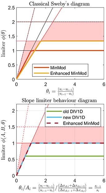
Where φ is the following enhanced MinMod slope limiter [47]:

For clarification, figure B1 compares behavior of normal slope limiters and enhanced slope limiters on differences and slopes for a non-equidistant grid. It is noted that numerical schemes with both normal and enhanced slope limiters are total variation diminishing (TVD) stable when applied to non-equidistant grids—e.g. in [7, 14]—as both satisfy the following sufficient condition [47, 48]:
The boundary cells lack a neighbor such that the standard slope limiter routine cannot be applied. For simplicity, we use the slopes to neighbors  . Alternatively one could use extrapolated quantities for cells mirrored behind the boundaries. Using the enhanced slope limiter φ, the advected quantities f are extrapolated to left (L) and right (R) boundary as follows:
Figure B1. (Top) Sweby diagram and (Bottom) adapted Sweby diagram to show a limiter acting on slopes instead of differences. Below the dashed lines given by equation (B.12) there is TVD stability and inside the red area the limiter scheme does not loose order in the solution moving from equidistant to non-equidistant grids. On display are the MinMod, enhanced MinMod for non-equidistant grid with  . The old and new DIV1D limiter schemes are displayed as function of slope next to the enhanced MinMod limiter.
Download figure:
Standard image High-resolution image
B.3.2. Flux limiter and Lax flux.
The flux limiter and Lax flux remain the same as in Dudson et al [14]. The advected fluxes on the cell boundaries  are calculated as:


where in addition to the slope limiter φ, a flux limiter  is applied in the form of:

which switches to a lower (superscript L) order upwind scheme for supersonic velocities, i.e.  . For subsonic flow, the higher (superscript H) order central scheme is used and a Lax flux is added to damp discontinuities allowed in the slope of the solution by the slope limiters. Note thus that there are two types of limiters, a slope limiter φi
different for each cell due to the non-equidistant grid and flux limiter
. For subsonic flow, the higher (superscript H) order central scheme is used and a Lax flux is added to damp discontinuities allowed in the slope of the solution by the slope limiters. Note thus that there are two types of limiters, a slope limiter φi
different for each cell due to the non-equidistant grid and flux limiter  switching between integration methods. Pressure gradients are discretized using a centered scheme for non-equidistant grids. For more details see [14, 47] and references therein.
In terms of equations this entails the following finite differences for the density, momentum, energy and neutral equations with i denoting the cell with cb, i and cb, i − 1, the upper and the lower cell boundary respectively:
At the boundaries the pressure gradients are calculated by forward or backward differences whereas the fluxes are determined by the boundary conditions.
B.4. Boundary conditions
At the target(s), the fluxes are calculated using the Bohm condition  with
with  , i.e.
  for isothermal flow toward the target. The target velocity and temperature are extrapolated from previous cell centers using equation (B.6). Accordingly, fluxes at the target(s) are:


The fluxes at the stagnation point are set to zero for a zero gradient boundary for the solved quantities.
B.5. Numerical viscosity
In the implementation discussed so far there are two issues to be noted. Firstly, the Bohm criterion  is not always satisfied because the velocity in the last cell in front of the target drops for an unknown reason. Secondly, for high resolution grids, numerical oscillations appear. To combat these issues, a numerical viscosity is implemented to penalize second order derivatives in the velocity profile and deviations from the Bohm criterion.