
Abstract
In this work, a very fast integrated transport model involving every region that interacts directly with the plasma of a tokamak, has been developed. The confined region is modeled in 1.5D, while the scrape-off layer has a 0D structure. For the core region, a physics-based analytical regression based on a set of simulations with the transport model TGLF [Staebler 2005 Phys. Plasmas 12 102508] has been produced. For the H-mode regime, an average edge-localized-modes model is applied in the pedestal region. In the scrape-off layer a two-point model for electron temperature (exhaust) and a particle balance for the species density at the separatrix have been implemented. All the models have first been validated individually in a standalone setting. Finally, six fully integrated simulations of an L-mode discharge, and five H-mode discharges, have been performed in the Fenix flight simulator [Janky et al 2019 Fusion Eng. Des. 146 1926, Fable et al 2022 Plasma Phys. Control. Fusion 64 044002], including transients, matching the experimental trajectories of an ASDEX upgrade discharge during flat-top and ramp-down. A broader validation including more discharges and the ramp-up phase is planned for the near future.
Export citation and abstract BibTeX RIS

Original content from this work may be used under the terms of the Creative Commons Attribution 4.0 license. Any further distribution of this work must maintain attribution to the author(s) and the title of the work, journal citation and DOI.
1. Introduction
The ability to predict the evolution of a new plasma discharge can allow one to improve the efficiency of the discharge itself. Moreover, it has become increasingly clear that a fast and reliable predictive ability for the entire evolution of a planned tokamak discharge is required for the operation of reactors like ITER and DEMO, before the plasma discharge is actually performed. This prevents undesired events, like disruptive cases, from occurring in actual experiments, avoiding major damage and the interruption of the reactor operation, with consequent costs of reparations and long delays. Several ways to perform these predictions already exist, and they differ in the level of detail and required computational time. The easiest formulae available are the scaling laws [2, 3], which predict the confinement time of a stationary phase of a discharge. However, they cannot be used to predict the plasma evolution of an entire discharge, including transients. Moreover, they are 0D and miss a physics-based nature, so their applicability and reliability is reduced. In fact, they miss the profile effects, which can be very important for the discharge evolution and to predict certain conditions, like internal transport barriers (ITBs). The predictions can be also made by adopting different suites or codes. For this purpose, more complex models like gyrokinetic or fluid codes can deeply describe the physics, but they are time-consuming. Furthermore, during experimental campaigns some 'last-minute' changes in the discharge program could be applied due to technical reasons, just before running the discharge. Therefore, the need for fast simulations based on first principles has become clear. A predictive tool that meets these prerogatives is the tokamak flight simulator, Fenix [4, 5]. This is a numerical tool that predicts the plasma behavior using the discharge program as input. It is based on the interaction between a control system, which is simulated within Simulink, and a physics model, which mainly includes equilibrium and transport models. It can ensure that either actuator trajectories or plasma parameters satisfy the experimental goals and reduce the probability of plasma disruptions and of exceeding operational limits. While the plasma equilibrium and the control algorithm can already be described analytically, a fully integrated analytical transport model is still missing. This has to be physics-based to be realistic, but also fast enough to be used as an inter-discharge prediction tool. This compromise can be reached by employing analytical models that are derived from first principles theories. An important task in the development of these models is to include as few experimental inputs as possible to strengthen the prediction capability. As a starting point, Fenix was initially tested with models in which the transport was tuned to match some experimental measurements.
An alternative solution based on first principles, which strongly reduces the amount of experimental input, is proposed in this work using a set of four transport physics-based models. Two models are applied in the confined region, depending on the regime of the plasma, while the other two act in the scrape-off layer (SOL). They are linked through the last closed flux surface (LCFS). At this point, the models of the SOL give boundary conditions for the confined region, taking as input engineering parameters, which can be scheduled during the discharge's plan. Moreover, these fast analytical models can be implemented in the flight simulator, so that it can be used inter-discharge to predict the discharge evolution. When coupled with a predictive model for the disruptions, Fenix could also allow the avoidance of disruptive cases. Such a model still does not exist, but its development has been planned for future work. A possible simple approach could be to couple Fenix with a space state description that sets the conditions for which the plasma hits some hard limits (e.g. high density limit, as in [6]).
The models have been developed in the framework of the transport code ASTRA [7, 8]. This framework allows us to couple the different parts of the tokamak simultaneously, giving boundary conditions to each other. Although ASTRA, like any other transport code for confined plasma, does not contain any radial grid beyond the LCFS, additional subroutines are flexibly coupled, which (virtually) simulate the evolution of the SOL concomitantly with the evolution of the confined plasma. The analytical nature of all the models allows for an iteration-free working principle in which all the models proceed concomitantly, interacting with one another through their boundaries.
In section 2 the core model is shown, in section 3 the edge model is presented, while in section 4 models for the SOL are explained. Section 5 shows six first fully-integrated simulations for five H-mode discharges and an L-mode AUG discharge in the Fenix flight simulator. Conclusions are drawn and the outlook described in section 6.
2. Core model
The core of a tokamak plasma is defined here as the region up to  , where ρt
is the toroidal magnetic flux minor radius normalized to the value at the separatrix. This definition of the core comes from the choice of the pedestal width. In fact, this has been fixed equal to 0.1 in ρt
units. Moreover, almost all the simulations run to build up the core transport model were performed along the radius up to
, where ρt
is the toroidal magnetic flux minor radius normalized to the value at the separatrix. This definition of the core comes from the choice of the pedestal width. In fact, this has been fixed equal to 0.1 in ρt
units. Moreover, almost all the simulations run to build up the core transport model were performed along the radius up to  , which is the region where the code used to perform such simulations has already been widely validated in earlier works.
The plasma reaches its highest values of pressure in the core. In this region, when the kinetic pressure is high enough, the fusion reactions can happen. Nevertheless, some dynamics are found to be opposed to the increase of plasma energy, and in some cases they can set a constraint on the maximum reachable pressure and energy. The main phenomena involved in this are the magnetohydrodynamic (MHD) instabilities and the heat and particle transport. The last two are in turn split into neoclassical and anomalous parts. This work focuses on the anomalous (turbulent) transport. Some fast models already exist and they are based on neural networks (NNs), like Qualikiz NN [9]. However, NNs need training on a wide database which can assure that the model will work properly inside the range of variation of the data collected, but it could be unsuccessful outside it, so its use could be compromised. This is particularly important when one extrapolates to larger devices, which is a crucial problem for machines of the next generation. Moreover, even if the NNs can provide a correct prediction of transport coefficients, their structure does not offer physics insights. For all these reasons an alternative model, based on analytical formulae fitted over a smaller database than the one usually needed from a NN, is proposed here. Its theoretical nature, which is based on first principles, offers more transparency and physics insight, as well as an easier extrapolation to larger or different devices. In fact, the coefficients derived in this work are multiplied by a gyroBohm scaling factor which takes into account the dependence on  , which is the main parameter to take into account in the extrapolation to bigger machines. In order to define the formulae of the transport coefficients, the main instabilities affecting the core have to be considered. In this region they are the micro-instabilities driven by temperature and density gradients. It has been shown by experiments that this transport has a threshold nature [10, 11]. It is also known that there are some stabilizing effects on these instabilities (e.g. collisionality, magnetic shear, impurity concentration, β, concentration of fast particles and E × B shear) [12–17] and that shape plays a role [18]. Therefore, taking into account all these aspects, some threshold formulae have been adopted for ion temperature gradient (ITG), electron temperature gradient (ETG) and trapped electron mode (TEM) and fitted to a database of TGLF [19–21] simulations, while micro-tearing modes (MTMs) [22–24] have been neglected, because they are usually negligible with respect to the ITG/TEM transport in the core region. This is anyway not always true, especially in spherical tokamaks [25] or in some configurations with high β, which is the main drive of MTM, or in some ITG suppressed advance scenarios. However the database used in the fitting does not include such discharges, but the development of a formula to take into account this instability in an extended database of discharges is planned for the future. TGLF simulations were set in this way: saturation rule 2 (which sets a specific rule for the fitting of the quasilinear fluxes of TGLF on some nonlinear gyrokinetic simulations), three species (electron, D and B/N) and electromagnetic effects. The database consists of some stationary phases of 15 AUG discharges from different scenarios (H-mode, L-mode, I-mode and negative triangularity). Each of these cases has been perturbed in the boundary condition of the kinetic profiles by enhancing/reducing by 10% electron density, electron temperature and ion temperature at
  . This scan has increased the database and assured that the range of variation of the normalized gradient of the kinetic profiles is covered in a more homogeneous way, with a contiguous spread of the data. This should improve the quality of the fitting. The broad variety of configurations included in the database is largely justified by the general nature of the instabilities treated. In this database, six coordinates in the range
 ![$\rho_t = [0-0.9]$](https://content.cld.iop.org/journals/0741-3335/65/3/035007/revision2/ppcfacb2c6ieqn5.gif) have been considered for the last 20 time steps of the converged TGLF+ASTRA simulations. The simulations included sawteeth, but a strategy to exclude their impact on transport has been used, based on varying the position of the first radial coordinate included in the fitting. Moreover, some coordinates at
have been considered for the last 20 time steps of the converged TGLF+ASTRA simulations. The simulations included sawteeth, but a strategy to exclude their impact on transport has been used, based on varying the position of the first radial coordinate included in the fitting. Moreover, some coordinates at  for one L-mode case are included. Thus, it is possible to use this model in the edge in the L-mode configuration, where turbulent transport is still determining the profiles. The database consists overall of 12 600 values of
  and
and  , which are respectively electron and ion heat diffusivity. The database is much smaller than the one usually needed in a NN model, but considering that the maximum number of fitting parameters involved is 15, there are almost 1000 data for each free fitting parameter, and so we have confidence that there are enough data to catch all the dependencies of the formulae and to give a reliable result. The formulae used for the fitting are reported here, in gyroBohm units [26], that is
  , where r is the minor radius:


where R is the major radius,  , q is the safety factor, βe
is the ratio between electronic kinetic and magnetic pressure, k is the local elongation, δ is the local triangularity,
, q is the safety factor, βe
is the ratio between electronic kinetic and magnetic pressure, k is the local elongation, δ is the local triangularity,  is the main ion fraction, ν is the collisionality, defined as
  with ne
in
with ne
in  , Te
in keV and
, Te
in keV and  equal to effective charge, s is the magnetic shear and ft
, defined as
equal to effective charge, s is the magnetic shear and ft
, defined as  , is analogous of the trapped particle fraction, while C,
  10, γq
,
10, γq
,  , γk
,
, γk
,  , D, 20,
  ,
,  , D2, 30, γν
, γs
,
, D2, 30, γν
, γs
,  , D3 are the fitting parameters. H is a Heaviside function, whose argument is the difference between the normalized temperature gradient and its threshold value. 10, 20 and 30 are the exponents of the differences between the actual normalized gradient and its threshold, representing thus the stiffness, which determines how the kinetic profiles react to the enhanced heating. The electromagnetic effects due to the fluctuations of magnetic fields are included through the β term, as a combination of magnetic flutter and stabilization of ITG modes, resulting in an overall reduction of transport. The shape of the plasma also affects the transport, because it changes the relative length that the particles travel in the high field side (HFS) and in the low field side (LFS), affecting thus the ballooning stability. The shape also changes the local concentration of particles, creating an additive poloidal redistribution. In order to take into account these effects, δ and k are included in the formulae. The collisionality is a crucial parameter to distinguish between different instability regimes. In particular, it reduces the effect of the trapped particle fraction, through collisions with passing electrons. This is modeled in
  , through
  . The magnetic shear reduces the transport, through the tilt of the field lines, which leads to a decorrelation of the neighboring field lines. This effect is taken into account through the terms related to q and s in the formulae. For
  a proportionality with
  has been assumed, through the trapped particle fraction (because the passing electrons are considered adiabatic for this instability) and a ratio between electron and ITG (to simulate the relative contribution of electrons to a ionic instability). The linear threshold formulae are available from the literature [27, 28]. For the ETG and ITG thresholds, some fitting parameters have been added to multiply some dependencies:
where  , while A10, B10, B20, A20, F10, G10, G20, F20 are other fitting parameters. The ITG threshold has the same shape as the ETG one, except
  is inverted, because in the linear limit the two instabilities have the same physical picture [29]. In the threshold formulae the dependence on
  appears to take into account the contribution of the ions and the electrons, respectively, to the electronic and ionic instabilities.
Starting from the outputs of the ASTRA simulations, some TGLF standalone simulations have been run for each radial coordinate of each discharge. It has been found that the contribution of transport due to  instabilities is a very small percentage of the total transport. Considering that this is the only spectral region where ETG appears, the need for another database becomes clear, one that is more focused on the ETG-wavelength instability region. This has been obtained by multiplying the original database of
  in output from ASTRA by
  , where
  is the anomalous electron heat coming from
  transport, and
  is the total transport over all the spectra. This ratio represents the percentage of electron heat transport due to small scale turbulence. Considering that the temperature gradient is constant over the spectra
  , because
  is assumed to be due to ETG. This should provide a rough distinction between ion scales and mixed-electron scales. This procedure has led to a disentanglement of the microinstabilities, which are fitted separately, leading to a reduction in degrees of freedom, which goes more in the direction of a physics-based fitting rather than an artificial fitting, whose success is a coincidence of numerical optimizations. However, one could in principle contest the rough separation between ETG and TEM+ITG contributions made by splitting spectra in two clear regions. To overcome this problem, a first fitting on the ETG database has been performed by also including
  formula, and it has been seen to match a branch of high
  values. In fact, a clear difference between the
  matched by the ITG formula and by the ETG formula has been found in terms of parameter dependencies and order of magnitude. A filter to separate these two branches of coefficients has been put in place by excluding data with both
  and
and  (in gB units) conditions met. Those conditions have been found to belong to ITG-driven cases. Anyway, an unavoidable small residual contribution from TEMs is present in the ITG-filtered database, due to the fact that this instability appears also on electron scales. The ETG threshold has been fitted, because in this way it was found to better match the TGLF output. The results show stronger
  and lower s and
  contributions in the linear ETG threshold with respect to the formula from the literature. This effect could be due to a residual presence of
  -driven TEM, which is not included in the model. In fact, a threshold formula is present in the literature, but the hypothesis under which it is valid is too constraining (no temperature fluctuations). Another cause of it could be the difference between the linear and nonlinear ETG threshold, where the second is found to produce stronger transport due to the formation of ETG streamers [29–32]. However, TGLF is a quasilinear model; then, the presence of a nonlinear threshold could be just the result of the multiscale spectral calibration over the gyrokinetic database fitted to obtain the saturation rule (i.e. is not a theoretical threshold but the result of a fitting procedure). An additional formulation of the density gradient drive of TEM is planned for the future. The TEM threshold has been chosen not to contain fitting parameters in order to reduce the degrees of freedom during the fitting process and optimize the iteration procedure. One can see that the main stabilizing effects have been taken into account, in the threshold or in the coefficient expressions, while the stiffness is assured by the power law on the difference between normalized gradients and their critical values. Also, cross dependencies, which are effects of a species-related instability on other species, have been included by
  . This means that ITG in this model also drives some electronic heat transportin particular, due to the trapped electron contribution in the ITG mode.
Figures 1 and 2 show the scattering of the fitted coefficients compared to the respective values calculated by TGLF. The red points are the values calculated using the fitting formulae, while the respective TGLF values lay on the black solid line. The coefficients are shown in gyroBohm units. One can see that the general trend is reproduced, and some scattering should be tolerated considering that the coefficients are taken along the entire radius (up to separatrix in few cases) and the simple structure of the analytical formulae. Anyway, some analytical coefficients are completely mismatching the values from TGLF, which is the case of the spot of red points around  . These cases were investigated to understand the nature of the mismatch and the safety factor was found to be below 1, so it is argued that the sawteeth model has increased the TGLF coefficients. The means and the standard deviations of the ratios between the fitted and the TGLF transport coefficients for
  ,
,  and
and  are, respectively,
  ,
,  ,
,  ,
,  ,
,  ,
,  .
.

Figure 1. Transport coefficients derived by the fitting formulae vs those calculated by TGLF. The red points are the values calculated by the analytical formulae, while the solid line represents the respective values computed from TGLF. On the left is shown ion heat diffusivity, while on the right TEM+ITG electron heat diffusivity. The coefficients are shown in logarithmic scale.
Download figure:
Standard image High-resolution image
Figure 2. Transport coefficients calculated with the ETG fitting model vs those computed by TGLF for  . The red points are the values calculated by the analytical formulae, while the solid line represents the respective values computed from TGLF. The coefficients are shown in logarithmic scale.
Download figure:
Standard image High-resolution imageFigures 3–5 assure the wide range of variations of most of the parameters and show that most of the parameter dependencies are well captured, proving the successful performance of the fitting routine. However, in figure 3(c) a branch of analytical χi
could not match the TGLF values. In fact, in this plot, one can clearly see a bifurcation of the dependence of χi
on  , where one branch is increasingly weaker and the other is very steep. In order to investigate the mismatching χi
with strong
, where one branch is increasingly weaker and the other is very steep. In order to investigate the mismatching χi
with strong  dependence, the input parameters of two simulations with
  giving, respectively,
  and
and  , were selected, and some scans around the nominal input parameters were performed with TGLF stand alone. After a detailed analysis, the main reasons for the difference between the transport coefficients in the two cases were identified for different values of collisionality and radial position (and trapped particle fraction). In particular, the collisionality of the high χi
case was three times the one of the low χi
, while the normalized minor radius of the former was 1.5 times the one of the latter. This is not surprising because high collisionality usually drives transport by shifting upwards the saturation level given by zonal flows [33]. Anyway, the similar values of the other parameters (in particular the high value of magnetic shear) should prevent the triggering of an ITG for both the cases, while the TEM should be reduced by high collisionality. The differences between the two χi
have been compared to two corresponding linear calculations with the gyrokinetic code GENE, using the same input parameters as the TGLF cases. In the high collisionality case, the growth rate spectrum of GENE is found to be one order of magnitude smaller. Correspondingly, also a quasi-linear estimate of the ion heat flux using the GENE results and applying a quasi-linear rule, which is analogous to that of TGLF ,yields values which are one order of magnitude lower than the TGLF. This comparison with GENE, and the observation that the TGLF predicted ion temperature profiles in these conditions are significantly below the experimental ones, consistent with a TGLF overestimation of the heat conductivities in comparison to the power balance ion heat conductivities, suggested neglecting this branch of TGLF results in the derivation of the analytical model. Anyway, a further investigation with nonlinear gyrokinetic simulation is well beyond the scope of this work. It is worth noticing that the branch of mismatching χi
in figure 3(c) is reflected also on χe
in figure 4(c), through the term
, were selected, and some scans around the nominal input parameters were performed with TGLF stand alone. After a detailed analysis, the main reasons for the difference between the transport coefficients in the two cases were identified for different values of collisionality and radial position (and trapped particle fraction). In particular, the collisionality of the high χi
case was three times the one of the low χi
, while the normalized minor radius of the former was 1.5 times the one of the latter. This is not surprising because high collisionality usually drives transport by shifting upwards the saturation level given by zonal flows [33]. Anyway, the similar values of the other parameters (in particular the high value of magnetic shear) should prevent the triggering of an ITG for both the cases, while the TEM should be reduced by high collisionality. The differences between the two χi
have been compared to two corresponding linear calculations with the gyrokinetic code GENE, using the same input parameters as the TGLF cases. In the high collisionality case, the growth rate spectrum of GENE is found to be one order of magnitude smaller. Correspondingly, also a quasi-linear estimate of the ion heat flux using the GENE results and applying a quasi-linear rule, which is analogous to that of TGLF ,yields values which are one order of magnitude lower than the TGLF. This comparison with GENE, and the observation that the TGLF predicted ion temperature profiles in these conditions are significantly below the experimental ones, consistent with a TGLF overestimation of the heat conductivities in comparison to the power balance ion heat conductivities, suggested neglecting this branch of TGLF results in the derivation of the analytical model. Anyway, a further investigation with nonlinear gyrokinetic simulation is well beyond the scope of this work. It is worth noticing that the branch of mismatching χi
in figure 3(c) is reflected also on χe
in figure 4(c), through the term  in equation (4).

Figure 3. Dependency of χi on the physical parameters included in the fitting. In blue, the values from the TGLF database, in red the ones respectively calculated by the fitting model.
Download figure:
Standard image High-resolution image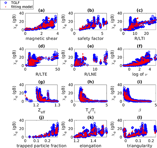
Figure 4. Dependency of  on the physical parameters included in the fitting. In blue the values from TGLF database, in red the ones respectively calculated by the fitting model.
Download figure:
Standard image High-resolution image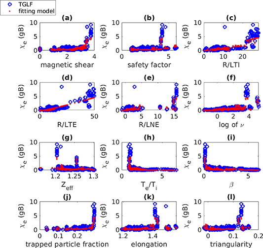
Figure 5. Dependency of  on the physical parameters included in the fitting. In blue the values from the TGLF database, in red the ones respectively calculated by the fitting model.
Download figure:
Standard image High-resolution imageIn figure 5 each of the 12 plots shows a subset of TGLF χe
which are not matched by the ETG analytical formula. This is probably caused by a minimum residual of ITG-driven transport in the TGLF database used for the ETG fitting. This is supported by the fact that the trend in  is captured except for high values of the normalized gradient, which is consistent with the presence of ITG. Moreover, the mismatching transport coefficients are underestimated for low values of β, which reduces ITG. Some other mismatching χe
could be due to the presence of TEM-driven TGLF transport coefficients, because most of these χe
mismatch for high values of trapped particle fraction and high values of density gradient, which can drive TEM. The presence of residual TEM transport is also supported by the larger heat conductivities for high
is captured except for high values of the normalized gradient, which is consistent with the presence of ITG. Moreover, the mismatching transport coefficients are underestimated for low values of β, which reduces ITG. Some other mismatching χe
could be due to the presence of TEM-driven TGLF transport coefficients, because most of these χe
mismatch for high values of trapped particle fraction and high values of density gradient, which can drive TEM. The presence of residual TEM transport is also supported by the larger heat conductivities for high  . Anyway, the ETG contribution to the transport was found to be smaller than 5% for most cases, so its relevance is reduced in this work. A better formulation of the ETG transport is planned for the future.
The means and standard deviations of  for different values of the parameters included in the fitting are shown in figures 6–8 respectively for
  ,
,  and
and  . Here, one can see the most critical values of the parameters in which the standard deviation is high, then where the fitting procedure loses quality and does not match the TGLF values.

Figure 6. Mean and standard deviation of  depending on the different physical parameters included in the fitting.
Download figure:
Standard image High-resolution image
Figure 7. Mean and standard deviation of  depending on the different physical parameters included in the fitting.
Download figure:
Standard image High-resolution image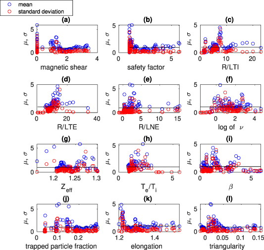
Figure 8. Mean and standard deviation of  depending on the different physical parameters included in the fitting.
Download figure:
Standard image High-resolution imageThe output fitting parameters are:
The particle diffusivity has been assumed to be equal to  , where C is a calibration factor which has been fixed equal to 1 to match the kinetic profiles of a discharge, while particle pinch has been modeled with a heuristic formula which is proportional to diffusivity to assure stationarity and takes into account the effect of
  , s and ν [34–38]
The maximum function has been used here to assume a negative convection, that is a pinch, in order to have stationarity through the balance between particle diffusivity and particle pinch. This is not a really strong assumption for AUG discharges. A physics-based model for particle transport is a task that has not yet been performed, due to the difficulty of modeling the particle convection, whose value can change sign locally. However, an improvement of the model used here is planned for the future. The database shown has been built using TGLF with saturation rule 2, but earlier saturation rule 1 has also been adopted, in order to strengthen the fidelity of the procedure used in the model. Also, in this case , a small scattering of the TGLF coefficients around the fitting values has been found, but the main dependencies are well reproduced by the formulae.
3. Edge model
The model described in the previous section is, in principle, extendable to the entire confined region. However, this is not always possible due to the different physics which govern the edge of the plasma in some specific configurations. In fact, in the high-confinement regime (H-mode) or the improved confinement regime (I-mode), which are observed when a threshold in heating power is overcome, a pedestal arises respectively in both density and temperature, or only in temperature profiles. This pedestal is formed in a small region of the plasma near the LCFS, or separatrix, but it plays an important role, because it sustains a sizeable fraction of the plasma energy. In this region, steep gradients in the kinetic profiles can be sources of free energy and the presence of the bootstrap current, which modifies the current profile and the safety factor, can affect the turbulence. Moreover, a combination of destabilizing and stabilizing effects, for instance connected with the strong gradients, the high safety factor, the collisionality and the plasma beta, as well as magnetic and rotational shear, imply that the pedestal can host a variety of instabilities and consequent turbulence featuring different thresholds and transport properties. Therefore, a quantitative prediction of the transport in these conditions is not a trivial task. Nevertheless, a simplified approach can be used in the flight simulator, since it will give the boundary condition for the core model even if the pedestal structure is not captured in detail. To distinguish this region from the core another model has been used starting from  , which is assumed to be the position of the top of pedestal, outwards. The pedestal width is then assumed. This assumption comes from the absence of a pedestal transport model, that coupled with an MHD stability model could calculate consistently the pedestal width. The choice of
  as top of pedestal position has been made to bound smoothly core and edge models. Some tests have been done changing this position up to
  and no big impact has been found on the results. Some pedestal transport models to estimate the pedestal width exist (e.g. EPED [39] and IMEP [40]) but it was hard to implement them in a fast flight simulator, because they need to compute MHD stability. A self-consistent calculation of the pedestal width is anyway planned as future work, because its prediction can be crucial for MHD stability in some ELM-free or reactor-relevant scenarios. It is known that in high-confinement mode (H-mode) the dynamic is usually mainly dominated by edge localized modes (ELMs) [41, 42], which are MHD instabilities, while micro-instabilities are often reduced by sheared flows (as ExB shear) [43], even though some residual turbulent transport is still present, as was discussed previously. In this configuration, an ELM average model has been adopted and the diffusivities have been assumed to lay on the marginal stability limit of the MHD peeling–ballooning model [44, 45]. This approach is justified by the fact that it is behind the goal of this project to accurately reproduce the temporal evolution of the instability, as could be done by a high fidelity code or any discrete ELMs model. Furthermore, the temporal scale of these instabilities is much shorter than the duration of the discharge or the reaction time of the control system, so one can assume an average behaviour without leading to big limitations of the model when it is used within a flight simulator. Any discrete ELMs model could be added in the future. By assuming a marginal stability on the MHD peeling–ballooning boundary, a heuristic formula has been derived, which is based on a power law of the ratio between
  at the top of pedestal and
  , which is the critical value for the onset of the instability
The critical value of βp is

which is a scaling that has been obtained from an EPED [39] database, according to [46]. Here,  is the electron density normalized to the Greenwald limit, while wp
is the pedestal width in the normalized poloidal flux label, which is fixed to 0.1. This is a good assumption for AUG, but it needs to be generalized in order to extrapolate to other devices. This scaling also includes the effect of the shape, which allows us to take into account and also predict the purely peeling or peeling-ballooning limited cases.
is the electron density normalized to the Greenwald limit, while wp
is the pedestal width in the normalized poloidal flux label, which is fixed to 0.1. This is a good assumption for AUG, but it needs to be generalized in order to extrapolate to other devices. This scaling also includes the effect of the shape, which allows us to take into account and also predict the purely peeling or peeling-ballooning limited cases.
 has been assumed in this case, supported by [40]. The particle diffusivity has been fixed to be equal to
  , where C has been fixed to 0.03 to match experimental stationary profiles in some discharges. This is still in agreement with [40].
In the low-confinement regime (or L-mode, i.e. when the power threshold is not overcome), the fitting model used for the core has simply been extended to this region, while particle diffusivity is kept equal to  , where F is calibrated to match experiments in the database (F = 0.1).
In order to predict the transition between L- and H-mode, criteria based on the ion power crossing the separatrix has been chosen, according to the Schmidtmayr scaling [47]. This scaling has been previously tested successfully on different H-mode discharges. Differences in pedestal widths between density and temperature [48, 49] have been neglected.
The simulation of ELM-free scenarios (e.g. I-mode, EDA H-mode or negative triangularity) can be more challenging, due to the complicated and wide physics involved in the edge. These scenarios are very attractive for future reactors, therefore at least some reduced prediction capability should be included. Then, for these configurations some ad-hoc models are present, which have a less physics-based nature, due to the fact that the dynamic involved is still not fully understood. For the transition from L- to I-mode a scaling derived in [50] has been used. During the transition, a pedestal arises only for the temperatures, while the density remains equal. For the negative triangularity discharges, a correction on the L–H transition has been numerically introduced to modify the power threshold.
4. SOL models
A model of the SOL needs to be included to create a fully integrated model. Its role is to furnish boundary conditions at the separatrix for the confined region. An important task is to reduce the amount of experimental input to strengthen the prediction capability. However, a minimum number of experimental fit parameters, which are often machine-related, is necessary due to the more complex physics and the weaker theoretical description of this region. Moreover, the dynamic in the SOL depends on the systems facing the SOL and some parameters can be machine-dependent. Two different models have been implemented to provide electron density and temperature at the separatrix.
4.1. Power exhaust
Several aspects should be taken into account concerning the power exhaust modeling, because this indirectly influences the fusion performances and fixes some technological constraints for large-size future machines. The two-point model has been largely validated across the years [51–56]. Its 0D structure based on a power balance between the outer midplane (OMP) and the divertor target makes it adequate for use in our work. Obviously, its implementation leads to a lack of detail about directional phenomena, radiation and more complicated aspects, but still represents a good candidate to obtain the necessary elements for a fully integrated code, thanks to its physics-based nature.
A simple formula to determine the electron temperature at the separatrix has been derived in [54], which can be used in the attached condition:
Here,  is the parallel electron heat flux,
  is a dimensionless factor used to account for extended field-line lengths in alternative configurations, k0 is the parallel electronic conductivity for Z = 1 divided by
  ,
,  is a safety factor defined as in [54], R is the major radius, and
  .
.  is assumed equal to
  .
.
The main limit of this model is that it does not include a consistent radiation model and it is derived for the attached condition, i.e. without pressure losses along the magnetic field lines. However, detachment modeling has to be included in the future because it is a necessary condition that has to be reached by machines of the next generation in order to prevent exceeding maximum heating loads and damage to the plasma facing components (PFCs). The modularity of the integrated model allows the future updating of the formula under detachment conditions. The formula shown needs  at the separatrix, which is not provided by the model for the confined region. This 'external' parameter is provided by the particle balance model in the SOL, which gives the value of the density at the separatrix for all the ion species. This model is discussed in the next section.
4.2. Particle balance
The proper treatment of particle diffusion in the SOL is a complicated task that can be pursued by the use of time-consuming codes, which include neutral treatment, such as SOLPS-ITER [57, 58]. This is beyond the scope of this work. Nevertheless, a simplified model can be used to translate engineering parameters into boundary conditions for the separatrix. Some formulas have already been used in the past for AUG, for example, in [59]. However, these are often related to the technological aspects of a specific experiment, so they miss general validity. Moreover, they are not time-dependent, which makes them inadequate for use in a flight simulator. This is the reason why a model that takes into account the minimum possible amount of experimental observations and more detailed geometrical aspects, has to be developed. This can be done by using a multispecies 0D particle balance that takes into account only the main features related to different regions included in the SOL, but ignores any directional detailed dynamic. For this purpose, in the model developed, the SOL has been split into six different zones that communicate with each other. These are the two divertor legs, the PF, the two upper sides of the tokamak cross section, and an additional zone close to the wall on the LFS. The splitting of the SOL region into the different zones is shown in figure 9. Such splitting can possibly be modified according to different divertor configurations by manipulating the regions (e.g. including another upper private flux region (PFR) in the case of a double null configuration, i.e. DN). Every region has different aspects to be taken into account, even though the main physics is the same. This allows a modular treatment of every zone, without losing the generality of the background structure. The model consists of a particle balance between all the confining regions, which includes diffusive terms, ionization sources, recombination sinks and sources of plasma coming from LCFS. The recombination sinks are assumed to be equal to zero, which is consistent with the assumption of the attached divertor. Gas puff and vacuum pump are also included as source and sink in the regions where they work. These are examples of the possibility of treating local effects in the respective zones. One other example is the recycling factor, which is only modeled in the wall zone (i.e. low recycling regime), even though a more precise description of it, including both the divertor legs, is planned for the future. This parameter is equal to 0.99 for D and H. Moreover, a diffusivity between this last region and outside the tokamak has been assumed (leakage), while for all the other zones, perfect reflectivity of the PFCs has been considered. Some coefficients have been added to the equations to keep concentration gradients between confining regions unbalanced, in order to mimic convection. These are called enrichment factors and they multiply the density of species:
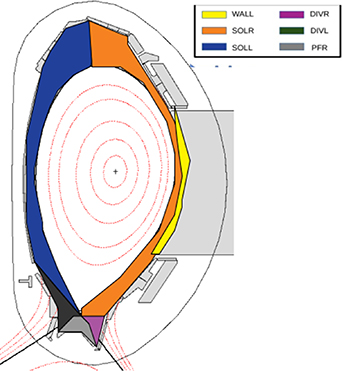
Figure 9. Splitting of the SOL region into six different zones.
Download figure:
Standard image High-resolution imageIn the previous equation Sk
represents the source term, which also contains the plasma coming from the confined region through the separatrix, Pk
is the sink, Djk
is a 0D diffusion coefficient defined as an exchange rate between the regions j and k (in m s−3), N is the number of particles, V is the volume and jk
is the enrichment factor. From these balance equations, the temporal evolution of particle density in every region can be found. The average between the densities of the two upper parts of the SOL (SOLL and SOLR) is assumed to be equal to density at the separatrix, according to the 1.5D structure of ASTRA. In the model, a multispecies treatment is included up to eight species, but this number is arbitrary because it does not greatly impact the computational time, due to the analytical nature of the equations. One can possibly build neutral modeling in a similar way, by considering recombinations as sources and ionizations as sinks. This model is necessary to simulate detachment conditions. Considering six equations like (15) for six regions, the following system can be derived for each species:

where  is the vector of the particle number for every region, j index indicates a specific species,
  is the vector that includes all the local effects (ionizations, recombinations, recycling, vacuum pump or gas puff) and
  is the matrix of the diffusivities normalized by some factors, which also include the enrichment factors. The system is calculated implicitly.
This model allows us to calculate the density at the separatrix with gas puff and vacuum pump velocity as inputs, reducing so the necessary experimental data to the engineering parameters, which are controllable and needed anyway for the discharge plan. However, a crucial problem is the determination of the diffusivities between confining zones. These have been derived heuristically, considering the main contributions to the parallel and perpendicular particle transport:
Here, the 'sep' subscript stands for separatrix, M is the sound velocity, calculated as  , where
  is the deuterium density,
  is an estimate of the distance traveled by the particles along the field lines and it is calculated as
  , Rw
and
, Rw
and  are the major radius at the wall and OMP positions.
  ,
,  and
and  were calculated assuming convection as the dominating parallel transport.
  and
and  were fixed to 0.1 to mimic a lower transport between the divertor legs across the PFR with respect to the parallel transport along the field lines, which is a reasonable assumption for ions [60] in L-mode. The high gradients between divertor legs and PFR ensures a higher value of diffusion across the PFR in H-mode [60].
  has been fixed to 0 to neglect the transport from the wall directly to the divertor (i.e. perpendicular transport is the only dynamic assumed in the thin layer of plasma near the wall).
  and
and  , which represent the perpendicular transport in the LFS, have been assumed proportional to the collisionality, according to [61], neglecting poloidal asymmetries. In particular,
  has been multiplied by 0.5 which is the standard value used in SOLPS calculations [62, 63], while
  has been multiplied by 0.03 to take into account a certain level of D wall retention, which counteracts the outwards diffusion. The previous equations contain some numerical factors which represent the calibration of the model to match an experimental case.
These coefficients do not take into account the drifts, which have been modeled by employing some enrichment factors, that keep the densities of confining regions unbalanced and ensure a certain background level of diffusion. In this way, the compression factors can be taken into account. The enrichment factors are
in favourable configuration (i.e.  ), while in unfavorable configuration
  . This last coefficient has been used to model a
  drift correction, which is assumed to be inversely proportional to the size of the machine and includes an aspect ratio dependence. 34 has been fixed to 10 to modulate a certain background level of HFS high density front [62, 64, 65]. 26 is a derivation of the steady-state formula of [59], which has also been successfully implemented in IMEP [40], for a time-dependent situation.
  is the density of D or H at the divertor. Also, here the numerical factors are calibrated to match the separatrix electron density of an H-mode AUG discharge in the flight simulator. A better formulation of the enrichment factors including detachment, X-point radiator [66],
  and E × B drifts is planned for the future. All the particle diffusivities and enrichment factors shown here are used for D or H, but similar formulae are also applied for impurities, taking into account some technological aspects, like W sputtering, B coming from the boronization of the machine and N seeding. In particular, the W sputtering is roughly modeled by adding a simple constant input of this species in the SOL. A similar approach is used for the residual B coming from the boronization.
The temporal evolution of D ions in a Fenix simulation of the H-mode #40446 discharge is shown in figure 10, together with the D gas puff. In this figure, one can see that the densities above the X-point are one order of magnitude lower than the regions below. This is consistent with many experimental observations and theoretical predictions, especially if the source coming from the divertor region (e.g. by ionizations) is bigger than the one from the OMP. One can also notice that the PFR density is lower than those of the divertors for  , while it lays between the inner and outer divertor values for
  . These two temporal ranges are before and after the onset of H-mode, and it is consistent with observations from [60]. It is worth mentioning that the only parameters that depend on the temperature are the ionization coefficients of H, D and He. It is still complicated to run simulations with both power exhaust and particle balance models because they depend on each other's output.

Figure 10. Left: D OMP gas puff evolution for discharge #40446. Right: temporal evolution of number of D ions in the SOL for the discharge #40446. Different colors show the densities in the different regions, as shown in figure 9.
Download figure:
Standard image High-resolution imageThe main limit of the model is the presence of a specific divertor configuration, which is lower single null (LSN). As already mentioned, other configurations (e.g. upper single null, i.e. USN, and DN) can still be included by splitting the SOL into more zones, while maintaining a similar approach in describing the particle content in each zone. Anyway, the model has been validated only against LSN configurations, thus further validation with other configurations is needed. Another limitation is the modeling of the X-point radiator and detachment, which are still not included, but they could be implemented by adding the treatment of neutrals in the particle balance and modifying the enrichment factors, without changing the background structure. Finally, there is no description of transport and heat and particle loads deriving from ELMs. This is really important to prevent any damage to the divertor, but should not have much affect on the evolution of the global parameters, which are of primary importance in a flight simulator. Moreover, the W influx should be independent of the conditions of the divertor, even in the presence of ELMs, because the region which rules such quantity in AUG is the main chamber [67]. Then the same model with the same tuning coefficients is used for both L- and H-mode. We are aware that such limitations reduce strongly the physical details and range of applicability of the model, but they still represent a good starting point for future developments. Moreover, the amount of predicted operation-relevant aspects (e.g. divertor heat loads) will be increased.
5. Results
The first fully-integrated modeled discharge has been tested inside the Fenix flight simulator, including core, edge and SOL models. For the neoclassical transport, some coefficients from the literature [68–70] have been used. From  to
to  , the fitting model has been used for
  and
and  , while the particle diffusivity has been assumed to be equal to
  . The particle pinch has been modeled with the heuristic formula mentioned in section 2, which takes into account the main parameters involved. From
  to
to  , the model used depends on the specific mode of the plasma: in L-mode the fitting core model is extended to this region because the nature of the transport is the same; in H-mode the ELMs averaged model is used; in I-mode an H-mode-like model is used for heat diffusivities and an L-mode-like one is used for particle diffusivity. For this regime, a power threshold criterion similar to the Schmidtmayr scaling has been adopted. The discharge analyzed (#40446) is a standard H-mode, so the
  and
and  are calculated by a temporal combination of the various models, which depends on the temporal evolution of the regime of the plasma, which is predicted by the ion power threshold criteria (Schmidtmayr scaling). The particle diffusivity in the edge has been fixed to
  , where C varies between 0.1 in L-mode and 0.03 in H-mode during the simulation. This suffers from a lack of predictive power of the particle transport in the edge in L-mode, but it was necessary to validate the heat diffusivities model. An improvement inthe formula used for this phase is planned for the future.
The trajectories of some engineering parameters and actuators of the discharge #40446 are shown in figures 11–16. The feedback mechanisms in Fenix for this discharge act on the average density, the position and the shape. The feedback on βp
has been switched off and feedforward is used in order to validate the transport model with the experimental NBI time trace. In figure 11, gyr1, gyr2, gyr3 and gyr4 panels show the ECRH gyrotrons with not null time traces, while ICRH pairs 1 and 2 show the couples of ICRH sources. These heating systems do not actuate control on any parameter. In figure 12, one can see instead the time trace of the NBI sources, which is generally used to control βp
. In this simulation, the β feedback was switched off to validate the transport model. The shape of the plasma and its position are controlled by the magnetic coils. In figure 14 the time traces of such coil currents are shown, while the position of the plasma (i.e. some geometrical parameters) is shown in figure 15. In figure 13 the geometry of the magnetic coils with the associated nomenclature is shown, to help the reader identify them in figure 14. More details about the connection between the current coils, the position and the shape are given in the legends of the figure. The feedback on the average density is shown in figure 16, where the average density is shown in the upper plot and the divertor gas puff is shown in the lower plot. One can see in the upper plot a sensitive difference between the actual value of the density and its target value during the feedback phase. This is due to the fact that the inward particle transport is not strong enough to increase the inner core density on the right timescale, despite the strong gas puff shown in the lower plot. This is due to the inaccurate particle transport model, whose limitations are more evident during the ramp-up (i.e. in the feedback phase for this discharge). Information about the control system implemented in Fenix and its feedback algorithms can be found in [71, 72]. Figure 17 shows the time trace of some global parameters, while in figure 18 some time traces related to the integrated model are shown. These are the electron density and temperature at the separatrix (respectively figures 18(a) and (b)), the ion power crossing the separatrix (figure 18(c)) and the comparison between βp
at the top of the pedestal and its critical value calculated with the scaling (figure 18(d)), as in section 3. One can see that when the power at the separatrix exceeds the critical value (around 2 s)  approaches the critical value. In figure 17(c) one can see that βp
follows the experimental trajectory for most of the duration of the discharge, so a first validation of the model is given, considering also that the profiles have been matched. By looking at βp
, one can see that the early phase has not been matched. This is due to the fact that during the ramp-up a TEM-dominated regime at high collisionality is found [73], and our model is not able to reproduce it. Moreover, the core particle transport model underestimates the density in the ramp-up phase, because the predicted inwards diffusion and its timescale are too small.
approaches the critical value. In figure 17(c) one can see that βp
follows the experimental trajectory for most of the duration of the discharge, so a first validation of the model is given, considering also that the profiles have been matched. By looking at βp
, one can see that the early phase has not been matched. This is due to the fact that during the ramp-up a TEM-dominated regime at high collisionality is found [73], and our model is not able to reproduce it. Moreover, the core particle transport model underestimates the density in the ramp-up phase, because the predicted inwards diffusion and its timescale are too small.

Figure 11. Time traces of ECRH and ICRH for the discharge #40446. On the left, gyr1, gyr2, gyr3 and gyr4 represent the four not null time traces of ECRH gyrotrons, while on the right, ICRH pair 1 and ICRH pair 2 represent ICRH time traces.
Download figure:
Standard image High-resolution image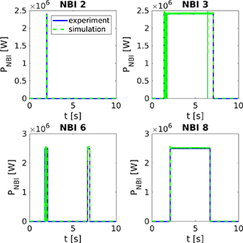
Figure 12. Time traces of the NBI power sources. The four different plots are for four different boxes. The experimental time trace is shown in blue, while the simulation one is shown in green. They overlap perfectly because the feedback on βp through NBI was switched off in order to validate the transport model, then the experimental time traces were used in the feed forward simulation.
Download figure:
Standard image High-resolution image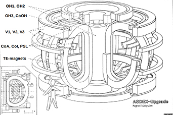
Figure 13. Geometry of the control magnetic coils of AUG.
Download figure:
Standard image High-resolution image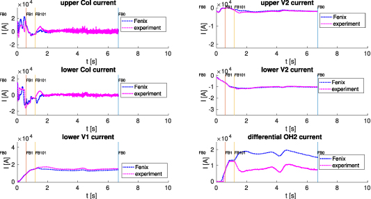
Figure 14. Time traces of some coil currents. The geometry of the coil currents is shown in figure 13. In all the plots, the experimental time trace is shown is purple, while the one from the simulation is shown in blue. Some vertical lines are shown in the plots to identify the beginning or the end of a feedback phase. One can see that different actuators act on different phases of the discharge: after the orange vertical line (i.e. during the ramp-up) all the coils are involved, while after the yellow vertical line (i.e. in the flat-top and ramp-down phases) only CoI and V2 control the shape and the position of the plasma. In fact, after this line, there is a sensitive difference between the differential of OH2 from experiment and and from simulation, because this actuator was not included in the feedback.
Download figure:
Standard image High-resolution image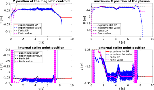
Figure 15. Time trace of some geometrical parameters of the plasma. These parameters are controlled by the coil currents shown in figure 14. The time trace of the DP used during the experiment is shown in red, the one used for real in the experiment is shown in blue, the DP used in Fenix is in black and the one used in the simulation is in purple. One can notice that for the maximum R position, the centroid Z position and the external strike point, the time traces overlap from 2 to around 7 s, which is during the flat-top, because a feedback is switched on.
Download figure:
Standard image High-resolution image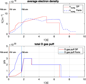
Figure 16. The upper plot shows the time trace of the electron density averaged along the entire radius, while the lower plot shows the time trace of the divertor gas puff, which is used to control the average density. In blue is the time trace from the simulation and in red the one from the DP. The orange vertical line represents the beginning of a feedback phase, while the blue one shows the end of it.
Download figure:
Standard image High-resolution image
Figure 17. Time traces of some global parameters of a Fenix simulation of the discharge #40446. (a) The plasma current, (b) illustrates q95, (c) is βp
and (d) is  (calculated as the average between
  and
and  ). The experimental trajectory is in red and the simulation is in blue..
Download figure:
Standard image High-resolution image
Figure 18. Time traces of some control parameters of the integrated model. In (a) the electron density at the separatrix is shown, in (b) the electron temperature at the separatrix is plotted, in (c) the ion power at the separatrix with its L–H threshold are plotted, in (d) βp at the top of the pedestal with its critical value is shown.
Download figure:
Standard image High-resolution imageIn figure 19 the kinetic profiles are shown for different phases of the discharge. Here, one can see that the profiles from the simulation are not within the experimental error bars, but for ρ < 0.9 the maximum error is  and for ρ > 0.9 it is
  . These errors show that the transport model can be improved, but we consider it a good starting point, considering that the task of the flight simulator is not a detailed analysis of the physics, but the prediction of the evolution of some global parameters. Considering that the discharge #40446 is an H-mode where the transition takes place at the beginning of the flat-top, one could argue that the mismatch in βp
found in the first 1.5 s is due to the fact that during this time range the plasma is in L-mode. In order to disprove this and disentangle the ramp-up from the L-mode, an additive Ohmic heated L-mode discharge (#38998) has been run in Fenix. The time traces of this discharge are shown in figure 20. Figure 21 shows the kinetic profiles between 2.4 and 2.7 s. Here on the right the density profile from Fenix (solid line) shows a non-negligible mismatch with the experimental one (dots). Such a disagreement deserves justification. The particle transport model used in the core is poor. An attempt to develop a more detailed and physics-based formula for the particle pinch matching TGLF in the simulations has been done, but it was not successful, therefore, the peaking factor cannot always be guaranteed. Moreover, this discharge is an L-mode, which is harder to predict, due to the absence of a pedestal model in the edge. It is worth mentioning that there is no inconsistency between the line averaged density time trace and the underestimation of the density profile, because there is no density feedback in this discharge.
. These errors show that the transport model can be improved, but we consider it a good starting point, considering that the task of the flight simulator is not a detailed analysis of the physics, but the prediction of the evolution of some global parameters. Considering that the discharge #40446 is an H-mode where the transition takes place at the beginning of the flat-top, one could argue that the mismatch in βp
found in the first 1.5 s is due to the fact that during this time range the plasma is in L-mode. In order to disprove this and disentangle the ramp-up from the L-mode, an additive Ohmic heated L-mode discharge (#38998) has been run in Fenix. The time traces of this discharge are shown in figure 20. Figure 21 shows the kinetic profiles between 2.4 and 2.7 s. Here on the right the density profile from Fenix (solid line) shows a non-negligible mismatch with the experimental one (dots). Such a disagreement deserves justification. The particle transport model used in the core is poor. An attempt to develop a more detailed and physics-based formula for the particle pinch matching TGLF in the simulations has been done, but it was not successful, therefore, the peaking factor cannot always be guaranteed. Moreover, this discharge is an L-mode, which is harder to predict, due to the absence of a pedestal model in the edge. It is worth mentioning that there is no inconsistency between the line averaged density time trace and the underestimation of the density profile, because there is no density feedback in this discharge.
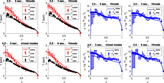
Figure 19. Kinetic profiles of a Fenix simulation of discharge #40446 for four time slots of the flat-top. The four plots on the left show in red (black) the electron (ion) temperature, where the solid line represents the simulation and the markers with the error bars represent the experimental profile. The four plots on the right show the electron density in blue, where the solid line represents the simulation and the dots with the error bars represent the experimental profile.
Download figure:
Standard image High-resolution image
Figure 20. Time traces of some global parameters of a Fenix simulation of the discharge #38898. (a) The plasma current, (b) illustrates q95, (c) is βp
and (d) is  (calculated as the average between
  and
and  ). In red is the experimental trajectory and in blue the simulation.
Download figure:
Standard image High-resolution image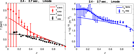
Figure 21. Kinetic profiles of the discharge #38898 between t = 2.4 and t = 2.7 s. On the left in red (black) is the electron (ion) temperature, while on the right in blue is the electron density. The solid line is the simulation while the dots are the experimental profiles with the error bars.
Download figure:
Standard image High-resolution imageA simulation including the match of the ramp-up phase is planned for the future. Finally, regarding the discharge #40446, in figure 22 the different contributions to χe via the ETG, ITG and TEM channels are shown along the entire discharge. One can see that, for this case, ITG is the dominant mode. In order to strengthen the validation of the integrated transport model, another four H-mode discharges with different particle sources and heating power time traces have been run. The trajectories of the plasma current and βp for the various discharges are shown in figure 23. Moreover, the time traces of the heating power and the D particle source for these discharges are compared respectively in figures 24(a) and (b), while the time trace of the average density of the core (for ρ < 0.3) is shown in figure 25. In figure 24(b) there is no gas puff signal for discharge #39977, because there was no diagnostic data available. One can notice that in figures 25(a), (c) and (d) there is an underestimation of the average density in the inner core (for ρ < 0.3). This is attributable to the particle transport model, which is not able to reproduce the peaking factor of the density. Moreover, the slow timescale of the simulated density reaction to the actuators does not allow us to reproduce a strong increase in the density in short times, as in figures 25(c) and (d). The feedback on the line averaged density for these discharges is switched off at around 1.5 s. All these results suggest that the model can predict the temperature profiles and the global parameter evolution, while some improvement is necessary to model the particle transport, especially in the presence of a strong concentrated increase in density and its peaking factor. Nevertheless, the main physics during the flat-top + ramp-down phase has been predicted, despite the differences between the various transients [73, 74]. This suggests that the transport model is appropriate for use in the usual AUG conditions in the Fenix suite.
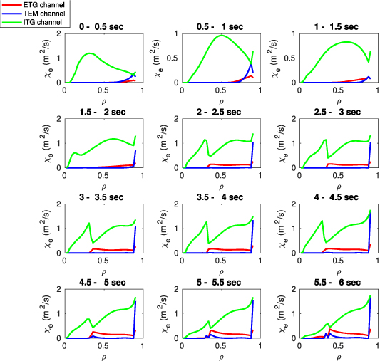
Figure 22. Contributions to the electron heat diffusivity from microturbulence during the entire discharge #40446. In red is the ETG contribution, in blue is the TEM part and in green is the contribution due to the ITG channel. One can see that the dominant contribution to the transport is due to the ITG mode.
Download figure:
Standard image High-resolution image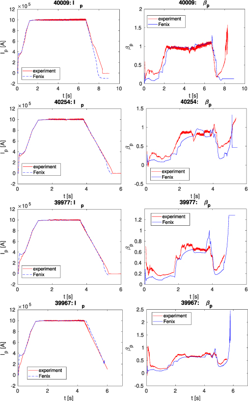
Figure 23. Time traces of Ip and βp for 4 H-mode discharges (#40009, #40254, #39977 and #39967). In blue is Fenix and in red is the experimental measurement.
Download figure:
Standard image High-resolution image
Figure 24. Time traces of the total heating power for 4 H-mode discharges are shown in (a), while the D gas puff is shown in (b). In (b) the experimental gas puff of the discharge #39977 is not shown because there was no diagnostic measurement of such a parameter.
Download figure:
Standard image High-resolution image
Figure 25. Time trace of the simulated (blue) and experimental (red) average density in the inner core (for ρ < 0.3) for the discharge #40009 in (a), #40254 in (b), #39977 in (c) and #39967 in (d). While for the pulse #40254 a good match is found, for the other three cases there is an underestimation of the density.
Download figure:
Standard image High-resolution image
6. Conclusions and future work
A set of analytical formulae that describe the transport in different plasma regions has been derived from theory-based models. For the core, some formulae from the literature have been fitted to TGLF+ASTRA simulations, to model temperature gradient-driven micro-instabilities. In the edge, an averaged ELM model has been used for the H-mode, coupled with Schmidtmayr scaling for the L-H transition, while in L-mode the core model has been extended to this region. For the SOL, two different models have been built to compute species densities and temperatures at the separatrix, respectively, based on a particle balance and the two-point model. Six discharges, five H-mode (#40446, #40009, #40254, #39977, #39967) and an L-mode (#38898), have been successfully simulated with the fully-integrated transport model in the Fenix flight simulator framework, and a match of the experimental trajectories during the flat-top and the ramp-down has been found, proving the ability to predict plasma energy and kinetic profile evolution with few experimental inputs. However, the ability to predict the peaking factor of the density profile is limited, thus some additional improvements to the particle transport must be investigated in the future. The analytical physics-based nature of the models allows us to use them in a realistic and fast way as a predictive tool. Their modularity opens up the possibility of constant updating by including new physical ingredients (e.g. detachment). The next step is the validation of the model against multiple AUG discharges in a wide range of configurations, and the extrapolation of it to machines of different sizes (e.g. ITER and DEMO). Long-term development also includes a physics-based modeling of the particle transport and the inclusion of a detachment model.
Data availability statement
All data that support the findings of this study are included within the article (and any supplementary files).
Acknowledgment
This work has been carried out within the framework of the EUROfusion Consortium, funded by the European Union via the Euratom Research and Training Programme (Grant Agreement No. 101052200 - EUROfusion). Views and opinions expressed are, however, those of the author(s) only and do not necessarily reflect those of the European Union or the European Commission. Neither the European Union nor the European Commission can be held responsible for them.