
Abstract
The intermittent behavior of a quasi-coherent density fluctuation is observed in a laboratory plasma. The quasi-coherent fluctuation is localized but intermittent events are observed in the whole region of plasma. Conditional averaging shows the intermittent events propagate from the central region of the magnetized plasma column to the peripheral region. Auto-correlation function of fluctuations and Hurst analysis reveal the intermittency is highly auto-correlated and the Hurst parameter reaches to 0.8, indicating the existence of self-similar behavior and long-range time correlation, and self-organized criticality dynamics might be the mechanism. Cross-bicoherence between different radii shows the nonlinear coupling between the quasi-coherent fluctuation and ambient turbulence, which will contribute to the generation of intermittency of turbulence.
Export citation and abstract BibTeX RIS

Original content from this work may be used under the terms of the Creative Commons Attribution 3.0 licence. Any further distribution of this work must maintain attribution to the author(s) and the title of the work, journal citation and DOI.
1. Introduction
A magnetically confined plasma is one of the systems far from equilibrium and thus exhibits dynamical behavior, and plasma turbulence is a key issue for understanding plasma dynamics. Turbulence intermittency, which is the enhanced particle bursts propagating across the open magnetic field region, has been observed in space plasmas [1, 2], fusion plasmas [3–9], and laboratory plasmas [10, 11]. The studies on intermittency reveal that it has a significant influence on plasma, which increases the radial non-diffusive transport and leads to flat density and temperature profiles [12, 13]. As a result, the 'main chamber recycling regime' can be dominant [14, 15] and the divertor efficiency is reduced. Besides, the intermittency can also increase the interaction of plasma with vacuum wall and thus enhance the erosion of the wall [16]. Furthermore, intermittency may also have a relation with the density limit of the discharge [17]. In order to reveal the underlying physics of intermittent turbulence, different statistical methods have been developed, including probability distribution function (PDF), conditional averaging analysis and Hurst parameter calculation [9, 11, 18–20]. The intermittency is found to behave with self-similar characteristic and long-range correlations, and self-organized criticality (SOC) like mechanism or avalanche dynamics [18, 21–24] have been proposed to explain intermittent turbulence events. However, the exact origin of turbulence intermittency still remains unclear, and further experimental evidence should be provided to reinforce the picture of it.
Laboratory plasma is very useful to study the turbulent intermittency, because it has excellent reproducibility and controllability and allows multi-point simultaneous measurement. This study was made to reveal the generation mechanism of the turbulence intermittency through the laboratory plasma experiment. Recently, a quasi-coherent fluctuation has been excited in the central region of linear magnetized laboratory plasma in the PANTA device through a large density gradient. The fluctuation is nonstationary and its amplitude varies in time intermittently. The impact of the intermittent event is observed in the whole plasma region, including the peripheral region where the density gradient is weak. This paper provides experimental results indicating a role of SOC dynamics in intermittency and correlation between intermittency and quasi-coherent fluctuation, and the paper discusses the generation mechanism of the turbulence intermittency.
2. Experimental setup
The experiment is performed in a linear device PANTA [25]. The PANTA is a 4-meter-long cylindrical device. The axial magnetic field, which is almost constant along the axis, is 0.09 T. The working gas is argon and the injected neutral argon pressure is 1 mTorr. Plasma is produced by a helicon wave (
 ) with a pulse duration of 500 ms. The center electron density, electron temperature and ion temperature of the plasma are approximately
 and
and  respectively.
The main diagnostic system used in this experiment is a frequency comb microwave reflectometer [26], which is installed at 1 meter in the axial direction as shown in figure 1(a). The reflectometer operates in ordinary mode (O-mode), and has 29 frequency channels, ranging from 12 GHz to 26 GHz with an interval of 0.5 GHz, which means that it can measure the density ranging from  to
to  The power spectrum density (PSD) of the incident wave is shown in figure 1(b). In this experiment, the microwave reflectometer starts the data acquisition from 100 ms of the discharge. Figure 1(c) shows the signal of the ion saturation current obtained by a 64-channel probe array at the mid-plane of 1875 mm in the axial direction and indicates that the plasma is stationary at the time during which the reflectometer collects data, as the red dashed lines denote. The reflected and incident waves are obtained and the phase delay between them is thus calculated, which indicates the time-of-flight of the wave. The equilibrium density profile is reconstructed by using time-of-flight and phase delay of each frequency component.

Figure 1. (a) Schematic of PANTA and the comb microwave reflectometer, (b) power spectrum density of the reflectometer incident wave, and (c) the ion saturation current obtained by the probe.
Download figure:
Standard image High-resolution imageIn working with phase, it is necessary to consider the ambiguity of  because the obtained phase difference is usually restricted in (
 ), here m is the arbitrary integer number. To solve this problem, we initialized the location of the center cut-off layer (corresponding to the channel with the highest frequency) based on the density profile measured with the Thomson scattering system, and the density profile is reconstructed by using the assumption that the differences of distance between two adjacent cut-off layers corresponding to comb frequency components are smaller than the wavelength of each comb component (
 ). Besides, a frequency comb sweep microwave reflectometer has been developed to eliminate the half-wavelength ambiguity of the cut-off layers [27] and the density profile is modified according to the one measured with the comb sweep reflectometer at the same experiment condition. The modified density profile along with those measured by the comb sweep reflectometer and Thomson scattering system are shown in figure 2. These three profiles agree well with each other, and all of them reveal an extremely large density gradient at around

Figure 2. Electron density profiles measured by reflectometers and Thomson scattering system.
Download figure:
Standard image High-resolution imageMeanwhile, the fluctuation of electron density, or in other words the density cut-off layer, causes perturbation of phase delay  Since no radial-coherent fluctuation is expected in the low density gradient region, and the irregular density burst has a radially elongated structure (shown later), the radial wavenumber (kr) is considered to be close to zero, which satisfies the small radial wavenumber condition (
 where kin is the wavenumber of the incident wave and LN is the density gradient length) [28, 29]. In this case, the back-scattering from such low-kr structures in this region is weak and has little effect on the reflected wave from the cut-off layer. In the large-gradient region where quasi-coherent fluctuation is easily excited, the back-scattering occurs and leads to an increase in the error of radial location. However, as such a structure is localized inside the narrow large-gradient region (discussed later), the error bars of the locations are almost the same as those of the density profile, which are shown in figure 2. Therefore, the effect of back-scattering can be neglected in our study, and the phase perturbation
  can be used to study the characteristics of density perturbation.
3. Characteristics of the quasi-coherent fluctuation
The quasi-coherent fluctuation observed in the PANTA is first characterized. The time-frequency spectrum and PSD of  at
at  which is proportional to the PSD of electron density fluctuation, are calculated and shown in figure 3. The frequency spectrum varies in time and two different frequency components are visible in the long-time averaged spectrum. These two components repeat growing and dumping irregularly. The low frequency component (
 ) is drift wave instability. We call the high frequency component (
 ) quasi-coherent fluctuation hereafter. This quasi-coherent fluctuation is only excited in the case of high power heating (
 ), and has a higher frequency than the drift wave frequency (which is usually
  ).
).
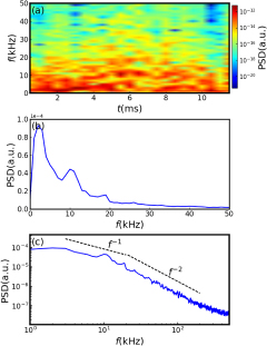
Figure 3. (a) Time-frequency spectrum of phase delay perturbation. Power spectrum density of phase delay perturbation in (b) linear and (c) log-log coordinates.
Download figure:
Standard image High-resolution imageMoreover, figure 3(c) shows the power spectrum in the whole frequency domain in the log-log plot, which is similar with other experimental observations [30, 31]. Different regions of power spectra scale as power lows, indicating correlations on different timescales. The f−2 decay of the power spectrum indicates a temporal process composed of uncorrelated increments (e.g. Brownian motion) [22, 32]. Actually, in the magnetized plasma turbulence, the high-frequency components (scaled as f−2) in the time series correspond to small-size transport events. Meanwhile the f−1 decay of the power spectrum is the distinctive feature of processes with long-range temporal correlations and often appears in conjunction with avalanche-like dynamics [21, 22]. In the PANTA, the f−1 decay of the power spectrum indicates a correlation between large-scale bursts and small-scale fluctuations. Owing to a similarity between the temporal and spatial spectra of turbulence in magnetized plasma, it is considered that spatial spectra of the PANTA plasma also indicate the power laws within the corresponding range. These power laws are important signatures of the SOC systems [22].
The radial structure of the quasi-coherent fluctuation is shown in figure 4. Figure 4(a) is the radial profile of the PSD of  at the frequency of 11 kHz. It shows that the strongest fluctuation is located between
  and
and  (denoted by the pink region), where the density gradient is largest as well. It is noted that the fluctuation strength decreases rapidly at the boundary of the large density gradient region. In addition, the formation of the strong gradient and excitation of the localized 11 kHz fluctuation in this region are confirmed by the Langmuir probe measurement [33]. Thus, it is reasonable to conclude that the fluctuation is excited by the gradient. Figure 4(b) is the radial wavenumber (kr) spectrum, which is obtained by calculating the cross phase of two radial channels at
  and
and  [34]. In this analysis, the time window is 1 ms and 23 ensembles with an overlapping of 0.5 ms are used. The kr is normalized by an ion sound Larmor radius
  (
( in the PANTA). Figure 4(b) reveals an extremely large wavenumber of the quasi-coherent fluctuation, which is around −5, indicating that the fluctuation has a small scale and is a pure inward propagating mode rather than a standing wave propagating in two opposite directions. This may help to identify the fluctuation, however, what the quasi-coherent fluctuation is still remains unknown now.
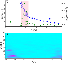
Figure 4. (a) Profile of phase delay fluctuation strength at  and (b) the radial wavenumber spectrum of the fluctuations.
Download figure:
Standard image High-resolution image4. Evaluation of intermittency
An intermittent density burst is also observed in this experiment. The spatiotemporal evolution of  is shown in figure 5. In the region of
  the amplitude of
  is dominated by the quasi-coherent fluctuation. The amplitude of the quasi-coherent fluctuation changes abruptly with a short timescale (∼0.1 ms). It is observed that sudden increases/decreases in the amplitude of the
  are radially synchronized beyond the outward boundary of the quasi-coherent fluctuation. There is a phase jump around
  close to the outward boundary of the quasi-coherent fluctuation. A ballistic propagation or avalanche-like propagation can be observed at the outer region. A decrease of
  starts from around 6.1 ms, and propagates from the central region (
 ) to the peripheral region (
 ), indicating the intermittent burst is a global event. It is noted that a decrease in the phase (i.e. the distance between the antenna and cut-off layer shortens) denotes an increase in the local electron density. The density burst originates from the outward boundary of the quasi-coherent fluctuation region, which indicates that the fluctuation may contribute to the generation of intermittency. It is also noted that the
  associated with the intermittent event in the peripheral region (
 ) has an anti-phase to the
  in the quasi-coherent fluctuation region.

Figure 5. Spatial-temporal evolution of phase delay perturbation.
Download figure:
Standard image High-resolution imageTo investigate the transport of intermittency, it is necessary to separate the intermittent bursts from background turbulence. Conditional averaging analysis is an important tool to extract these intermittent features and to reduce the effect of background perturbations, and the process is as follows [19]. A reference signal is selected and the threshold is set (usually several times of the root-mean-square (RMS) of the reference signal). The intermittent events that have a larger value than the threshold are thus discriminated, and the maxima (or minima) peaks of each event are detected. After setting a time window for averaging, the time series data with the length of time window around the maxima (or minima) are detected. Conditional averaging is achieved by accumulating and averaging the detected data. If the maxima (or minima) detection and data averaging are applied on the same signal, then it is called auto-conditional averaging, otherwise it is called cross-conditional averaging [3]. Auto- and cross-conditional averaging analysis allows us to simultaneously extract and average the intermittent bursts at different radii at the same timing, thus the spatial-temporal evolution of intermittency can be studied.
In this experiment, a threshold of  of
of  at
at  is used to detect the intermittent events. The time window is set as 160 μs, which is several times the decorrelation time (discussed later). Besides, we have made sure that the peaks of selected events are separated by at least 80 μs to avoid overlapping the two adjacent bursts. Auto- or cross-conditional averaging is thus performed to all channels, and the result is shown in figure 6. Similar with figure 5, phase delay decreases, i.e., density increase is observed and formed in the central region and propagating outward in the peripheral region, indicating the global structure of the intermittency. Figure 6 also reveals that the outward propagation velocity of the density bump is approximately 1 km s−1, which is consistent with the results in other devices [5, 6, 11]. It is also noted that inside
  the phase delay increases before intermittency bursts, indicating that the density hole is generated in the inner region before outward propagation of the density bump.
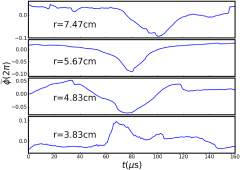
Figure 6. Conditional average of  at different radii.
Download figure:
Standard image High-resolution imageIntermittent behavior in the outer region ( ) is correlated to the abrupt increase in the amplitude of quasi-coherent fluctuation excited in the inner region (
 ). Figure 7 gives the radial correlations of
  Figures 7(a) and (c) show the cross-power spectrum density (CSD) at inner-outer and outer-outer regions respectively, and figures 7(b) and (d) are the corresponding squared radial coherence. The strong radial correlation at the mode frequency of 11 kHz is clearly shown across the phase inversion layer (figure 7(b)) and also at 2–3 cm far away from the phase inversion layer (figure 7(d)).
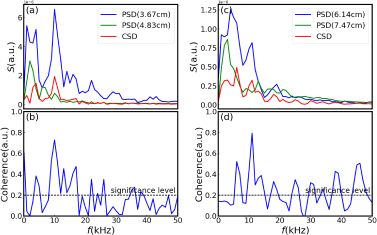
Figure 7. Auto- and cross-power spectrum densities of phase delay perturbations at (a) inner-outer regions and (c) outer-outer regions. (b) and (d) are corresponding coherences.
Download figure:
Standard image High-resolution imageThe SOC dynamics may play a role in the intermittent transport [3], and long-range time correlation (also called 'long-term storage' or 'persistence') is the key ingredient of the SOC behavior, which can be studied via autocorrelation function (ACF). The ACFs of phase delay perturbations at  and
and  are shown in figure 8. The dashed lines are eye-guide lines (exponential decay:
  and Lorentzian-like long tail:
  ). It can be seen that the decorrelation time of density fluctuation at
  which is the time lag for local ACF decaying lower than
  (see red dashed line), is approximately 40 μs. The ACF at
  shows a narrow peak when the time lag is smaller than 40 μs and a slow decay when the time lag is longer than 40 μs, indicating the existence of a long-range correlation. In contrast, the ACF measured at
  drops rapidly with time and shows no long tail.

Figure 8. Autocorrelation functions of phase delay perturbations at different radii.
Download figure:
Standard image High-resolution imageHowever, it is not easy to accurately determine the long-range correlation via the tail of ACF. A typical parameter for evaluating the long-range correlation is called Hurst exponent (H) [35], which expresses the scale of the long-range increasing of a time series data. According to [34], H ranges from 0 to 1.  indicates that there is long-range time correlation, while
  indicates long-range anticorrelation. If
  the process is an uncorrelated random process. The most commonly used method to calculate H is rescaled range (
 ) analysis [36, 37]. Here
  stands for the cumulated range (R) of a time series data over its standard deviation (S), and H is obtained by calculating the scale of
  with time.
However, it is basic to test the stationarity of the data samples before calculating H [28, 38], which cannot be accomplished with  analysis. Therefore, we started the test with structure function (SF) analysis. The structure function
  is defined as follows:

where x is a time series data of signal of interest, τ is the time lag, q is the order of structure function, i denotes the ith time point and  denotes the ensemble average. If the signal is stationary, then
  should be constant.
Figure 9(a) shows the SFs for different orders ( ) of the phase delay perturbation
  at
at  It is clear that
  is approximately constant with zero slope for all orders for
  between 50 μs and 3 ms, which indicates that the data is stationary. The
  method is used to calculate the Hurst component. Figure 9(b) is the
  values of
  versus time lag at
  From figure 9(b) it is shown that there is a transition at time lag
  For time lags smaller than 50 μs, the slope of linear fitting of
  values gives a Hurst exponent of about
  This large H is due to the non-stationarity of phase perturbation and should be neglected. For larger time lags (
 ),
),  is determined from the slope of
  values.
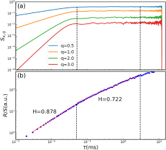
Figure 9. (a) Structure functions and (b)  analysis for density fluctuation.
Download figure:
Standard image High-resolution imageAfter calculating H of all channels, the radial profile of Hurst exponents is obtained and presented in figure 10. It is clear that at the region where the quasi-coherent fluctuation is located ( denoted by the pink region), the Hurst exponent is larger than 0.7, and the largest Hurst exponent reaches around 0.8. In contrast, the Hurst exponents out of
  are mostly between 0.6 and 0.7. This result indicates that the density bursts at the quasi-coherent fluctuation region have a long-range time correlation and SOC dynamics exist in this region. Since the intermittency originates from the outward boundary of this region (figure 5), it is thus reasonable to speculate that the origin of intermittent density burst propagation is driven by SOC dynamics when the critical threshold is reached due to the quasi-coherent density fluctuation.
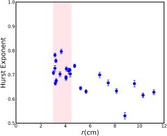
Figure 10. Profile of the Hurst exponent.
Download figure:
Standard image High-resolution image5. Nonlinear coupling with ambient turbulence
For intermittent events, another important property is the interplay between large- and small-scale fluctuations. Behaviors of the ambient turbulence are thus studied. The spatial and temporal scales of turbulence, which is obtained by a Bessel filter with bandpass frequency from 20 kHz to 50 kHz, are considered to be smaller and shorter than those of quasi-coherent fluctuation. Here the frequency range of the turbulence is determined based on the range where the power spectrum is scaled as  (figure 3(c)), i.e. the micro-turbulence range. Besides, after testing several different ranges between 20 kHz and 100 kHz, we found that the turbulent behaviors are almost the same. The envelope of this micro-turbulence is thus calculated with Hilbert transform, as shown in figure 11. The power spectra and coherence of envelopes of ambient turbulence at
  and
and  are given in figures 12(a) and (b), respectively.

Figure 11. Phase delay fluctuation (blue lines) and envelope (red lines).
Download figure:
Standard image High-resolution image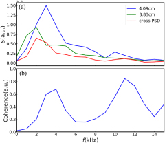
Figure 12. (a) Auto- and cross-power spectrum densities and (b) the radial coherence of the density fluctuation envelopes.
Download figure:
Standard image High-resolution imageIt is clear that even though the spectra are relatively weak, the cross-coherence of the turbulence envelope is significant at the frequency corresponding to the quasi-coherent fluctuation ( ), which suggests that the ambient turbulence closely correlates to the quasi-coherent fluctuation and the radial nonlinear coupling with the quasi-coherent fluctuation is thus worth investigating. Correlation with low frequency waves (
 ) are also suggested but the low frequency modes seem not to have long radial correlation, as discussed later.
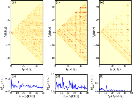
To reveal the relationship between ambient turbulence and intermittency, the two-point cross-bicoherence, which is an index of multi-scale coupling at different radii, are calculated [39–41]. The two-point cross-bicoherence is defined as
where X is the Fourier representation of time series data x and B is the two-point cross-bispectrum defined as

where  denotes the complex conjugate of X. The summed two-point cross-bicoherence is written as

where N is the number of the elements satisfying  We calculated two-point cross-bicoherences in the inner region (
 and
and  ), in the outer region (
 and
and  ) and across the phase inversion layer (
 and
and  ) by using the phase delay perturbation
  at these radii and they are shown in figures 13(a), (c) and (e), and the corresponding summed two-point cross-bicoherences are shown in figures 13(b), (d) and (f), respectively. In the inner region, strong nonlinear three-wave coupling between ambient turbulence (20–50 kHz) and the quasi-fluctuation
  is visible. This means that the ambient turbulence is modulated by the quasi-coherent fluctuation. Although turbulence modulation at lower frequency is suggested in figure 12 and summed two-point cross bicoherence is significant in the low frequency range, there is no clear peak in the low frequency range, as shown in figure 13(b). The turbulence modulation is also observed in the outer region. The summed two-point cross-bicoherence at
  is larger than that observed in the inner region. A small but clear peak is present in figure 13(e). This indicates that nonlinear coupling between ambient turbulence and the quasi-coherent fluctuation across the phase inversion layer exists. A plausible conclusion is that the nonlinear three-wave coupling between the micro-turbulence and the quasi-coherent meso-scale structure correlates global or long-range behavior of the intermittent event.
Figure 13. Two-point cross-bicoherences of phase fluctuations at (a)  and
and  (c)
(c)  and
and  (e)
(e)  and
and  (b), (d) and (f) are corresponding summed cross-bicoherences.
Download figure:
Standard image High-resolution image
By now, we can have a physical view of the intermittency generation according to the results above. A quasi-coherent fluctuation is firstly excited by the large density gradient, which perturbs the background density. The initial positive and negative density bursts are formed and propagate outward and inward, respectively, due to the SOC dynamics when the critical threshold is reached. Because of the nonlinear three-wave coupling with the quasi-coherent fluctuation, the distant turbulence, which means the turbulence in the peripheral region and radially far away from the quasi-coherent fluctuation, is modulated, which enhances the radial correlation of density bumps and extends the ballistic radial propagation. The radial-scale of the burst propagation is thus elongated and the global intermittency is generated.
Identification of the quasi-coherent fluctuation and discussion of avalanche-like transport behavior are left for future work. Reflectometry in conjunction with multi-probe systems will give more details of the spatial structure of the quasi-coherent mode. In order to identify the avalanche transport [21–24], simultaneous measurement of temporal evolution of density gradient is required. Fast reconstruction of the density profile by using the microwave frequency comb reflectometer is one of the promising methods. Such a fast reconstruction method is under development.
6. Summary
In order to understand intermittency of turbulence and its impact on transport in magnetized plasma, the intermittent behavior of quasi-coherent density fluctuation and associated radial propagation of density bump/hole in the whole measured plasma region are investigated experimentally. A quasi-coherent fluctuation ( ) is excited in the narrow steep density gradient region (
 ) in the PANTA. An abrupt change in the amplitude of the quasi-coherent fluctuation accompanied by global radial propagation of the density bump in the peripheral region (
 ) is identified. To observe long-term storage, long-range correlation and self-similarity of fluctuations, signal processing and data analysis are performed and results indicate: (i) the autocorrelation function of fluctuations displays a long tail at the inner region (
 ) and (ii) the Hurst exponent is much larger than 0.5 (
 ) at the quasi-coherent fluctuation region, indicating that the intermittency is highly auto-correlated and has long-range memory, which resembles that in a SOC system. (iii) Finite cross-bicoherences between two-distant locations are observed, which means there is nonlinear long-range coupling between ambient turbulence and the quasi-coherent fluctuation. The generation mechanism of intermittency is accordingly revealed. The background density is perturbed by the high-frequency quasi-coherent fluctuation, which is excited by the large density gradient. When the critical threshold is reached, the radial propagation of the density burst can be triggered due to the SOC dynamics. The distant turbulence, which is coupled with the quasi-coherent fluctuation, enhances the radial correlation of density bursts. It can elongate the radial propagation and can form the global intermittency. The observed intermittent behavior of turbulence and its characterization will have deep impact on our predictability of the evolution of turbulent plasmas.
Acknowledgements
This work is supported by JSPS KAKENHI Grant Numbers 15H02335, JP17H06089.