Sensitivity volume as figure-of-merit for maximizing data importance in electrical impedance tomography

Consider the full model space ${{\mathfrak{M}}}_{{\mathfrak{0}}}$ of the EIT problem with dimension M₀. Typical EIT inverse methods parameterize this full model space as a mesh defined over the volume of interest, with one independent model coordinate per mesh piece. Our strategy will be instead to choose a much smaller model subspace ${\mathfrak{M}}\subset {{\mathfrak{M}}}_{0}$ with dimension M ≪ M₀ spanned by orthogonal basis functions comprised of linear combinations of these mesh pieces and designed to target the features of interest. Prior knowledge of the system can be used either to identify the most important features, for example, with proper orthogonal decomposition (POD) (Lipponen 2013), or, alternatively, to provide balanced resolution throughout, for example, with a harmonic polynomial series appropriate to the geometry of interest, such as Legendre polynomials, Zernike polynomials, or Fourier decomposition.

Whereas standard EIT methods use the number of contacts C to fix the dimension D of the data space ${\mathfrak{D}}$, here an increased contact number C₀ will be used to define a larger data space ${{\mathfrak{D}}}_{0}$ of dimension D₀ greater than strictly necessary. Inside this expanded data space, an optimal subspace ${\mathfrak{D}}\subset {{\mathfrak{D}}}_{0}$ of dimension D < D₀ can be found, according to the steps in the following section. Note that under this method, contacts do not have to be equally spaced around the periphery, but can be placed arbitrarily, for example with higher density near features of interest, though for most common applications the need for uniform resolution dictates equal spacing of contacts.

Consider the dimensionality D of a desired data space and the corresponding minimum number of contacts C that spans that data space (Brown and Seagar 1987),

$$\begin{eqnarray}&&D=\displaystyle \frac{C(C-3)}{2},\end{eqnarray} \tag{ 8 }$$

which can be inverted to yield the equivalent relation,

$$\begin{eqnarray}&&C=\unicode{x02308}\displaystyle \frac{3}{2}+\sqrt{\displaystyle \frac{9}{4}+2D}\,\unicode{x02309}.\end{eqnarray} \tag{ 9 }$$

Here the ceiling function ⌈ · ⌉ ensures an integer number of contacts.

Since advantages of the sensitivity volume method come from increasing the dimensionality of the data space and therefore increasing the contact number, it is important to quantify what increase in contact number corresponds to what increase in data space dimension. If the data space is expanded to dimension D₀ by a data space inflation factor r_D ,

$$\begin{eqnarray}&&{r}_{D}={D}_{0}/D,\end{eqnarray} \tag{ 10 }$$

the number of contacts must increase to C₀.

$$\begin{eqnarray}&&{C}_{0}({r}_{D})=\unicode{x02308}\displaystyle \frac{3}{2}+\sqrt{\displaystyle \frac{9}{4}+2\,{r}_{D}D}\,\unicode{x02309}.\end{eqnarray} \tag{ 11 }$$

This increase can be represented with a contact number inflation factor r_C ≃ C₀/C, which can be determined from the above equations:

$$\begin{eqnarray}&&{r}_{C}=\displaystyle \frac{3}{2C}+\sqrt{{r}_{D}-\displaystyle \frac{3{r}_{D}}{C}+\displaystyle \frac{9}{4{C}^{2}}}.\end{eqnarray} \tag{ 12 }$$

Note that with a large number of contacts, the relation between r_D and r_C simplifies to ${r}_{D}\sim {r}_{C}^{2}$ meaning that the data space inflates roughly quadratically with the contact number.

The larger the data space inflation factor r_D , the likelier the inflated data space of dimension D₀ = r_D D can contain a subspace of desired dimension D that includes only the most independent and noise-robust measurements. Note that the total number of possible four-point measurements D_max that can be made with arbitrarily chosen contacts is of order ${ \mathcal O }({{C}_{0}}^{4})$:

$$\begin{eqnarray}&&{D}_{\max }({C}_{0})=\displaystyle \frac{{C}_{0}!}{({C}_{0}-4)!},\end{eqnarray} \tag{ 13 }$$

thus the search space for optimization increases geometrically with the contact number. We will refer to the list of all D_max possible four-point data measurements as the measurement library, from which D measurements will be chosen to form the candidate protocols.

Having identified the model space ${\mathfrak{M}}$, the contact number and placement, and the full data space ${{\mathfrak{D}}}_{0}$ with total number of possible measurements D_max, the Jacobian can now be calculated from the forward problem. Let each row of the Jacobian matrix J represent a sensitivity vector μ _a in model space, composed of the sensitivity coefficients defined in equation (4),

$$\begin{eqnarray}&&{{\boldsymbol{\mu }}}_{a}=[{J}_{a1},{J}_{a2},\,\ldots ,\,{J}_{{aM}}].\end{eqnarray} \tag{ 14 }$$

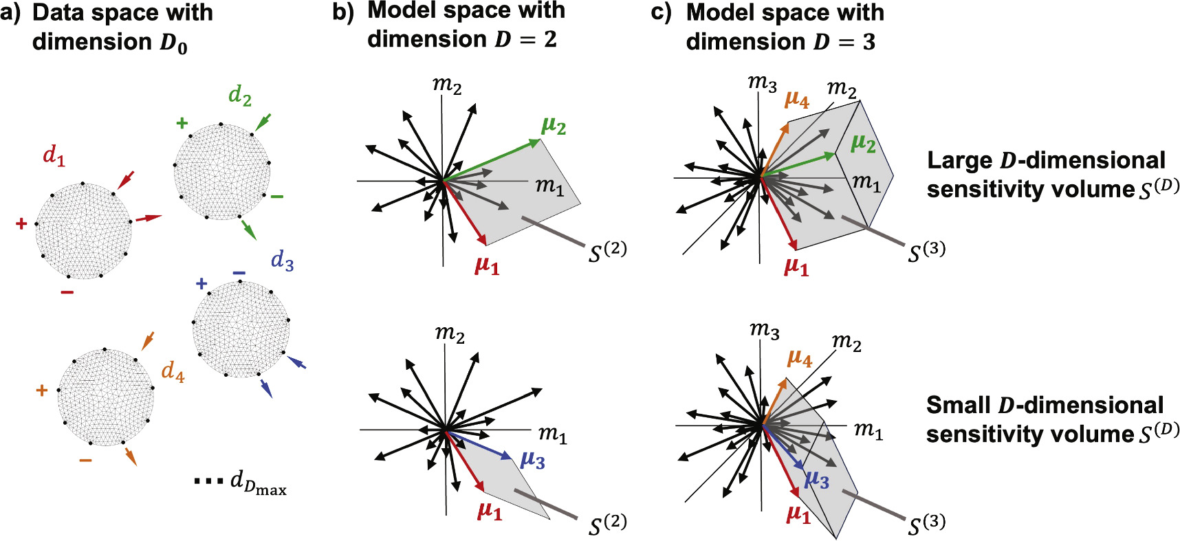
As illustrated in figure 1, each sensitivity vector represents the overall sensitivity of the a^th data measurement $a=\{1...{D}_{\max }\}$ to the set of β = {1... M} orthonormal basis functions of the chosen model space. The overall sensitivity of a given measurement is thus proportional to the magnitude of its sensitivity vector.

Zoom In Zoom Out Reset image size

The sensitivity volume is the key figure-of-merit introduced here in order to compare and optimize choice of candidate measurement protocols. The sensitivity of a set of D independent measurements selected from the library of D_max available measurements can be quantified as the D-dimensional volume S^(D) of a parallelotope subtended by the chosen α = 1 ... D sensitivity vector rows of the Jacobian matrix:

$$\begin{eqnarray}&&{S}^{(D)}=\sqrt{\det ({{\bf{JJ}}}^{{\mathsf{T}}})},\end{eqnarray} \tag{ 15 }$$

as illustrated in figure 1. Conceptually, the sensitivity volume can be thought of as the product

$$\begin{eqnarray}&&{S}^{D}=\displaystyle \prod _{\alpha =1}^{D}| {{\boldsymbol{\mu }}}_{\alpha \perp }| ,\end{eqnarray} \tag{ 16 }$$

where μ _α⊥ is the perpendicular component of sensitivity vector α with respect to all other vectors in the set. This result is also identical to the product of the α = {1 ... D} singular values s_α of the SVD decomposition:

$$\begin{eqnarray}&&{S}^{\left(D\right)}=\displaystyle \prod _{\alpha =1}^{D}{s}_{\alpha }\,.\end{eqnarray} \tag{ 17 }$$

The geometric mean S of the singular values s_α is then the average sensitivity per measurement in the data space, or the Dth root of the D-dimensional sensitivity volume, henceforth referred to as the specific sensitivity or in appropriate context simply the sensitivity of that measurement protocol:

$$\begin{eqnarray}&&S=\sqrt[D]{{S}^{(D)}}.\end{eqnarray} \tag{ 18 }$$

The data space ${\mathfrak{D}}$ will be chosen to have dimension D that matches that of the model space D = M, setting up an exactly determined inverse problem. The underdetermined case D < M would leave some of the desired model space features undefined, and the overdetermined case D > M would measure redundant information at the cost of computational efficiency and measurement duration. With the sensitivity volume figure-of-merit defined above, the strategy will then be to search for a data subspace ${\mathfrak{D}}\subset {{\mathfrak{D}}}_{0}$ with dimension D = M whose measurement protocol is selected from the measurement library to have maximal sensitivity volume S^(D) according to the chosen basis functions of our model space ${\mathfrak{M}}$.

In the exact determined linearized inverse problem considered here D = M, the Jacobian J is square and invertible such that J^−g = J⁻¹. This makes the inverse solve in the absence of data noise computationally efficient by eliminating the need for regularization, such as Tikhonov regularization, gradient damping, or total variation regularization (Holder 2005, Menke 2012). Because of the increase in sensitivity S under the sensitivity volume method, it is less likely that truncation of singular values will be required under SVD analysis, making direct matrix inversion adequate in many cases. But in the presence of noise that exceeds the Picard condition, a simple regularization procedure, such as truncated (T)SVD, can still remove the influence of small singular values overcome by noise (Hansen 1990a). And with the dimensionality of J greatly reduced, there remain significant improvements in computational efficiency over T(SVD) of a standard Jacobian.

To differentiate between two model cases under increasing data noise, we generalize the distinguishability criterion z proposed by Adler et al (2011), Yasin et al (2011) and also define a noise threshold for distinguishability η_t . Consider the noiseless inverse models {m_a, m_b} corresponding to two different model cases to be distinguished under noise. In the linear regime, noisy inverse solves will fall in a neighborhood around these models, described by the posterior model covariance matrix C_m :

$$\begin{eqnarray}&&{{\bf{C}}}_{{\bf{m}}}={{\bf{J}}}^{-g}{{\bf{C}}}_{{\bf{d}}}{{{\bf{J}}}^{-g}}^{{\mathsf{T}}},\end{eqnarray} \tag{ 19 }$$

where the data covariance matrix C_d = η² I represents, in this case, uncorrelated Gaussian experimental noise with standard deviation η, and I is the identity matrix. Whereas Adler et al identified a spatial cross-section of interest for statistical analysis, here the analysis will be conducted along a segment in model space that connects two model cases to be distinguished. A unit vector $\hat{{\bf{u}}}$ can be defined along this segment connecting the two noise-free models:

$$\begin{eqnarray}&&\hat{{\bf{u}}}=\displaystyle \frac{{{\bf{m}}}_{{\rm{b}}}-{{\bf{m}}}_{{\rm{a}}}}{| {{\bf{m}}}_{{\rm{b}}}-{{\bf{m}}}_{{\rm{a}}}| },\end{eqnarray} \tag{ 20 }$$

and the component of each model's covariance C_m projected along this direction is:

$$\begin{eqnarray}&&{\sigma }_{a}^{2}={\sigma }_{b}^{2}={\hat{u}}^{T}{C}_{m}\hat{u}.\end{eqnarray} \tag{ 21 }$$

Following Adler et al, the standard deviation of the model difference σ_m becomes

$$\begin{eqnarray}&&{\sigma }_{{\rm{m}}}^{2}={\sigma }_{{\rm{a}}}^{2}+{\sigma }_{{\rm{b}}}^{2}.\end{eqnarray} \tag{ 22 }$$

The result is a generalization of Adler et al's distingushability z in model space:

$$\begin{eqnarray}&&z=\displaystyle \frac{| {{\bf{m}}}_{{\rm{b}}}-{{\bf{m}}}_{{\rm{a}}}| }{{\sigma }_{{\rm{m}}}},\end{eqnarray} \tag{ 23 }$$

where z = 1 represents the threshold for distinguishability, and statistical significance is defined as z > 2 per mathematical convention (Cowan 1998).

A noise threshold η_t for distinguishability in the case of uncorrelated Gaussian noise can be determined by solving equations (19)–(23) according to the condition z = 1:

$$\begin{eqnarray}&&{\eta }_{t}^{2}=\displaystyle \frac{| {{\bf{m}}}_{{\rm{b}}}-{{\bf{m}}}_{{\rm{a}}}{| }^{2}}{2{\hat{{\bf{u}}}}^{T}({{\bf{J}}}^{-g}{{{\bf{J}}}^{-g}}^{{\mathsf{T}}})\hat{{\bf{u}}}}.\end{eqnarray} \tag{ 24 }$$

Noise exceeding this threshold renders cases {m_a} and {m_b} indistinguishable, i.e. within a standard deviation of noise of each other, and noise below half η_t means the two cases can be discerned with statistical significance.

According to the sensitivity volume method, one first chooses a reduced model space (M < M₀) that will have sufficient feature resolution. Given the circular symmetry of this test problem, the results of POD from Allers and Santosa (Allers and Santosa 1991) and from Lipponen et al (2013) suggest that Zernike polynomials shown in figure 2 defined over a mesh will provide an excellent empirical basis for model space parameterization. The orthonormal Zernike polynomial functions are defined on a unit disk in terms of polar coordinates ${Z}_{n}^{h}(r,\theta )$, with increasing radial order n = {0, ... N} and angular order h = { − n, − n + 2, ... n − 2, n} representing increasing resolution where N is the highest polynomial order of the Zernike polynomials used (Lakshminarayanan and Fleck 2011):

$$\begin{eqnarray}{Z}_{n}^{h}(r,\theta )=\left\{\begin{array}{ll}{F}_{n}^{h}{R}_{n}^{| h| }r\cos (h\theta ) & \mathrm{for}\,h\geqslant 0,\\ -{F}_{n}^{h}{R}_{n}^{| h| }r\sin (h\theta ) & \mathrm{for}\,h\lt 0,\end{array}\right.\end{eqnarray} \tag{ 25 }$$

where ${R}_{n}^{| h| }$ is defined as

$$\begin{eqnarray}&&{R}_{n}^{| h| }(r)=\displaystyle \sum _{l=0}^{\tfrac{n-h}{2}}\displaystyle \frac{{\left(-1\right)}^{l}(n-l)!}{l!\left(\tfrac{n+h}{2}-l\right)!\left(\tfrac{n-h}{2}-l\right)!}{r}^{n-2l}.\end{eqnarray} \tag{ 26 }$$

The normalization prefactor F_n ^h is

$$\begin{eqnarray}&&{F}_{n}^{h}=\sqrt{\tfrac{2(n+1)}{1+{\delta }_{h0}}},\end{eqnarray} \tag{ 27 }$$

where δ_h0 is the Kronecker delta function (Lakshminarayanan and Fleck 2011). Using this polynomial basis, any conductivity map can be represented as a linear combination of Zernike polynomials:

$$\begin{eqnarray}&&\begin{array}{l}\sigma (r,\theta )={\sigma }_{0}(r,\theta )+\displaystyle \sum _{n=0}^{N}\displaystyle \sum _{h=-n,-n+2,\ldots }^{n}{m}_{n,h}{Z}_{n}^{h}(r,\theta ),\end{array}\end{eqnarray} \tag{ 28 }$$

where σ₀(r, θ) is the reference, chosen here to be homogeneous.

Zoom In Zoom Out Reset image size

For a given polynomial order N, the dimension M_P of the polynomial model space up to and including that order is:

$$\begin{eqnarray}&&{M}_{{\rm{P}}}=\tfrac{(N+1)(N+2)}{2}.\end{eqnarray} \tag{ 29 }$$

In practice, the order N of the polynomial will be chosen large enough that M_P ≥ M, and the specific M polynomials for the model space basis are chosen to suit prior knowledge of electrode symmetries and the desired resolution of the problem at hand. Thus, the model conductivity m is represented here as a vector of length M describing the set of weights for each polynomial m_n,h .

To deploy these continuous basis functions in a finite element solver, Zernike polynomials (Fricker 2023) were projected onto a fine mesh generated in EIDORS with Netgen (Adler and Lionheart 2006). An M₀ × M-dimensional mapping matrix Z transforms the M-dimensional model vector m in the polynomial basis into a M₀-dimensional vector m^mesh on a finite element mesh,

$$\begin{eqnarray}&&{{\bf{m}}}^{\mathrm{mesh}}={\bf{Z}}\,{\bf{m}}.\end{eqnarray} \tag{ 30 }$$

The same mapping matrix Z maps a D × M₀-dimensional Jacobian J^mesh derived on a finite element mesh into a D × M-dimensional Jacobian J:

$$\begin{eqnarray}&&{{\bf{J}}}^{\mathrm{mesh}}\,{\bf{Z}}={\bf{J}},\end{eqnarray} \tag{ 31 }$$

where each of M columns of Z corresponds to the mesh-element parameterization of each continuous Zernike polynomial. As a result, the forward problem can be written as:

$$\begin{eqnarray}&&{\bf{d}}={\bf{Jm}}={{\bf{J}}}^{\mathrm{mesh}}{{\bf{m}}}^{\mathrm{mesh}}.\end{eqnarray} \tag{ 32 }$$

For the biomedical example of a 'normal' versus 'enlarged heart,' M = 27 independent standard Zernike polynomials of increasing resolution were chosen up through order N = 6. This uniform resolution model space is represented by all the polynomials plotted in figure 2 except for the bottom center n = 6; h = 0. For the engineering example comparing 3 versus 6 reinforcement rods, prior knowledge that the system of interest had either 3-fold or 6-fold rotational symmetry allowed the M = 27-dimensional model space to be constrained, accordingly. Here, this model space is represented by the first M = 27 standard Zernike polynomial functions that satisfy the 3- and 6-fold symmetry requirements, requiring the sampling of polynomials up to order N = 12. In both cases, a homogeneous constant background was used as a reference, and the higher conductivity test features were given a 20% enhancement in the conductivity.

For both examples, the contacts are equally spaced at the circumference with the number of contacts set according to equation (11). In order to have D = M = 27 measurements, we find for the adjacent measurement protocol that an uninflated r_D = 1 data space (and uninflated contact number r_C = 1) requires C₀ = C = 9 contacts. For the sensitivity volume measurement protocol, an inflated data space with r_D = 12 gives overall dimension D₀ = r_D D = 324 which requires C₀ = 3C = 27 contacts per equation (11). It is observed that when using Zernike polynomials as the model space basis, an odd number of contacts C₀ is preferred to minimize the null space at the maximum radial order n = N.

For the inflated data space with C₀ = 27 contacts, sensitivity vectors for both the biomedical and engineering examples were calculated per equation (14) for all ${D}_{\max }({C}_{0})=421,200$ possible measurements. These calculations used the default EIDORS forward solver with the adjoint Jacobian (Vauhkonen et al 2001, Adler and Lionheart 2006) on a homogeneous reference, along with appropriate mapping matrices Z per equation (30) for each scenario's model space. The resulting libraries of D_max sensitivity vectors formed measurement search spaces for the two respective cases.

Sensitivity volumes were determined for each case per equation (17) for various measurement protocols with D = M = 27 sensitivity vectors chosen from the library of D_max available. The sensitivity volumes are then compared to find which D out of D_max specific vectors maximizes the sensitivity volume figure-of-merit S^(D). Various search algorithms can be implemented such as a greedy search (Williamson and Shmoys 2011), genetic search (Press et al 2007), or simulated annealing (Press et al 2007) to find this measurement protocol with maximum sensitivity volume. In the examples below, a modified greedy search was implemented.

Table 1 shows the sensitivity volume optimized protocol for data space measurements for the biological and engineering scenarios, respectively. Just over half of these measurements (highlighted) have a similar configuration whereby the current injection electrode I⁺ neighbors the positive voltage V⁺ electrode, the current sink I⁻ neighbors the negative voltage V⁻, and the inner/outer pairs are of the same type, either current or voltage. Because the contacts of this frequent configuration are the same as an adjacent configuration but functionally rotated analogous to a Van der Pauw conjugate measurement (Van der Pauw 1958), this contact configuration will be referred to as the 'adjacent–conjugate' configuration. But it should be pointed out that the resulting measurements in the protocols do not follow a rotational symmetry like the adjacent or skip measurement protocols and could not have been empirically guessed in advance. Furthermore, the biological problem with its uniform resolution model results in a rather different measurement protocol than the engineering problem with its 3/6-fold constrained symmetry, illustrating the dependence of the measurement protocol on the model structure.

Table 1. Measurement protocols for the biomedical and engineering examples, with current injection between I⁺ and I⁻ electrodes and voltage measurement across electrodes V⁺ and V⁻. More than half the measurements (highlighted in grey) are of a similar configuration which we define to as 'adjacent–conjugate,' whereby each voltage electrode neighbors a current electrode, and the inner/outer pairs are current/voltage electrodes.

We reiterate that once an optimal measurement protocol is determined, there is no need to repeat the sensitivity volume optimization. Because the computationally intensive steps of sections 4.3 through 4.5 are performed in advance to generate the Jacobian for the optimized data space, the inverse solve can now be extremely rapid, as fast as a simple matrix multiplication.

To complete the sensitivity volume method, one must solve the resultant exact determined inverse problem (M = D). A Matlab code was written to use (truncated) singular value decomposition (T)SVD to solve the linearized, non-iterative inverse problem for orthogonal polynomial model spaces per equation (7). Data was simulated using EIDORS' default forward solver and a finite element mesh. Gaussian noise with standard deviation η was added to the simulated data to emulate realistic experimental conditions.

In the biomedical example, our SVD solver was used with no truncation of singular values. Figure 3(a) shows the 'input' conductivity maps in the forward problem for the 'normal' heart (top) and the 'enlarged' heart (bottom) using an EIDORS derived mesh. Reconstructed conductivity maps of the noiseless (η = 0) normal and enlarged heart are shown in color in the left of panel (b) for the standard adjacent measurement protocol, and the left of panel (c) for the sensitivity volume maximized measurement protocol. The polynomial model space in section 4.1 and the inverse solver described in section 4.6 were used to produce reconstructed images from simulated datasets using both measurement protocols. In the absence of noise, all reconstructions show similar resolution, with the exception that the enlarged case for the adjacent measurement protocol shows artifacts with residual oscillations at the periphery.

Zoom In Zoom Out Reset image size

To investigate noise tolerance, the mean results of 1000 simulated SVD inversions of normal and enlarged hearts were generated with increased data noise η. As noise increases to the right in figure 3, the standard adjacent measurements in the top rows generate average inverse maps that deviate further from the noiseless reconstructions, and eventually become overwhelmed by the noise. By contrast, reconstructions using sensitivity volume derived measurements in the bottom rows can withstand over an order of magnitude more noise than the adjacent measurements.

The results can be quantified using the distinguishability and noise tolerance metrics of Subsection 3.7. The distinguishability z was calculated at each noise level η for reconstruction of both adjacent and sensitivity maximized measurement protocols. The distinguishability threshold is defined as z = 1, whereupon the normal and enlarged cases become statistically indistinguishable, and η_t is the corresponding noise level threshold. For z > 1, the average inverse maps begin to show differences from the noise-free scenario, and z = 2 represents the threshold for statistically significant distinguishability (Cowan 1998). The noise threshold η_t for both cases is listed in table 2 and shows that the sensitivity volume maximized dataset tolerates a factor of 25 × more noise than the adjacent measurement protocol, with the same number of measurements. Table 2 also lists the increase in relative sensitivity S/S₀ of the sensitivity volume measurement protocol from equation (18) relative to that of the adjacent measurement protocol.

In the engineering example, our (T)SVD solver was used for both measurement protocols with a truncation point of k = 18 singular values, as necessitated by smaller amplitudes of the singular values from the Jacobian matrices. Figure 4(a) shows the forward problem input maps of 3 rods (top) and 6 rods (bottom). Reconstructed conductivity maps of the noiseless (η = 0) cases are shown in color in the left of panel (b) for the standard adjacent measurement protocol, and the left of panel (c) for the sensitivity volume maximized measurement protocol. Datasets generated using both measurement protocols were reconstructed using the 3- and 6-fold symmetric polynomial model space described in section 4.1. Once again, the mean results of 1000 (T)SVD inverse solves are generated with increasing noise η from left to right. In the reconstructions from adjacent measurements in panel (b), small singular values in the (T)SVD inversion cause the noise to rapidly overtake any meaningful model features. In contrast, sensitivity volume maximized measurements in panel (c), can withstand three orders of magnitude more noise before such model obfuscation occurs, with the respective η_t values again listed in table 2.

Zoom In Zoom Out Reset image size

The final advantage of the sensitivity volume method is to leverage the gain in sensitivity to achieve faster computational time. A rapid refresh rate for tomographic mapping is important in applications where the system under study is dynamically varying, such as a beating heart or a structural element under imminent failure. But when solving inverse problems in the presence of data noise, it is typically necessary to rely on an iterative solver which can slow down the inversion algorithm.

Here, a standard iterative solver is challenged against the non-iterative sensitivity volume method with the same distinguishability problem for the biomedical and engineering cases, above. The noise threshold, and its computation times were compared to the computation times of our non-iterative sensitivity volume method under the same noise level. The iterative solver to be compared is the publicly available EIDORS iterative Gauss Newton inverse solver (Adler and Lionheart 2006), which can conduct inverse solves in 100 or fewer iterations with the regularizing hyperparameter set to 1 × 10⁻⁷. For calculations of the EIDORS noise threshold, the model covariance was estimated from ensembles of 100 different inverse solves for different noise amplitudes η, and the resulting noise thresholds are listed in table 3. The noise threshold of the iterative EIDORS regularized inversion with the adjacent data space, is always of the same order of magnitude and slightly less than the noise tolerated by the non-iterative (T)SVD inversion with the sensitivity volume method. Table 3 shows the significant speed advantage of inverting with the non-iterative sensitivity volume method over inverting with a regularized, iterative solver by comparing their computation times t_c for the examples shown previously. The sensitivity volume method produces results in approximately 1/600 000^th the computation time of the EIDORS inverse solver.

In the sensitivity volume method, inflating the data space comes at a cost of adding more contacts. Thus, it is important to quantify the degree to which an inflation of the data space leads to an improvement in the overall sensitivity. A computational study of the sensitivity for a 2D circle was undertaken for various data space inflation factors r_D = 1, 3, 5, and 10 with equally spaced circumferential contacts, a homogeneous reference, and a Zernike polynomial model space, and the corresponding factor of increase in contact number r_C was compared.

In figure 5, the initial number of contacts C listed on the bottom axis will set the baseline data space dimension D per equation (8). Then this data space will be increased by the factor r_D to the value D₀, requiring that the contact number also be correspondingly increased to C₀(r_D ) listed along the top axis of figure 5 per equation (9). The inset of figure 5 compares the exact value by which the contact number is inflated C₀(r_D )/C (filled circles) along with the analytical expression for r_C from equation (12) (solid lines), showing good agreement. In particular, equation (12) predicts that the r_C factor saturates at ${r}_{C}=\sqrt{{r}_{D}}$ for large contact number (dashed horizontal lines), with this saturation evident already for C > 10.

Zoom In Zoom Out Reset image size

The sensitivity improvement S is then plotted on the vertical axis of figure 5 relative to the adjacent measurement protocol S₀. The behavior reveals significant increase in the sensitivity ratio S/S₀ by one-and-a-half orders of magnitude as the data space D₀ expands by increasing factors of r_D , and this enhanced sensitivity is most dramatic with the largest number of contacts. For convenience, the following empirical expression for the sensitivity enhancement can serve as a guide to the eye, plotted as continuous curves in figure 5

$$\begin{eqnarray}&&\displaystyle \frac{S}{{S}_{0}}\simeq 1+{\left(\displaystyle \frac{C}{C^{\prime} ({r}_{D})}\right)}^{2.7},\end{eqnarray} \tag{ 33 }$$

with the empirical parameter $C^{\prime} ({r}_{D})$ of the plots of figure 5 found to be $C^{\prime} (3)=5.0$, $C^{\prime} (5)=4.3$, and $C^{\prime} (10)=3.9$. Equation (33) can be inverted to determine roughly how many contacts would be needed to achieve a desired increase in sensitivity S/S₀ over the adjacent protocol

$$\begin{eqnarray}&&C\simeq C^{\prime} ({r}_{D}){\left(\frac{S}{{S}_{0}}-1\right)}^{1/2.7}.\end{eqnarray} \tag{ 34 }$$

Note that large gains in sensitivity can be achieved with only a modest inflation factor. As shown in the inset for the case of r_D = 3 and assuming an initial C = 11 contacts, the number of contacts only needs to be increased by 65% to C₀ = 18 contacts to result in more than an order of magnitude improvement in sensitivity S/S₀. As another example, for an initial C = 16 contacts common in EIT systems, an increase in contact number to C₀ = 27 will increase the signal-to-noise by a factor of ×25. The sensitivity can be further increased with an increase in the data space scaling factor to r_D = 5 or r_D = 10 corresponding to approximately twice (r_C = 2) or triple (r_C = 3) the number of contacts.

As an aside, we note that without increasing the number of contacts (r_D = r_C = 1), the sensitivity volume method does not show significant improvement over the adjacent or skip (Adler et al 2011) data sets in this general case of a homogeneous disc, achieving at most a 20% improvement in S/S₀. Such gains show why the adjacent data space has stood the test of time as a popular empirical rule for choosing a 2D data space. But in the case of an inhomogeneous reference, a restricted model space such as the engineering example of figure 4, or irregular geometries, the sensitivity volume method is expected to show performance advantages.

The strategic choice of a model space in the sensitivity volume method was informed by prior work within the EIT literature, wherein this choice has also been referred to as selection of the 'model' (Lipponen et al 2013), choice of 'conductivity basis functions' (Tang et al 2002), or the 'parameterization of the domain' (Boyle et al 2012). Reduced dimensionality model spaces can be constructed using prior knowledge (Vauhkonen et al 1997, Tang et al 2002) to significantly decrease computation time (Gómez-Laberge and Adler 2008, Boyle et al 2012). For example, Lipponen et al (2013) used POD to produce orthonormal functions that strongly resembled Zernike polynomials, a known set of orthonormal polynomial functions used by Allers and Santosa as a model space basis for a 2D circular sample (Allers and Santosa 1991). In keeping with the spirit of the above examples, the sensitivity volume method, leverages the advantage of a reduced model space.

Other EIT literature has sought to increase contact number (Coxson et al 2022) and vary contact placement (Yan et al 2006, Smyl and Liu 2020, Karimi et al 2021) to optimize results. Additional works have used two-point measurements or electrode segmentation schemes to select contacts (Polydorides and McCann 2002, Kantartzis et al 2013, Zhang et al 2016, Ma et al 2020) that may have some strict mathematical advantage, but are disadvantageous for use in biomedical applications (Putensen et al 2019) or with existing EIT hardware. Although these works have considered the effect of contacts on the EIT problem, the proposed sensitivity volume method offers a specific figure of merit to optimize contact number and placement.

The use of the term 'sensitivity' in relation to EIT is borrowed from the common alias of the Jacobian as the 'sensitivity matrix' (Holder 2005). The sensitivities of different prescribed measurement protocols have been compared by examining the matrices derived from singular value decomposition (Polydorides and McCann 2002, Tang et al 2002, Graham and Adler 2007, Kantartzis et al 2013). Other sensitivity-based figures of merit are limited to model spaces comprised of the full finite element mesh ${{\mathfrak{M}}}_{{\mathfrak{0}}}$ (Grychtol et al 2019, Coxson et al 2022) or require subjective visual judgements (Kauppinen et al 2006, Paldanius et al 2022). The sensitivity volume parameter proposed here, by contrast, is a mathematically precise, objective scalar representing the overall sensitivity of a set of measurements.

In the optimization of EIT methods, it becomes necessary to develop figures of merit for quantitative comparisons. A wide variety of metrics have been proposed within the EIT literature that are often case specific (Graham and Adler 2006, 2007, Adler et al 2009, 2011, Yasin et al 2011, Grychtol et al 2016, Wagenaar and Adler 2016, Thürk et al 2019) or cannot be applied until after an inverse solve is completed (Yorkey et al 1987, Tang et al 2002, Coxson et al 2022). In comparison, the sensitivity volume figure-of-merit is unique, unambiguous, consistent, and broadly applicable.

Data space selection has been referred to as an 'electrode selection algorithm' (Coxson et al 2022), a measurement 'protocol' (Holder 2005), an 'electrode stimulation and measurement configuration' (Grychtol et al 2016), or an 'electrode placement configuration' (Graham and Adler 2007). These prior works often take trial and error approaches (Adler et al 2011), are limited to highly specific cases (Ma et al 2020), or require optimization of multi-step machine learning algorithms (Coxson et al 2022). In addition to the adjacent measurement protocol mentioned in the introduction, skip measurements have grown in popularity as a data space standard based on an empirical extrapolation of adjacent data space (Adler et al 2011, de Castro Martins et al 2019, Adler and Zhao 2023). In the sensitivity volume method, by contrast, increased data importance is achieved by selecting current and voltage contacts not empirically, but according to a maximized figure-of-merit.

The EIT literature seeks to maximize computational efficiency in solving the inverse problem. To this end, small model space dimensions have been recommended to reduce the ill-posed nature of the problem and decrease computation time (Vauhkonen et al 1997, Tang et al 2002), despite the continued prevalence of large model spaces with M ≫ D. In contrast, by solving an exact-determined problem M = D, the sensitivity volume method quickly solves EIT with less regularization. A comparison computational efficiency (Yorkey et al 1987, Gómez-Laberge and Adler 2008, Boyle et al 2012, Lipponen et al 2013) is shown in section 4 to demonstrate this advantage.

The ill-posedness and inherently nonlinear nature of the EIT problem often necessitates iterative solutions, such as those available in the popular open source Matlab package EIDORS (Vauhkonen et al 2001, Adler and Lionheart 2006, Graham and Adler 2006). Whereas the treatment in this manuscript has focused on the linearized problem, we note that the a priori calculations in the sensitivity volume method can also be implemented prior to solving the nonlinear problem and provide the same advantages in noise robustness. It should be noted that one does not need to use the reduced basis model space for inversion. One may merely use the sensitivity volume method to generate a measurement protocol with high sensitivity, and then use any favored EIT inverse solver to convert those highly sensitive data measurements to an image reconstruction.

In addition to the metric proposed by Adler et al (2011), Yasin et al (2011), Adler and Zhao (2023) and generalized in section 3.7, other measures of distinguishability have been proposed in the EIT literature (Vauhkonen et al 1997, Graham and Adler 2007, Adler et al 2009, Braun et al 2017). For example, Isaacson (1986), Gisser et al (1988) defined distinguishability in terms of current patterns using all electrodes. But hardware capabilities, current limits, and the inconvenience of optimization during measurement limited use of these maximal distinguishability patterns (Holder 2005). In contrast, the sensitivity volume method uses pair drive current patterns and a priori calculations to optimize measurements for existing EIT systems and achieve improvements in signal to noise.