
Abstract
Objective. Unobtrusive long-term monitoring of cardiac parameters is important in a wide variety of clinical applications, such as the assesment of acute illness severity and unobtrusive sleep monitoring. Here we determined the accuracy and robustness of heartbeat detection by an accelerometer worn on the chest. Approach. We performed overnight recordings in 147 individuals (69 female, 78 male) referred to two sleep centers. Two methods for heartbeat detection in the acceleration signal were compared: one previously described approach, based on local periodicity, and a novel extended method incorporating maximum aposteriori estimation and a Markov decision process to approach an optimal solution. Main results. The maximum aposteriori estimation significantly improved performance, with a mean absolute error for the estimation of inter-beat intervals of only 3.5 ms, and 95% limits of agreement of −1.7 to +1.0 beats per minute for heartrate measurement. Performance held during posture changes and was only weakly affected by the presence of sleep disorders and demographic factors. Significance. The new method may enable the use of a chest-worn accelerometer in a variety of applications such as ambulatory sleep staging and in-patient monitoring.
Export citation and abstract BibTeX RIS

Original content from this work may be used under the terms of the Creative Commons Attribution 4.0 licence. Any further distribution of this work must maintain attribution to the author(s) and the title of the work, journal citation and DOI.
1. Introduction
The monitoring of cardiac parameters has a variety of applications in medicine. One example is the assessment of acute-illness severity, where heartrate (HR) is measured to compute an early warning score for patient deterioration (Royal College of Physicians 2017). Another is the monitoring of sleep using cardiac parameters, as an alternative to polysomnography (Bakker et al 2021). For these applications, precise measurement of instantaneous heart rate (IHR) is paramount. IHR is derived from heartbeats, specifically the inter-beat intervals (IBIs) and beat localization times; it is computed as the inverse of the IBIs and can change at every heartbeat. A common characteristic of these applications is the need for prolonged monitoring of patients in bed, either continuously or night-after-night, which is why the measurement must be unobtrusive, be robust against differences in wearing conditions and postures and allow for easy re-attachment of the sensor.
The gold standard for cardiac measurements is electrocardiography, or ECG, in which the QRS complexes are the basis of measurement. The R-peaks are used to localize heartbeats and the intervals between R-peaks (R–R intervals) are used to measure IBIs (Clifford et al 2006) . Alternative detection methods have been developed, which may or may not require body contact. Among the contactless methods are millimeter wave radar (Chen et al 2022) and remote photoplethysmography (PPG) (de Haan and Jeanne 2013). An often used method that requires body contact is PPG, where the blood volume pulse is measured by means of a sensor on the finger or on the wrist (Hoog Antink et al 2021).
Another approach is ballistocardiography, which measures cardiac vibrations through the structure upon which the body resides. The vibrations can be measured using sensors installed on the bed, either on top of or below the mattress. In a comparable approach, seismocardiography (SCG), cardiac vibrations are measured on the chest wall. SCG has long been studied (Agress and Fields 1959) and has regained attention since micro-electromechanical systems such as accelerometers, have become widely available at low cost (Taebi et al 2019, Rai et al 2021). SCG measurement may performed by means of an accelerometer inside a device worn on the chest, as an adhesive patch or through a band. The advantages of using a chest-worn accelerometer are multiple; modern accelerometers have a small footprint, are relatively low in cost, have low power consumption, and only require mechanical contact with the chest at a single point. There is no need for skin contact, neither electrical nor optical, which means that biocompatibility issues leading to allergy, or skin irritations can be avoided, and skin preparation is not required. These properties make it suitable for prolonged wearing, or nightly re-application.
Many studies use SCG to investigate cardiac functioning, specifically cardiac time intervals, such as the pre-ejection period and the left ventricular ejection time (Khosrow-Khavar et al 2017, Dehkordi et al 2019). Some studies also look at the IBIs (Wahlström et al 2017, Cocconcelli et al 2020, Centracchio et al 2023, Parlato et al 2023, Milena et al 2023). In one study, 66 participants equipped with an array of 32 IMUs, were measured in supine posture for one minute, and IBIs were computed by means of a Hidden Markov Model (Wahlström et al 2017). Other studies used templates. In one study, 13 participants wore an accelerometer and rested in a chair for four minutes and templates were automatically calibrated for each participant (Cocconcelli et al 2020). In another study, 100 participants wore an accelerometer and a gyroscope and were measured in supine position for 6 min and 48 s in average, after which participant-specific templates were automatically matched (Centracchio et al 2023, Parlato et al 2023). In yet another study, 21 subjects equipped with an IMU were measured for two minutes in supine posture, and heart beats were detected by envelope detection using a Hilbert transformation (Milena et al 2023).
A common characteristic of all these studies is that the recording times were relatively short and that subjects followed a protocol in which they were asked to not move and remain lying in the same posture. However, during protocol-free conditions, such as sleep, subjects are free to move their body and limbs, and take any posture they prefer. A method for estimating the heart rhythm should therefore be robust against these conditions and be accurate at the same time.
Freedom of movement brings additional challenges to the processing of the data. Global template approaches, for example, cannot be used, as the shape of the waveform may change with posture. This problem has been addressed in the past by exploiting local periodicity, rather than global templates (Brüser et al 2013). Local periodicity may be viewed as maximally localized templates, because two neighbor heartbeats are each other's templates. This method was evaluated on ballistocardiography signals, from which it was able to accurately estimate IBIs, but the accuracy of beat localization remained unclear. From literature we know, that, at least in supine posture, the SCG signal is locally periodic (Dehkordi et al 2019), which is why a local periodicity approach may be suitable for SCG as well.
Here, we evaluate the detection of heartbeats from a chest-worn accelerometer. We evaluate a previously suggested approach based on local periodicity (Brüser et al 2013) and we introduce a new method, which extends the previous method with maximum a posteriori estimation (MAP). We compare the two methods on beat localization, IBI estimation, and on the derived metrics IHR and HR. We use overnight sleep recordings from a population that is diverse in gender, body-mass index, age, with various sleep disorders.
2. Methods
2.1. Data collection
Data were collected at Sleep Medicine Center Kempenhaeghe, Heeze, the Netherlands, as part of the SOMNIA project (van Gilst et al
2019). Recruitment was done among individuals scheduled for overnight polysomnography as part of the standard diagnostic process. Participants undergoing CPAP titration, with intellectual disabilities, or with an earlier diagnosis of atrial fibrillation or other rhythm disorders were excluded. Next to the polysomnographic montage, the participants wore a prototype chest-worn device including a 3D accelerometer (ADXL355, Analog Devices, Wilmington MA, USA), see figure 1. The device had a cable that was connected to a remote recorder, and staff were instructed to mount the sensor device on the thoracic respiratory belt, such that the cable was at the top right. The raw accelerometer signals (
 and
and  each sampled at 250 Hz) were recorded in the recorder and were later downloaded into a computer for analysis. ECG was recorded by the PSG system, using a modified lead II montage sampled at 512 Hz.

Figure 1. (a) Location of the sensor device (S) and ECG electrodes (E) on the chest wall of the female/male participant. (b) The 3D printed device including the accelerometer, measuring 62 × 48 × 14 mm and weighing 30 grams, with the cable at the top-right.
Download figure:
Standard image High-resolution imageThe SOMNIA study was reviewed by the medical ethical committee of the Maxima Medical Center (Eindhoven, the Netherlands. File no: N16.074). All participants provided consent prior to study initiation. The protocol for data analysis was approved by the Medical Ethical Committee of the Kempenhaeghe hospital and by the Internal Committee of Biomedical Experiments of Philips Research. A total of 147 participants was included (69 female, 78 male), with ages ranging from 17 to 80 years (mean 46.8, SD 15.9). BMI ranged from 18 to 42 kg m−2 (mean 26, SD 4). The three sleep disorders with the highest prevalence among the included individuals were Sleep Disordered Breathing (71), Insomnia (58), and Movement Disorders (31). Recording durations ranged from 6.7 to 9.8 h (mean 8.3, SD 0.5).
2.2. Data preprocessing and transformation
Prior to detecting heartbeats, we preprocess the data and transform it into spectral and temporal representations, as is shown in figure 2. First, the three components of the acceleration signal  are summed and bandpass filtered with cutoff points of 3 Hz and 25 Hz, such that a one-dimensional SCG signal
  is obtained. The 3 Hz cutoff point is chosen to suppress lower-frequency components such as respiration. The summation reduces the sensitivity for changes in the orientation of the sensor with respect to the heart. Even though the instructions in the study prescribe a fixed orientation, in applications in which the sensor does not have a cable, users may mount the sensor in a different orientation. Especially in free-living applications where users re-apply the sensor nightly, there can be quite some variation. Furthermore, the orientation with respect to the heart may vary within a night due to posture changes and arm movements. Finally, the one-dimensional SCG signal s is used for the spectral and temporal transformations.
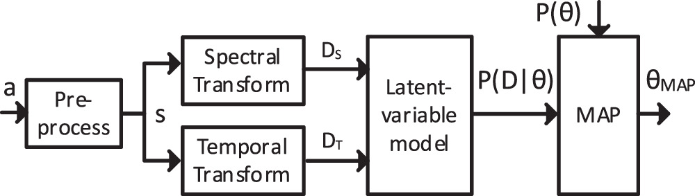
Figure 2. Block diagram of the data processing, with the 3D acceleration signal  the one-dimensional SCG signal
  the spectrally transformed data
  the temporally transformed data
  the likelihood
  the prior
  and the MAP estimation
  .
.
Download figure:
Standard image High-resolution imageNext to the transformations, the SCG signal  is partitioned into segments. A segment is an interval defined by consecutive samples for which
  with
with  defining a threshold (empirically set to 0.06 g), such that large motion artifacts and posture changes are excluded from segments. Heartbeat detection is only performed within segments. In time intervals external to segments, no heartbeat detection is performed, as motion artifacts mask any heartbeats. An example of partitioning into segments may be found in figure 5(a).
The spectral representation  has been introduced in Brüser et al (2013) and comprises local periodicity spectra:

with spectrum  representing local periodicity as a function of
  around a center time
  with
with  = 200 ms. The local periodicity expresses the similarity of two intervals from
  as a function of the period time
  with one interval ranging from
  to
to  and one interval ranging from
  to
to  see figure 3. Due to the prominence of the heartbeats in
  high periodicity typically occurs when
  is equal to the time distance between the last heartbeat before
  and the first heartbeat after
  (which together constitute an IBI). As a typical IBI is much longer than
  multiple spectra will have their peak at the same
  When the periodicity over time is plotted on a gray scale, as is shown in figure 4(c), IBIs will become visible as horizontal bars, with height and duration equal the IBI.
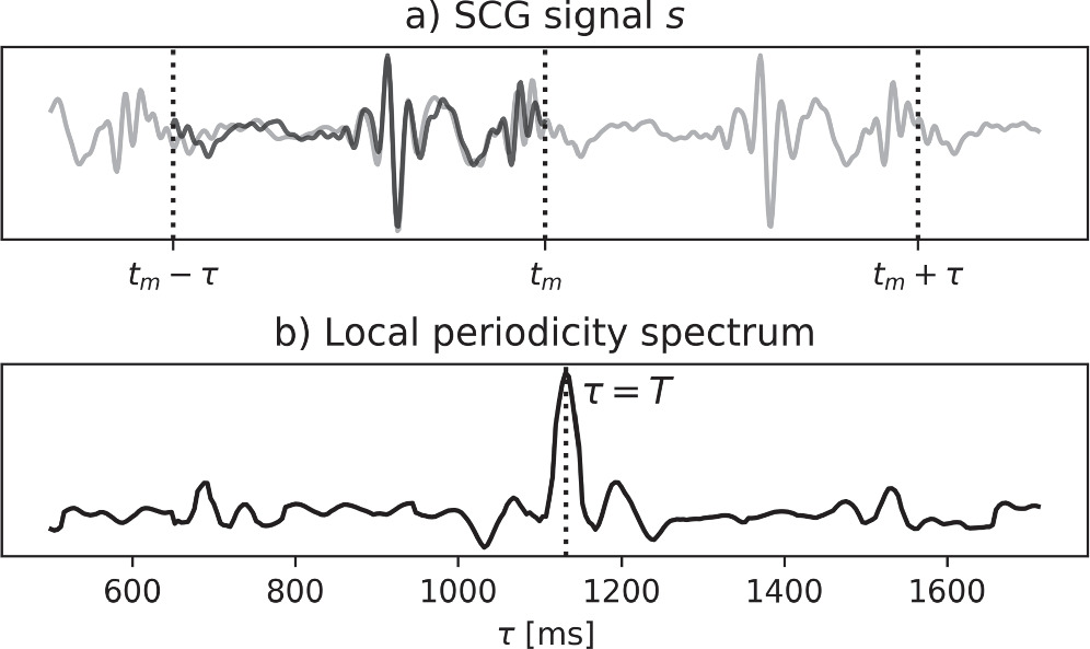
Figure 3. The local periodicity spectrum and how it relates to the SCG signal: (a) the SCG signal  with the interval from
  to
to  overlayed on the interval from
  to
to  (in dark black), and (b) the local periodicity spectrum, with a peak at
  1130 ms, being the time distance between the high-amplitude vibrations (heartbeats) in the first and second intervals.
Download figure:
Standard image High-resolution image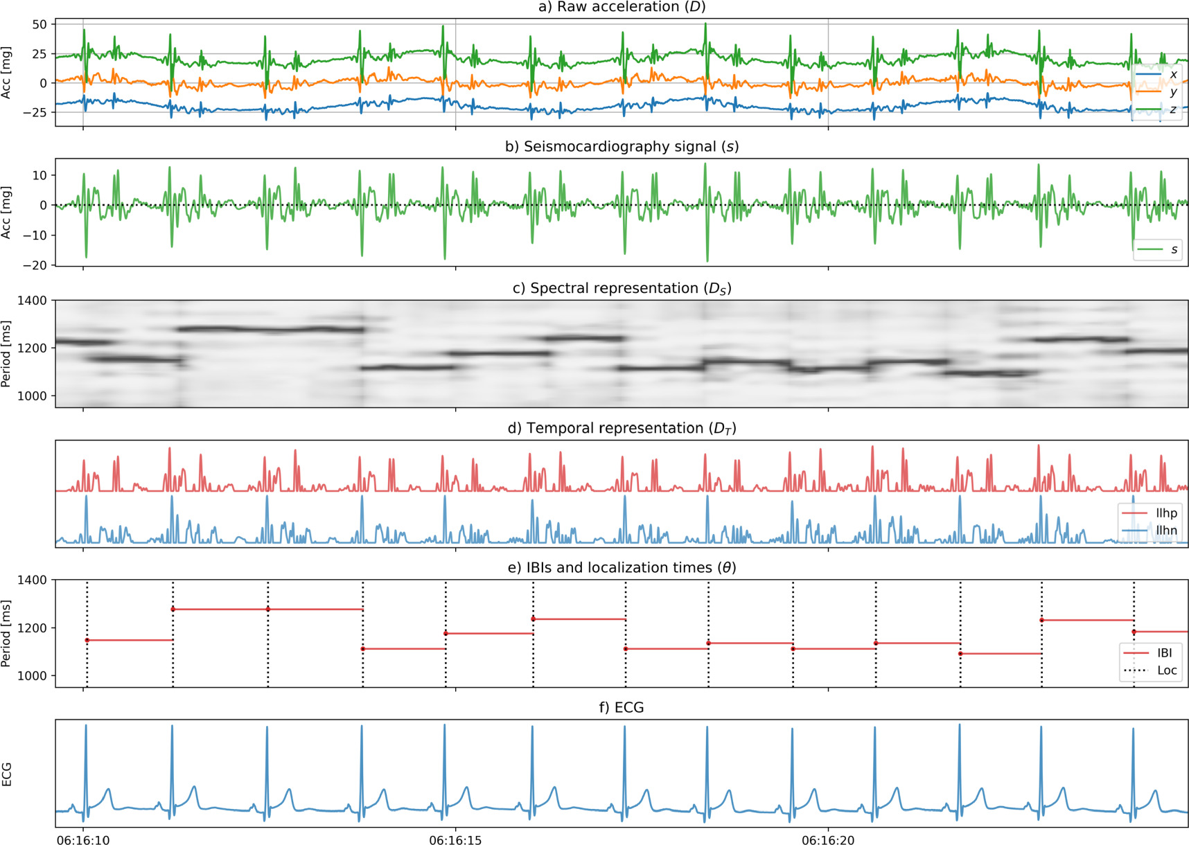
Figure 4. Waveforms for a full example, from top to bottom: (a) the raw acceleration data  (with arbitrary offsets for
 and
and  ), (b) the SCG signal
  (c) the spectral representation
  with higher periodicity in darker shades of grey, (d) the temporal representation
  with the positive and negative components (
 and
and  ), (e) the latent variable
  with the IBIs
  horizontal, at a height equal to the IBI, and the localization times as dashed lines, and (f) the ECG signal.
Download figure:
Standard image High-resolution imageThe temporal representation  expresses the locally normalized magnitude of
  with separate components for the positive and negative parts, see figure 4(d). The normalization for each sample
  is relative to the maximum of the product of the absolute value of
  and a Gaussian window function centered at the sample
  with a standard deviation of 1.7 s (corresponding to an IBI at a heartrate of 35 beats per minute). If we denominate the normalized positive component
  and the normalized negative component
  then we get:

2.3. MAP estimation
Core to our method is a latent-variable model. This describes the stochastic relation between observed data  and
and  and a latent random variable
  ), describing the heartbeats with the starting time
  and the IBIs
  The starting time
  is the localization time of the first beat and the IBIs are equal to the difference between the localization times of beats
  and
and 
 Given knowledge of
  the most probable value of
  can be determined by means of MAP estimation:

which can be rewritten by using Bayes' rule:

with likelihood  and prior
2.3.1. Computing the likelihood
First, we factorize the likelihood per IBI 

with  and
and  the parts of the data in a time interval that is spanned by
  (from
(from  to
to  ). Generally,
  depend on
  iff
iff  However, as the last beat of
  is the same as the first beat of
  the factorization is a (good) approximation. Next, we model the likelihood for each IBI as the product of the spectral likelihood
  and the temporal likelihood

The temporal likelihood is high for data of which the acceleration has a high magnitude at the occurrence of a heartbeat. Therefore, we interpret the locally normalized magnitude (see equation (2)) as the (unnormalized) temporal likelihood:

with  a normalizing constant,
  the localization time of heartbeat
  and
and  either
  or
or  depending on whether we choose to localize beats at the positive or negative component of
  The choice for either
  or
or  will be described in section C3. Figure 4(d) shows temporally transformed data
  of high likelihood, as the peaks in
  coincide with the heartbeats, that are shown as dashed lines in figure 4(e).
The spectral likelihood is high for data of which the spectral peaks match with the IBIs, as is the case in figure 4(c), where the dark horizontal bars (the spectral peaks) match in height and duration with the IBIs in figure 4(e). To compute the spectral likelihood, we define  as a subset of spectra with their center times within the interval spanned by IBI

with  the index of the first spectrum with
  and
and  the index of the last spectrum with
  We interpret the geometric mean of the spectral values in
  as the (unnormalized) spectral likelihood:

with  a normalizing constant.
  will be high if all
  in
in  have a high peak at
2.3.2. Computing the prior
The prior  in equation (4) is computed for each recording individually, by pre-inspecting
  First, for each of the spectra
  the values
  of the highest peaks (
 ) and the period times
  of the highest peaks (
 ) are computed. Next, the period times
  of high peaks (
 with
with  experimentally set to 0.70), are put in a sequence, which is then median filtered (kernel size = 151) to remove outliers. The median-filtered period times,
  are put in a new sequence (at their original positions
  ), and the period times for the positions
  for which no sufficiently strong peak was found (
 ), are linearly interpolated. The resulting sequence
  gives a period time for each time point
  which are used for the computation of the prior. The prior is then computed as follows:

in which each factor  follows a Gaussian distribution with mean
  and standard deviation

The mean  is the geometric mean over the periods
  with
with  from
from  to
to  as in equation (9), and
  is the standard deviation of the period times
2.3.3. Finding the maximum
With (6), (7), and (11), the expression for the MAP estimate  (equation (5)) can be rewritten as follows:

where the expressions for the factors in the right-hand side are given by equations (7), (9), and (11).
As there may be many heartbeats in one recording (typically ~30.000), finding the maximum becomes intractable. Fortunately, the problem can be reformulated into a Markov Decision Process, which breaks down the problem into steps (see supplemental materials). In each step, a current localization time  is advanced to a next localization time
  with
with  by deciding for a value of
  In each step, a reward is obtained, equal to the
  of the corresponding factor in (12):

The value  of a localization time
  is the maximum of the sum of rewards that may be obtained from
  onwards:

which is known as the Bellman equation (Bellman 1952) and provides guidance on decisions for  such that an optimal solution for equation (12) is found. During each step, the process aims to decide for a value of
  that maximizes
  for which it inspects
  IBI candidates, being the
  for the
  highest peaks in
  For each IBI candidate, equation (14) is evaluated recursively, up to a finite horizon, or recursion depth,
  The IBI candidate
  for which
  is maximal is then selected, after which the localization point is advanced to
  until all data have been processed. We chose
  and
and 
The decision process needs a starting point  To this end, the data are partitioned into segments, in which a segment is an interval in which
  with
with  the SCG signal and
  a threshold (empirically set to 0.06 g). We only process segments with a duration
  15 s as in shorter segments the impact of body and sensor settling may be too prominent. For each segment, a starting point
  is searched such that
  is maximal. This is done for both polarities of the SCG signal, so with
  and
and  see (7). The polarity (
 or
or  ) with the highest reward is then chosen and the decision process commences from
  in forward direction as described above, and in reverse direction, in a similar manner, but then with
2.4. Evaluation
2.4.1. Operating point selection
After estimating the IBIs and localization times, the rewards  for each of the beats
  are compared against a threshold
  and beats that have their reward below the threshold are discarded. The thresholding enables the selection of an operating point; decreasing
  decreases the number of detected beats and increases the mean posterior probability of the remaining beats.
2.4.2. Synchronization and pairing with ECG beats
We compute the localization times for the ECG signal, through the detection of R-peaks, using a nonlinear transformation in combination with first-order Gaussian differentiation (Kathirvel et al
2011). The IBIs are then computed as the time-differences between the localization times and IBIs that exceed a threshold  are discarded (we chose
  = 1714 ms, corresponding to 35 beats per minute).
Using the localization times of the SCG and ECG beats, we synchronize the two acquisitions, globally and locally. The global synchronization aims at reducing overall clock offset and drift and was performed by minimizing the localization error between all matched ECG and SCG beats within each recording. An ECG beat and SCG beat become a matched pair if they are each other's nearest neighbors in time, and their distance is less than 250 ms. The localization error, with an example shown in figure 5, may be positive or negative, and may exhibit jumps (caused by changes in the SCG signal morphology) and trends (caused mainly by clock drift). Using a manual procedure, the offset and drift of the SCG signal are adapted such that the localization error trends disappeared, and the mean localization error becomes zero (globally).

Figure 5. Segments and localization errors. (a) The raw acceleration signals for a full recording. The signals are colored within segments and grayed outside of segments. A total of 70 segments is present with a mean duration of 443 s, covering 97.4% of the recording time. (b) The localization errors for synchronization of SCG and ECG over the whole recording (global sync) and over segments (local sync). The markers A and B are timepoints before and after a change in sleeping posture from left to right, and they are detailed further in figure 6(c). The raw acceleration zoomed in around the posture change between A and B (at  03:04:00).
Download figure:
Standard image High-resolution imageIn addition to the global synchronization, we also performed a local optimization aimed at estimating a lower limit for the localization error. For each segment within a recording, the timing offset of the SCG signal is adjusted starting from the global clock offset, until the mean localization error within the segment becomes zero. No drift adjustment is performed for the local synchronization.
2.4.3. Performance metrics and statistics
For performance on beat detection, localization, and IBI estimation, we synchronize over segments without body motion as well as over full recordings. For both cases, we compute the same performance metrics. First, we label all beats; ECG and SCG beats that are in a pair get the label true positive (TP), ECG beats that are not in a pair get the label false negative (FN), and SCG beats that are not in a pair get the label False Positive (FP). From these labels we compute the metrics sensitivity = TP/(TP + FN) and positive predictive value (PPV) = TP/(TP + FP). To get meaningful Sensitivity and PPV metrics, in case of synchronization over segments, we only consider segments with a duration of at least 5 min. In case of synchronization over full recordings, all processed segments are included and the Sensitivity and PPV are computed over the full recording.
For the TP beats, we further define the IBI error as the difference between the SCG and the ECG IBIs and the localization error as the difference between the SCG and ECG localization times. Finally, we perform factor analysis for the RMSE IBI error. For the numeric factors (BMI and Age), we perform Spearman rank correlation, while we perform a Mann–Whitney U test for the categorical factors (Sex and presence of the three most prevalent disorders in the study).
For performance of HR and IHR, we synchronize over full recordings. For the IHR, for both SCG and ECG, a stepwise constant function is computed, with levels equal to the inverse of the IBIs and level changes at the localization times. The two functions are then resampled to 10 Hz, after which the error is computed as the difference between the two, thereby discarding gaps. For the HR, for both SCG and ECG, we take 15 s intervals over which we compute the HR as the inverse of the average of the IBIs, thereby discarding intervals with less than 5 IBIs. The error is then computed as the difference between the SCG and ECG HR.
As our method comprises the extension of an existing method (Brüser et al
2013) with MAP, we also compute the results for the existing method (without MAP). Furthermore, we tune the operating point of the method with MAP, such that its Sensitivity is close to, but not lower than that of the method without MAP. We compute the statistics for both methods and compare them by means of a Wilcoxon signed-rank test. As we have more than one statistic on the same data, we use a Bonferroni-corrected significance level of  (
( 0.001,
  9) to prevent false discoveries.
3. Results
The overnight recordings of 147 participants were preprocessed and segmented, and the median coverage was 79.9% (Q1 = 65.7%, Q3 = 86.2%). This coverage is the combined result of segmentation, with median coverage of 96.6% (Q1 = 94.7%, Q3 = 97.6%), and thresholding within each segment, as described in the section on operating point selection. We obtained performance metrics for the methods with and without MAP, see table 1. All errors were significantly lower with MAP than without. The median RMS IBI error decreased by a factor 2.9 from 25.2 to 8.8 ms (the median IBI was 938 ms). The median RMS localization error decreased by a factor 1.3 from 73.2 to 58.1 ms. Although significant, this reduction factor (1.3) is rather limited when compared to the reduction factor for the RMS IBI error (2.9).
Table 1. IBI, localization and detection results when synchronizing over full recordings, pooled over subjects (N = 147).
| Without MAP | With MAP | |||||||
|---|---|---|---|---|---|---|---|---|
| Median | IQR | 95% intv. | Median | Quantiles | 95% intv. | p | ||
| IBI | ||||||||
| RMSE [ms] | 25.2 | 18.9–38.5 | 11.1–270.2 | 8.8 | 6.5–13.1 | 4.3–68.3 | p < 0.001 | |
| MAE [ms] | 7.4 | 5.9–12.4 | 4.8–116.4 | 4.1 | 3.2–5.5 | 2.3–15.6 | p < 0.001 | |
| Localization | ||||||||
| RMSE [ms] | 73.1 | 58.7–89.0 | 31.1–139.1 | 58.1 | 39.5–80.7 | 18.5–129.0 | p < 0.001 | |
| MAE [ms] | 59.4 | 44.3–74.2 | 21.1–125.5 | 45.9 | 29.0–65.9 | 13.5–115.6 | p < 0.001 | |
| Detection | ||||||||
| PPV [%] | 92.9 | 85.6–97.1 | 69.4–99.3 | 98.0 | 93.5–99.3 | 75.3–99.9 | p < 0.001 | |
| Sensitivity [%] | 76.9 | 67.5–85.1 | 53.7–94.2 | 79.3 | 67.5–86.0 | 34.2–93.2 | — | |
Figure 5 shows how the offset in the localization error can change within one recording and explains the limited decrease of the localization error in case of synchronization over full recordings. Figure 6 shows two short intervals, one from a segment before a posture change and another from a segment after it. In the first segment, the method localized on an earlier positive peak in the SCG signal, while it localized to a later negative peak in the second. The difference in localization caused a change in the offset of the localization error, which could not be compensated for when synchronizing over full recordings. Further examples are given in the supplemental materials.
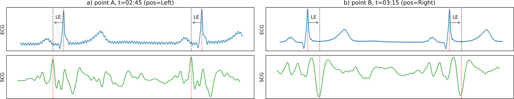
Figure 6. ECG, SCG and beat localizations for timepoints A and B from figure 5, after global synchronization (LE = localization error, pos = sleeping posture). The top graphs show the ECG signal with localized R-peaks. The bottom graphs show the SCG signals with localized heartbeats. The dashed arrows show the localization error. As the morphology of the SCG signal changes, the beat detection algorithm localizes at two different points in the cardiac cycle:at  02:45 it localizes at an early positive peak of the SCG signal, while at
  03:15 it localizes at a later negative peak. As a result, the localization error jumps from negative to positive.
Download figure:
Standard image High-resolution imageWhen synchronizing over segments, on the other hand, the offset in the localization error could be compensated for, and the median RMS localization error decreased from 58.1 ms (as in table 1, with MAP) to 7.90 ms (as in table 2, with MAP). This decrease shows that the higher localization error in table 1 was only due to changes in offset and that the MAP method consistently localizes at the same point (phase) in the cardiac cycle. Again, all errors were significantly lower with MAP than without. The IBI localization error decreased by a factor 2.8 from 15.8 to 5.6 ms, while the RMS localization error decreased by a factor 5.6 from 44.6 to 7.9 ms. As only segments longer than 5 min were included in table 2, the coverage was 77.9% (Q1 = 67.0%, Q3 = 84.9%).
Table 2. IBI, localization and detection results when synchronizing over segments, pooled over segments (N = 3339).
| Without MAP | With MAP | |||||||
|---|---|---|---|---|---|---|---|---|
| Median | IQR | 95% intv. | Median | Quantiles | 95% intv. | p | ||
| IBI | ||||||||
| RMSE [ms] | 15.8 | 8.1–31.0 | 5.0–114.4 | 5.6 | 3.8–9.7 | 2.4–65.6 | p < 0.001 | |
| MAE [ms] | 6.1 | 4.9–9.6 | 4.1–51.1 | 3.5 | 2.7–5.1 | 1.9–21.8 | p < 0.001 | |
| Localization | ||||||||
| RMSE [ms] | 44.6 | 24.8–70.8 | 8.6–132.7 | 7.9 | 4.4–24.6 | 2.7–109.6 | p < 0.001 | |
| MAE [ms] | 30.4 | 11.7–55.5 | 5.7–120.7 | 4.7 | 3.2–11.5 | 2.1–97.4 | p < 0.001 | |
| Detection | ||||||||
| PPV [%] | 98.4 | 91.9–99.7 | 40.3–100.0 | 100.0 | 99.7–100.0 | 41.7–100.0 | p < 0.001 | |
| Sensitivity [%] | 87.4 | 72.7–95.0 | 30.0–99.1 | 88.9 | 76.3–95.2 | 7.4–98.9 | — | |
The IBI error for the method with MAP, when aggregated over all recordings (N = 3.5 × 10⁶ beats), had 95% limits of agreement of −10.6 and 11.1 ms, while the quantiles Q1, Q2, and Q3 were −2.8, 0.0, and 2.8 ms respectively. Mean coverage was 74.6%, over 1236.8 recorded hours.
We investigated the influence of various factors on the performance. The RMS IBI error increased (p < 0.001) due to the presence of sleep disordered breathing (median from 5.2 to 6.2 ms, +19%), movement disorders (median from 5.4 to 6.4 ms, +19%), and sex (median in males 5.4 ms, median in females 5.9 ms, +9%). Furthermore, positive rank correlations for the RMS IBI error (p < 0.001) were found for BMI (0.12) and age (0.22). These numbers relate to the method with MAP in combination with synchronization over segments.
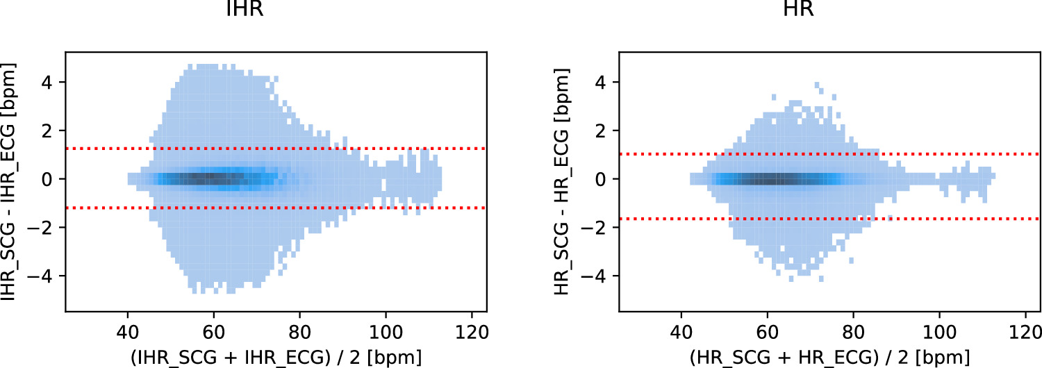
We computed the derived metrics IHR and HR, of which Bland–Altman density plots are shown in figure 7. For the method with MAP, the median error and 95% limits of agreement were 0.00, −1.20 and 1.25 bpm for the IHR and 0.00, −1.65 and 1.03 bpm for the HR. If we define a measurement as being accurate if it is within a range around the reference of either ±5 bpm or ±10% (whichever is larger), then 98.8% of the IHR measurements and 100.0% of the HR measurements were accurate. These percentages were obtained at median coverages of 80.2% and 79.7% respectively (see tables SI and SII of the supplemental materials). The Spearman correlation coefficient was 0.992 for the IHR (p < 0.001) and 0.997 for the HR (p < 0.001). Further metrics and a comparison between the methods with MAP and without MAP may be found in tables SI and SII in the supplemental materials.
Figure 7. Bland–Altman density plots for IHR and HR (method with MAP). The red lines show the 95% limits of agreement. Density cutoff levels are 300 (IHR, N = 4.5 × 10⁶ beats) and 8 (HR, N = 3 × 10⁵ intervals).
Download figure:
Standard image High-resolution image
4. Discussion
We evaluated heartbeat detection from a chest-worn accelerometer in a set of 147 overnight recordings among a diverse population with a variety of sleep disorders. We determined performance for the primary metrics beat detection, beat localization, and IBI estimation, and for the derived metrics HR and IHR. IBI estimation was accurate with an MAE of 3.5 ms, which is less than the sampling period of the SCG signal (4.0 ms) and less than 0.5% of the median IBI time (938 ms). For the derived metrics IHR and HR, we found that 98.8% and 100.0% of all measurements were accurate according to the American National Standard 'Cardiac monitors, heart rate meters, and alarms' (Association for the Advancement of Medical Instrumentation 2002). It should be noted that these percentages were obtained over the covered parts of the recordings (median around 80%).
We have found that adding MAP to the detection method significantly improved the performance. Without reducing sensitivity, the RMS IBI error decreased by a factor 2.8, while the RMS localization error decreased by a factor of 5.6. A possible reason for the improvement is the larger scope of the algorithm; when estimating one IBI (in the Markov Decision Process), all data up to 8 IBIs ahead contribute to the choice for that single IBI.
Table 3 compares our results with other studies on seismocardiography, which reported IBI performance. It should be emphasized that a direct benchmark is not possible, since studies used different protocols, and ultimately, different measuring setups, accelerometers and even performance metrics, so this serves merely as a high-level comparison. Our study shows that it is possible to achieve a high level of accuracy in IBI, HR and IHR estimation also on longer recordings, including changes of posture and body movements, achieving errors at least comparable with the best studies reported even if those were obtained in shorter recordings with subjects laying still in fixed postures (mostly supine).
Table 3. Comparison of results against other studies.
| Year | Study | Sensor | N | Duration | Posture | Results | Method | |
|---|---|---|---|---|---|---|---|---|
| A | 2017 | (Wahlström et al 2017) | Accelerometer | 66 | 1 min | Supine | IBI MAE = 6.10  31.89 ms 31.89 ms | Hidden Markov Model |
| B | 2019 | (Kathirvel et al 2011) | IMU | 25 | 7 min | Supine | HR LoA = −5.06 to 5.66 bpm | Autocorrelated Differential Algorithm |
| C | 2020 | (Cocconcelli et al 2020) | Accelerometer | 20 | 50 min | Supine | IBI RMSE = 4.2 ms | Automatic template calibration and matching |
| 13 | 4 min | Resting in chair | IBI RMSE = 6.2 ms | |||||
| D | 2021 | (Association for the Advancement of Medical Instrumentation 2002) | Gyroscope at head | 19 | 5 min | Supine | HR MAE ≈ 2.5 bpm | Envelope based (Hilbert transform) |
| E | 2021 | (Schipper et al 2021) | Accelerometer | 30 | 40 min | All | HR LoA = −19.3 to 17.8 bpm | Envelope based |
| F | 2023 | (Centracchio et al 2023) | IMU | 21 | 2 min | Supine | LoA = −26.43 to 26.43 ms | Envelope based (Hilbert transform) |
| G | 2023 | This study | Accelerometer | 147 | 8.3 h | All | IBI RMSE = 5.6 ms | |
| IBI MAE = 3.5 ms | ||||||||
| LoA: | ||||||||
| - IBI: −10.6 to 11.1 ms | Maximum A posterior estimation | |||||||
| - HR: −1.6 to 1.0 bpm | ||||||||
| - IHR: −1.2 to 1.3 bpm |
As for the localization error, we found that it was substantially higher when the synchronization was performed over whole recordings (MAE = 45.9 ms, table 1), than over segments without body movements (MAE = 4.7 ms, table 2). The body movements, and perhaps more importantly, posture changes, cause the MAP search algorithm to use different localization points in the cardiac cycle. These cause a change in the offset in the localization error, which is removed by synchronization within a stable posture period. In these intervals, the algorithm consistently assigns localization points to the same point in the cardiac cycle, achieving a relatively small localization error. Note that these intervals were detected by the algorithm itself from the acceleration data, without manual annotations of any kind.
The influence of demographics and sleep disorder prevalence on the performance was limited. Spearman correlation coefficients for age and BMI were only 0.22 and 0.12, while the largest increase in RMS IBI error was due to the occurrence of sleep disordered breathing (from 5.2 to 6.2 ms, +19%), such that still a high level could be maintained. Only a small increase (+9%) in IBI error was found for female over male participants. This shows that the method is robust against body movements and posture changes but also against the presence of sleep disorders and different demographic factors, such as gender.
As stated, the MAP estimation was beneficial for the robustness and accuracy of the method. The probabilistic approach with the latent variable model, Bayes' rule, and the MAP estimation, provided a structured framework for estimation. Separate models could be created for the likelihood and the prior, and the product of the two automatically yielded an objective function. The chain rule of probability allowed for the reformulation of the MAP problem into a Markov Decision Process problem, of which an optimum solution is described by the Bellman equation. The optimum can be approximated by a tree-search algorithm, of which the width and depth can be adjusted to trade accuracy against run time.
A limitation of this study is that subjects with prior diagnosis of cardiac rhythm disorders, most notably atrial fibrillation, were excluded from the study. Especially during sleep monitoring, atrial fibrillation is highly prevalent among patients with sleep-disordered breathing (Linz et al 2022). During cardiac arrhythmias, local periodicity, upon which the method relies, may be absent and therefore results may be worse. Future work should include patients with cardiac arrhythmias and annotation of cardiac rhythms should be made, such that performance under such conditions can be investigated. Another limitation is that the computation of the prior was done by inspection of the full recording; we did not investigate the effect of a constrained look-ahead, which is required for low-latency applications. Furthermore, the Markov Decision Process may be improved; instead of exhaustive search, dynamic programming or reinforcement learning may be applied. Finally, further research may be conducted in the mapping of the three accelerometer axes into the one-dimensional SCG signal. The summation that we used in the present study, reduces sensitivity to changes in the orientation of the sensor with respect to the heart and maintains periodicity, as any linear combination of signals with period T is also periodic with T. However, noise may not be uniformly distributed over the axes, so alternative methods may be evaluated in future work, such as a vector sum which may increase SNR while preserving amplitude periodicity.
The possibility to accurately and robustly estimate HR and IHR, as presented in this paper, together with our earlier published work on respiration (Schipper et al 2021, 2023), may enable cardio-respiratory applications to work with a single sensor. The sensor can be small and only needs mechanical attachment at a single point on the chest, without the need for skin contact. One example of such an application is the detection of patient deterioration using respiration rate and HR (Jacobs et al 2021). Another application may be in positional therapy devices for obstructive sleep apnea, which use a chest worn tactile feedback system to entrain the patient to avoid supine sleeping, thereby reducing the apnea burden (Berry et al 2019). The addition of our method may enable the estimation of residual apnea burden, quantified in the form of the apnea-hypopnea index by using IBIs and respiratory effort from an accelerometer in the therapy device itself (Xie et al 2023).
In conclusion, we propose a method that detects heartbeats from a chest-worn accelerometer, demonstrating robustness and high accuracy during overnight recordings with unrestricted postures and body movements, in a diverse population and in the presence of disorders. This enables applications, that directly measure respiration, to monitor cardiac activity robustly and accurately without the need for an additional sensor.
Acknowledgments
This work has been performed in the IMPULS framework of the Eindhoven MedTech Innovation Center (e/MTIC, incorporating Eindhoven University of Technology, Philips Research, and Sleep Medicine Center Kempenhaeghe). The funders had no role in the study design, decision to publish, or preparation of the manuscript. Fons Schipper, Angela Grassi, Pedro Fonseca, and Jan Brouwer are employed by Philips Research. The employer had no influence on the study and on the decision to publish. Ruud van Sloun is employed by both Philips Research and by the Eindhoven University of Technology. The other authors declare no competing interests.
The authors would like to thank Stan Hullegie, Bertram Hoondert (Kempenhaeghe), Ad Rommers, and Henry van Vugt (Philips) for their help in data acquisition.
Data availability statement
The data cannot be made publicly available upon publication because they are owned by a third party and the terms of use prevent public distribution.
Supplementary materials (1 MB DOCX)