

Abstract
Gradient and spin echo (GRASE) is widely employed in arterial spin labeling (ASL) as an efficient readout sequence. Hemodynamic parameter mappings of perfusion, such as cerebral blood flow (CBF) and arterial transit time (ATT), can be derived via multi-delay ASL acquisitions. Multi-delay ASL perfusion imaging inevitably suffers limited signal-to-noise ratio (SNR) since a motion-sensitized vessel suppressing module has to be employed to highlight perfusion signals. The present work reveals that in multi-delay ASL, manipulation of GRASE sequence on either planar imaging echo echo train for adjusted spatial resolutions or FSE echo train for modulated extent of T2-blurring can significantly alter the mapping contrasts among tissues and among cerebral lobes under different pathways of blood circulation, and meanwhile regulates SNR. Four separate multi-delay ASL scans with different echo train designs in 3D whole brain covering GRASE were carried out for healthy subjects to evaluate the variations in regard to the parameter quantifications and SNR. Based on the quantification mappings, the GRASE acquisition with moderate spatial resolution (3.5 × 3.5 × 4 mm3) and segmented kz scheme was recognized for the first time to be recommended for more unambiguous CBF and ATT contrasts between GM and WM in conjunction with more enhanced ATT contrast between anterior and posterior cerebral circulations, with reasonably good SNR. The technical proposal is of great value for the cutting-edge research of a variety of neurological diseases of global concerns.
Export citation and abstract BibTeX RIS
Introduction
Arterial spin labeling (ASL) (Detre et al 1992) is an advanced MRI technique in measuring arterial blood perfusion and has been widely applied in clinical examinations and research of the human brain (Telischak et al 2015, Haller et al 2016). With the advantage of labeling protons in blood using radiofrequency pulses rather than introducing exogenous contrast agents, this technique has found its great benefit as a routine scan for examinations of a wide variety of diseases in the brain (Grade et al 2015). The pseudo-continuous ASL (pCASL) technique has been recommended for labeling preparation owing to its high inversion efficiency for high SNR in the perfusion-weighted imaging (PWI) (Dai et al 2008, Alsop et al 2015). Gradient and spin echo (GRASE) (Oshio and Feinberg 1991), as a combination of fast spin echo (FSE) and echo planar imaging (EPI), is commonly exploited as the acquisition sequence for ASL applications due to its rapid sampling efficiency and high view-ordering flexibility (Feinberg et al 1995). Although GRASE requires elaborate phase corrections and echo time shifting for EPI bipolar gradients as well as phase stability along the FSE echo train, the employment of GRASE bears considerable benefits, such as less susceptibility to B0 inhomogeneity owing to the FSE refocusing mechanism, as well as speedy acquisition defined by the EPI factor and echo train length (ETL) of the FSE train.
Multi-delay ASL has been applied to human brain examinations and research for quantifications of perfusion hemodynamic parameters (Dai et al 2012, Wang et al 2013, 2014). Without the invasive introduction of contrast agents, hemodynamic parameters, such as cerebral blood flow (CBF), arterial transit time (ATT), and arterial cerebral blood volume (aCBV), can be conveniently estimated (Wang et al 2013). Quite a few factors could influence the accuracy of the parameter quantifications. Recent studies have primarily focused on settings of post-labeling delays (PLDs), and reported that the factors including the number of PLDs, separations between PLDs, and the covered range are important for quantifications (Qiu et al 2012, Mezue et al 2014, Wang et al 2014). Even though 3D GRASE has been commonly used as the readout sequence for multi-delay ASL (Fernandez-Seara et al 2005, 2008; Gunther et al 2005), the influence of various designs of the sequence on the parameter quantifications has not been explicitly investigated. The manipulation of GRASE sequence allows adjustment of EPI factor, number of FSE segments, and 3D k-space segmentation along alternative phase-encoding dimensions. These variations in the sequence directly dictate echo-train duration (ETD) and in-plane spatial resolution, both of which may induce quantification variations in mapping the hemodynamic parameters so that in-depth investigation is demanded imperatively. Besides, a motion-sensitized module for vessel signal suppression is usually set prior to the acquisition (Balu et al 2011, Dai et al 2012, Qin et al 2014), which is detrimental for signal-to-noise ratios (SNRs) of the hemodynamic parameter mappings as the SNR of originally acquired perfusion signals can be largely diminished. Because of this, acquisition of multi-delay ASL requires sufficient SNR in the PWI. Therefore, SNR needs to be assessed along with the quantifications while manipulating GRASE for varied spatial resolutions.
In this study, the influence of a couple of important designs of a whole brain-covering GRASE sequence on the CBF and ATT mappings of multi-delay ASL was demonstrated for a group of healthy volunteers. Specifically, with a suitable EPI factor for moderate in-plane spatial resolution (voxel size: 3.5 × 3.5 × 4 mm3) and a split of FSE echo train for segmented kz acquisition, sharper gray matter (GM)/white matter (WM) contrast in both CBF and ATT maps together with greater distinction reflecting anterior and posterior circulations in ATT maps could be simultaneously achieved. Meanwhile, reasonably good SNRs for both mappings were maintained. This customized configuration is proposed for clinical examinations.
Materials and methods
Separate off-resonance and T2 (SORT) view-ordering strategy (Mugler 1999) was applied in the 3D GRASE sequence, as demonstrated in figure 1. GRASE is one of the fastest readout sequences by combining the speed benefits of EPI and FSE (figure 1(a)). For the SORT, the basic idea is to arrange echo signals from EPI and FSE echo trains respectively to different phase-encoding dimensions (i.e. ky and kz). k-space lines from each EPI echo train of GRASE are arranged along ky (figure 1(b)). In the present design, three GRASE shots were utilized to complete each 2D kx–ky partition in an interleaved fashion. In other words, all echo signals from each FSE refocusing segment were bundled to fill the k-space lines in correspond to a single kz (in head-foot, or slice direction) partition. Bundles of echo signals from different FSE segments were respectively filled in a center-out way along kz (figure 1(c)). Therefore, if a scanning protocol should be without slice oversampling and kz partial Fourier settings, the number of FSE segments would be set exactly equal to the number of slice (or equivalently say, kz). Notably, a segmented interleaved kz acquisition could be applied by cutting the FSE echo train in half in each GRASE shot and repeating all previously performed acquisition once again with a different set of shifted slice (i.e. kz) phase-encodings, although the scan duration was doubled with this segmented kz design.
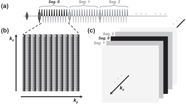
Figure 1. Schematic 3D GRASE sequence with SORT view-ordering design (a) a GRASE sequence is comprised of EPI trains inserted into FSE focusing segments (only the first three refocusing segments, segs. 0, 1, and 2, are displayed for simplicity). Gradient blocks other than the EPI bipolar trains are omitted in this illustration. (b) The kx–ky partition of a 3D k-space. The EPI echo lines are filled in this partition in an interleaved fashion. The solid arrow lines signify the sampled k-space lines from the above EPI echo train. The dash lines are to be filled with the same segments from subsequent GRASE shots. (c) Each FSE refocusing segment is responsible for a partition at different kz, and all the segments are arranged in a center-out fashion along kz for k-space filling.
Download figure:
Standard image High-resolution imageFor demonstration, the neatly designed 3D GRASE preceded with the pCASL preparation module, background suppression composite pulses, and the vessel suppression module was performed with a healthy 29 y/o male as a representative of four recruited volunteers (3 males and 1 female, 33.25 ± 7.18 y/o) under United Imaging Healthcare review board at 3.0 T using a uMR 790 scanner (Shanghai United Imaging Healthcare, Shanghai, People's Republic of China). All the volunteers passed the routine MRI safety screening and gave signed informed consent (reference number: 0000630). Sequential multi-delay ASL acquisition with PLDs of 500, 1000, 1500, 2000, and 2500 ms and averaging number of two for ASL labeling and control acquisitions in each PLD was exploited for quantifications of the brain perfusion hemodynamic maps. Proton density-weighted M0 for calibration was scanned once. The T2 preparation motion-sensitized module with a specific velocity encoding (VENC) was utilized immediately before GRASE readout for vessel signal suppression. Two in-plane matrix sizes of 64 × 64 and 80 × 80 were collected with EPI factors of 21 and 25, respectively. Field-of-views (FOVs) of 224 × 224 and 192 × 192 mm2 were set respectively for these two matrix sizes, which resulted in in-plane resolutions of 3.5 × 3.5 mm2 (regular resolution, denoted as RR) and 2.4 × 2.4 mm2 (high resolution, denoted as HR). Slice oversampling rate was set to 10% and ¾ partial Fourier along kz was used. 4 mm thickness × 32 axial slices were collected. For each resolution configuration, FSE echo train length (ETL) of 27 and 13 were applied in correspond to conjoint kz (i.e. one kz segment, denoted as S1) and segmented kz (i.e. two kz segments, denoted as S2) traversing designs, respectively. Therefore, in total the alternative settings of both EPI factor and FSE ETL constituted four types of GRASE acquisitions as illustrated in figure 2. For simplicity, the notations of RR-S1, RR-S2, HR-S1, and HR-S2 were used respectively to represent these acquisitions or datasets. Bandwidth was 2600 Hz/pixel. TR/TE settings were 6100/13.86 ms and 6200/17.02 ms for the regular resolution and the high resolution sequences, respectively. Each proton density-weighted M0 was scanned with the same parameter settings as its corresponding control/label pair, however without the magnetization preparation modules. The scanning durations were 6:26, 12:46, 6:33, and 12:58 min, respectively. Image interpolation rate of two was applied in the image domains for the four datasets. Thus, the nominal in-plane resolutions in all pristine and processed images were actually doubled (1.75 × 1.75 and 1.2 × 1.2 mm2 for RR and HR, respectively). The major scanning parameters are summarized in table 1.

Figure 2. Four illustrative shots of the proposed GRASE acquisition designs. Gradient blocks other than the EPI bipolar trains are omitted in this illustration for simplicity. 21-EPI echo train (blue blocks) design for regular spatial resolution GRASE sequences with conjoint kz acquisition, RR-S1 (a) and with segmented kz acquisition, RR-S2 (b). 25-EPI echo train (red blocks) design for high spatial resolution GRASE sequences with conjoint kz acquisition, HR-S1 (c) and with segmented kz acquisition, HR-S2 (d).
Download figure:
Standard image High-resolution imageTable 1. Scanning parameters for the four GRASE acquisitions employed in the study. ETL = echo train length of FSE, ETD = echo train duration of GRASE.
| Voxel size (mm3) | EPI factor | ETL | ETD (ms) | TE (ms) | TR (ms) | |
|---|---|---|---|---|---|---|
| RR-S1 | 3.5 × 3.5 × 4.0 | 21 | 27 | 385 | 13.86 | 6100 |
| RR-S2 | 13 | 191 | ||||
| HR-S1 | 2.4 × 2.4 × 4.0 | 25 | 27 | 472 | 17.02 | 6200 |
| HR-S2 | 13 | 234 |
For anatomical images as the mapping reference, a T1 FSE fluid-attenuated inversion recovery (FLAIR) sequence was scanned with the same center of FOV, through-plane FOV, slice number, and slice thickness as the ASL scans. TR/TE were 2720 and 10.24 ms. In-plane FOV was 230 × 200 mm2 and matrix sizes were 352 and 306, respectively. Phase-encoding direction was set in left to right. Bandwidth of 180 Hz/pixel was applied. The scan was accelerated with uCS technology developed by United Imaging Healthcare, based on the compressed sensing theory (Lustig et al 2007, 2008). The scanning duration was 2:11 min. For all ASL and the anatomical scans, a 32-channel head coil was used.
The pristine control and tag images of multi-delay ASL were fitted to the general kinetic model based on the well-mixed single-compartment theories (Buxton et al 1998) for quantifications of perfusion hemodynamic parameters. With computational prerequisites including scanning parameters, physical and physiological constants, and high spatial resolution T1 FSE FLAIR anatomical images, the computation was carried out using Bayesian Inference for arterial spin labeling MRI (BASIL) toolset incorporated in FMRIB software library (FSL) image analysis and statistical tools (Chappell et al 2008, 2010). In the course of the processing, the ASL images and the parameter mappings were co-registered against the T1 FSE FLAIR images and skull-stripped. The general kinetic model for pCASL is mathematically described by
where ΔM(t) is the difference magnetization between control and label conditions as a function of time t, M0b is the equilibrium magnetization of arterial blood to be labeled and is the quantity equivalently measured by the separate acquisition of proton density-weighted M0, f is CBF, Δt is ATT, τ is labeling duration, T1b is the T1 relaxation value of the arterial blood, and T1app is the apparent T1 relaxation value of the tissue and is expressed as

where T1 is the relaxation value of the tissue of interest and λ is brain-blood partition coefficient. CBF and ATT maps were estimated in the final output after a multi-parametric Bayesian fitting process based on the theoretical model. GM/WM segmentation was also performed, by which the average CBF and ATT were calculated for each type of segmented tissue.
Results
Each of the four volunteers underwent scans with four different acquisitions such that 16 datasets in total were collected. Figure 3 shows the CBF maps from the four data acquisitions for the 29 y/o male volunteer. 15 equidistant slices out of the full brain covering 32 slices are displayed as a representation. For the data with the regular resolution, the CBF maps with segmented kz acquisition (RR-S2, figure 3(b)) show more prominent GM/WM contrast in comparison to those with conjoint kz acquisition (RR-S1, figure 3(a)). Similarly, as comparing HR-S2 (figure 3(d)) and HR-S1 (figure 3(c)), this sharper GM/WM contrast can also be observed at a higher spatial resolution, although the high resolution maps (figures 3(c) and (d)) suffer relatively lower SNR. Regardless of whether or not the kz segmentation is employed, the low SNR in the high resolution images is a considerable issue and will be noted in the discussion section.
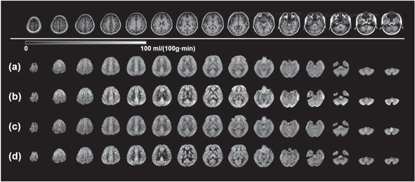
Figure 3. CBF maps of multi-delay ASL using four GRASE acquisition designs. The mapping results were acquired on a 29 y/o subject as a representation. 15 equidistant CBF maps out of total 32 slices are shown as a representation. Top row: T1 FSE FLAIR anatomical images for the same corresponding slices. With RR-S1(a), RR-S2(b), HR-S1(c), and HR-S2(d) acquisitions, variations of the CBF maps were resulted.
Download figure:
Standard image High-resolution imageThe ATT maps from the four datasets on the volunteer are shown in figure 4 for the same 15 slices as in figure 3. Similarly as what has been found in the CBF maps, not surprisingly, the regular spatial resolution ATT maps (figures 4(a) and (b)) present higher SNR than those with the high resolution (figures 4(c) and (d)). Notably however, this SNR loss is more significant compared to that of the CBF maps. The most remarkable difference in comparing these four sets of maps is that the ATT contrast among particular regions of the brain is much more pronounced in the GRASE acquisition with regular resolution and segmented kz (RR-S2, figure 4(b)). The contrast is interpreted in two perspectives. First if we look at tissues, WM generally exhibits longer ATT than GM. Second, occipital lobe and cerebellum in posterior circulation show longer ATT than frontal, parietal and temporal lobes in anterior circulation. This distinct contrast becomes obscure when utilizing conjoint kz GRASE acquisition (figure 4(a)). When high resolution acquisition is employed, SNR becomes an issue and this distinct contrast fades away (figure 4(d)). Further, if conjoint kz is used for the high resolution acquisition, an even more depressed contrast in obscure appearance is resulted (figure 4(c)).
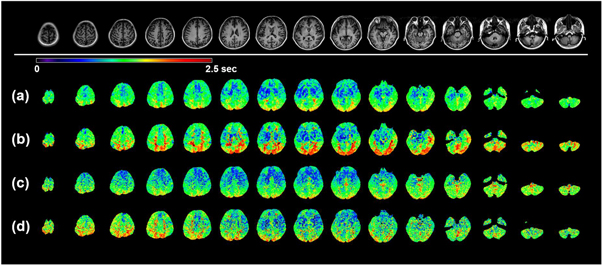
Figure 4. ATT maps of multi-delay ASL using four GRASE acquisitions. The mapping results were acquired on the 29 y/o subject as a representation. 15 equidistant ATT maps out of total 32 slices are shown as a representation. Top row: T1 FSE FLAIR anatomical images for the same corresponding slices. With RR-S1(a), RR-S2(b), HR-S1(c), and HR-S2(d) acquisitions, variations of the ATT maps were resulted.
Download figure:
Standard image High-resolution imageTwo representative slices are selected from figures 3 and 4, and are displayed head-to-head in figure 5. In this enlarged comparison, the mapping characteristics mentioned above can be more clearly recognized. As for the CBF maps (figures 5(a) and (c)), high resolution kz segmented acquisition (HR-S2) offers the greatest GM/WM contrast in spite of the compromise of SNR. Nevertheless, RR-S2 shows reasonably good GM/WM contrast with the highest confidence in regard to SNR. The ATT maps for the four acquisitions are displayed in figures 5(b) and (d). Both regular and high resolution segmented kz acquisitions (RR-S2 and HR-S2) provide greater contrast in ATT maps compared to their counterparts using conjoint kz acquisitions (RR-S1 and HR-S1). However, diminished SNR is inherited for HR-S2. It is obvious that the occipital regions merely show a mosaic of moderately long and long ATT spots, indicative of insufficient SNR in the ATT estimation. An advantage of the regular resolution ATT mapping over the high resolution is that for GM abundant regions, such as the basal ganglia, clearer morphologies emerge (figure 5(d)), suggesting that the transit time contrast under the scanning parameters is superior. The morphological characteristics appear as well for the CBF mapping as presented in figures 5(a) and (c).

Figure 5. CBF and ATT maps of two exemplary slices magnified from figures 3 and 4. Left column: anatomical images of T1 FSE FLAIR for the two slices. Four GRASE acquisitions RR-S1, RR-S2, HR-S1, and HR-S2 are arranged from left to right for the CBF maps for the first slice (a) and second slice (c) and the ATT maps for the first slice (b) and second slice (d).
Download figure:
Standard image High-resolution imageThe CBF and ATT contrast differentiation among different acquisition approaches can be more clearly exhibited in the coronal and sagittal views. In figure 6, the coronal and sagittal central slices of the 3D brain of the volunteer for both CBF and ATT maps are shown. The enhanced GM/WM contrast in CBF maps and circulation contrast in ATT maps are evidently discerned in figures 6(b) and (d) using segmented kz acquisition in comparison to those using conjoint acquisition (figures 6(a) and (c)). Meanwhile, figures 6(b) and (d) display reduced degree of blurring along slice direction in respective comparison to figures 6(a) and (c), especially evident in the CBF mappings. In addition, similarly to what has been shown in axial slices in figures 4 and 5, in ATT maps of figure 6(b) the prolonged blood transit times in the occipital lobe and cerebellum in posterior circulation in contrast to frontal, parietal and temporal lobes in anterior circulation are clearly identified.

Figure 6. CBF and ATT maps in coronal and sagittal views using four GRASE acquisitions. The mapping results were acquired on the 29 y/o subject as a representation. Left two and right two columns are CBF maps and ATT maps, respectively. The results by four GRASE acquisitions RR-S1, RR-S2, HR-S1, and HR-S2 are respectively shown in (a), (b), (c), and (d).
Download figure:
Standard image High-resolution imageThe four acquisition scans were conducted on each one of the four healthy volunteers and 16 datasets in total were collected for analysis. GM/WM tissue segmentation is performed in the BASIL toolset, based on which the CBF and ATT average values for the two tissues can be separately obtained. For the four acquisitions, these values are then averaged again over the four subjects and summarized in table 2 for comparison. The CBF of GM is consistently higher than that of WM in each acquisition. Nonetheless, among the four acquisitions for the two tissues, there are substantial variations with the greatest discrimination of about 11 ml/(100 g·min). As can be directly observed in the CBF maps and the table, greater GM/WM contrast emerges when segmented kz acquisitions (RR-S2 and HR-S2) are employed. In other words, if kz is conjointly acquired (RR-S1 and HR-S1), the GM/WM CBF contrast becomes insignificant. If we compare the two resolution acquisitions (RR and HR) with the same kz acquisition strategy (S1 or S2), the absolute GM/WM CBF values and their contrasts are virtually equivalent. As for the ATT statistics for these four acquisitions, WM generally shows slightly longer ATT than GM with an exception by using RR-S1. The segmented kz acquisition in the regular resolution (RR-S2) gives rise to the most distinct GM/WM contrast. Not quite distinguishable ATT values between GM and WM are estimated using other acquisitions.
Table 2. Summary of average CBF and ATT for GM and WM over the four subjects using the employed four GRASE acquisitions.
| CBF (ml/(100 g·min)) | ATT (ms) | |||
|---|---|---|---|---|
| GM | WM | GM | WM | |
| RR-S1 | 51.92 | 38.42 | 1194 | 1183 |
| RR-S2 | 57.97 | 31.03 | 1270 | 1388 |
| HR-S1 | 50.53 | 37.66 | 1263 | 1278 |
| HR-S2 | 55.96 | 27.96 | 1350 | 1375 |
In conjunction with standard deviations determined among different subjects, the CBF and ATT statistics from table 2 were separately converted into column charts for convenient comparison, as shown in figure 7. The quantification variations in the average CBF and ATT among examined subjects are readily identified this way. It is straightforward in the charts to visualize that RR-S2 and HR-S2 give rise to the more conspicuous GM/WM contrast in CBF maps; and RR-S2 brings up the greatest GM/WM ATT contrast. At the other end, the HR-S1 design yields the least distinct contrast in CBF, closely followed by RR-S1. RR-S1 even gives unreasonable relative ATT values for GM and WM.

Figure 7. Comparisons of average CBF and ATT for GM and WM for the four GRASE acquisitions. The average CBF and ATT values are from table 2. Standard deviations were calculated based on subject to subject variations.
Download figure:
Standard image High-resolution imageDiscussion
Four different GRASE sequence designs were investigated for quantifications of perfusion hemodynamic parameters in the human brain. High resolution acquisitions can intuitionally promote the diagnostic inspection on microstructure perfusion with the benefit of elimination of partial volume effects, but inherently low SNR can be detrimental to the parameter mappings. Since the T2 preparation motion-sensitized module must be applied prior to GRASE sequence for vessel signal suppression, the significant loss of SNR attributed to the use of the module cannot be avoided. Because a long PLD (∼1500 ms or longer) is usually exploited in single-delay ASL, negligible vessel signals remain in the perfusion images. Thus, the use of the vessel suppression module in single-delay ASL is unnecessary so that this limited SNR is an exclusive issue for multi-delay ASL. On the other hand, a GRASE shot can be quite long (a few hundred ms) in view of the incorporation of a series of EPI echo trains into an FSE sequence. For the SORT view-ordering in GRASE, if a long FSE train is not split up for segmented kz acquisition, more severe exponential T2-decay occurs in the course of the shot, inevitably producing blurring (Zhou et al 1993) along slice direction in the 3D image. kz segmented acquisition makes the GRASE shot shorter and thus should be favorable for more unbiased quantifications of hemodynamic parameters by multi-delay ASL. As listed in table 1, ETD of segmented kz acquisition is about half of that of conjoint kz acquisition upon using the same EPI factor (191 versus 385 ms and 234 versus 472 ms).
The four different GRASE designs were applied to a group of subjects and quite consistent results were acquired such that the quantifications of the hemodynamic perfusion parameters possess statistical significance. For the comparison of the quantitative CBF mapping, the observations can be interpreted as below.
RR-S2 (figure 3(b)) and HR-S2 (figure 3(d)) show more striking perfusion contrast between GM and WM as opposed to RR-S1 (figure 3(a)) and HR-S1 (figure 3(c)), owing to mitigated T2-decay induced image blurring while using segmented acquisitions. Specifically, HR-S2 exhibits the most distinct GM/WM CBF contrast, closely trailed by RR-S2. This contrast is obscure for RR-S1 and HR-S1, based on which we verify that the longer the echo train, the blurrier the contrast, in analogy to the well-recognized fact of T2-blurring of image. This blurring in contrast (as in figure 6) is likely caused by the blurring effects of pristine images across slices due to long FSE segments in direct association with the number of slice phase-encodings based on the SORT design. Therefore, in addition, it can be determined that the degree of blurring in the contrast has a direct relationship with ETD as listed in table 1 for the four acquisitions.
RR-S2 (figure 3(b)) offers higher SNR than HR-S2 (figure 3(d)), as well as more indiscrete morphologies of anatomical structures, such as basal ganglia. A moderate in-plane resolution (3.5 × 3.5 mm2) with the EPI factor setting of 21 in the present study should be favored for great certainty in estimating CBF. This observation suggests that CBF can be an inherently low spatial resolution quantity determined by multi-delay ASL.
Quite a lot of factors may influence the accuracy of CBF quantification, nonetheless the accuracy of the obtained absolute CBF is beyond the scope of the present study. But it would be of interest to compare with previous ASL studies with perfusion quantification information. In the early years of multi-delay pCASL, a so-far highly-cited study by Dai et al (2012) reported average CBF values of GM and WM by spiral acquisitions for a group of young adults, despite that a much simplified quantification algorithm was employed. An average GM CBF of ∼60 ml/(100 g·min) was obtained in their study. By RR-S2 in the present work, the average CBF value of GM agrees quite well with that. However, the estimated average CBF of WM using RR-S2 deviates from the reported value at about 20 ml/(100 g·min). Nevertheless, HR-S2 produces an average WM CBF value in better agreement with what was reported. If it is not brain perfusion characteristics of the examined subjects, the deviation can be attributed to residual T2-blurring of GRASE, segmentation errors for GM and WM profiles and percentages for partial volume effects, or the use of oversimplified estimation algorithms in the previous study.
ATT mapping reflects arrival times of labeled spins to voxels of tissues, which should be of critical importance to examine perfusion hemodynamics. Different acquisition strategies provide varied ATT maps for the four subjects, which can be interpreted in a few perspectives as follows.
Similarly to the CBF characteristics, RR-S2 (figure 4(b)) and HR-S2 (figure 4(d)) yield greater tissue contrast in respective comparison to RR-S1 (figure 4(a)) and HR-S1 (figure 4(c)). Amongst the four acquisitions, RR-S2 shows the greatest GM/WM tissue contrast (as summarized in table 2 and figure 7) and well depicts the contrast between cerebral lobes under different pathways of anterior and posterior circulations (highlighted prolonged arrival times in occipital lobe and cerebellum as in figures 4–6). RR-S1, HR-S1, and HR-S2 are likely to provide less reliable ATT quantification as they don't differentiate GM/WM tissues and circulations well enough. Specifically, with RR-S1, the average GM ATT is counterintuitively longer than that of WM, thus may not be considered appropriate for multi-delay ASL acquisition. It is a remarkable finding that scanning parameters of GRASE utilized in RR-S2 are more advantageous for ATT mapping.
Other than the tissue and circulation contrasts, the RR acquisition sets (figures 4(a) and (b)) generally show higher SNR than the HR ones (figures 4(c) and (d)). Similarly as in the CBF mappings, the regular resolution acquisition outperforms the high resolution as well for ATT estimation. The primary reason for this SNR difference is that RR possesses larger voxel size in the pristine ASL control/label images than HR does, such that this higher sensitivity passes on to the ATT determination from the perfusion curve. This finding is in line with the study by Dai et al (2012) who found that transit delay is an inherently low spatial resolution quantity.
Again, it is not within the scope of the present study to determine the quantification accuracy of ATT maps. But we believe that making comparisons with previous studies could be appealing to a broad range of scientific readers. In the same report by Dai et al, average GM and WM ATTs were determined for the young adults as 1.41 ± 0.18 and 1.56 ± 0.09 s, respectively. In table 2, the obtained average ATT GM/WM contrast over investigated subjects by RR-S2 agrees well with the contrast posed by the reported values. The 29 y/o representative volunteer has GM ATT of 1.35 s and WM ATT of 1.48 s, which perfectly fall within the reported value ranges. HR-S2 can also give reasonable estimate for GM, but not for WM presumably due to limited SNR for WM abundant regions. Similarly to CBF estimation, S1 acquisition sets provide ATTs far off the ranges. Longer ETDs in S1 sets introduce a certain degree of blurring in the pristine ASL images, and the impact can be carried over to the perfusion curve as a function of PLD in the fitting for ATT estimation, bringing about unreasonable ATT values for tissues. It is suggested that one should beware of the ETD of GRASE while conducting multi-delay ASL scans.
The limitation of the recommended GRASE design is that the scanning duration is a bit long with five PLDs. Elaboration of variable flip-angle strategy (Hennig et al 2004, Liang et al 2014, Kemper et al 2016) could find its benefit to be applied in the conjoint kz acquisition of GRASE for shorter scanning time. Future directions on sequence acceleration, such as parallel imaging approaches including controlled aliasing in parallel imaging results in higher acceleration (CAIPIRINHA) (Breuer et al 2005, 2006), should be of imperative demand for widespread adoption of the proposed acquisition scheme in clinical applications.
Conclusions
In summary, in this work, by manipulating GRASE acquisition in multi-delay ASL sequence with dual EPI factors for a switch for spatial resolution and dual FSE train lengths for T2-blurring modulation, the ATT and CBF mappings for a group of subjects were obtained and analyzed. Among the four acquisition designs, regular resolution with segmented kz acquisition (RR-S2) balances well between SNR and contrasts, as can be clearly revealed in both CBF and ATT mappings. This customized GRASE sequence incorporated in multi-delay ASL has great potential to reasonably reflect brain perfusion hemodynamics and thus is proposed for more distinct tissue and perfusion circulation contrasts. Most importantly, the investigation contains scientific significance for accurate and precise quantifications and amplified mapping contrasts of the important physiological parameters associated with blood perfusion in the human brain and thus is of great value for the cutting-edge research of a variety of neurological diseases of global concerns.
Acknowledgments
The authors would like to thank Dr. Qiang "Al" Zhang†, Dr. Weiguo Zhang‡, Dr. Guosheng Steve Tan†, Dr. Guobin Li†, Dr. Qun Chen†, and Dr. Hongdi Li‡ (†Shanghai United Imaging Healthcare Co., Ltd., Shanghai, People's Republic of China; ‡UIH America, Inc., Houston, TX, United States of America) for the support to realize the work.
This work was presented in part at the 31st Annual Meeting of the ISMRM in May 2022 (Abstract No. 4881).
Conflict of interest
The first and last authors are employees of UIH America, Inc., Houston, TX, United States of America. Other authors are employees of Shanghai United Imaging Healthcare, Co., Ltd., Shanghai, People's Republic of China.
Appendix.: Additional results
Appendix. Measurements of pSNR and pSNR efficiency
To further compare the performance of the four GRASE designs quantitatively, we conducted SNR analysis. The computed CBF and ATT maps may inevitably exhibit relatively large variations in image background outside of an imaging subject, and are usually processed with a template of human brain mask. Nonetheless, SNRs of the perfusion-weighted images obtained immediately after control/label subtraction at the employed PLDs directly dictate the SNRs of the hemodynamic parameter maps, thus can be utilized as an indirect quantitative measure of sensitivity for the hemodynamic parameter maps. Perfusion signal-to-noise ratios (pSNRs, defined as perfusion signals/noise) of perfusion-weighted images can be quantified conveniently. Here, with two averages at a single PLD of 1500 ms from the same multi-delay datasets in this study, the perfusion of the superior slice from figure 5 was taken as a representation to quantify the pSNR among the four GRASE acquisitions, as shown in figure A1. Regional perfusion intensities were measured by selecting three regions of interest (ROIs) in the lateral and posterior regions of the brain. A region of background noise with virtually the same area in the posterior region was circled for the pSNR comparison.

Figure A1. Comparison of pSNRs in perfusion-weighted images for the four GRASE acquisitions. The representative perfusion images (a)–(d) of a superior slice are from the same datasets RR-S1, RR-S2, HR-S1, and HR-S2, respectively, in this study. They were acquired with two averages at a single PLD of 1500 ms. The statistical results of the voxels are shown on the side of each ROI.
Download figure:
Standard image High-resolution imageBesides the pSNRs, we also calculated pSNR efficiency defined as  where t is the scanning duration of the multi-delay ASL protocol for each GRASE acquisition. The pSNR and pSNR efficiency comparisons for the four GRASE acquisitions are shown in figure A2. RR-S2 exhibits the greatest pSNR as well as the greatest pSNR efficiency out of the four designs of GRASE acquisitions. The evidently superior performance of RR-S2 in the perfusion images as a basis of parameter estimations can straightforwardly lead to highly sensitive hemodynamic parameter maps that undoubtedly offer a great degree of certainty in the perfusion parameter measurements by multi-delay ASL.

Figure A2. pSNR and pSNR efficiency comparisons among the four GRASE acquisitions. The pSNR and pSNR efficiency were calculated from the representative images in figure A1. The notations of the four GRASE acquisitions are labeled along the horizontal axis. The averages and standard deviations were calculated according to the three selected ROIs. The unit of vertical axis in (b) is s−1/2.
Download figure:
Standard image High-resolution image