Simultaneous maximum a posteriori longitudinal PET image reconstruction

In both clinical and research contexts, there is often a need to acquire multiple positron emission tomography (PET) scans of a subject to observe and measure longitudinal changes in molecular processes in vivo. For example, when monitoring oncology patients after beginning a course of therapy, longitudinal changes in the uptake of a lesion or tumour can be used to assess the efficacy of the treatment in question (Lordick et al 2007, Cheebsumon et al 2011, Zhu et al 2011). Another example is the use of PET to observe functional changes during the onset of neurodegenerative diseases like Alzheimer's and other dementias in order to improve disease understanding and allow earlier diagnosis (Mosconi et al 2009, Jagust et al 2010).

PET images are typically reconstructed with iterative reconstruction methods such as maximum likelihood expectation-maximisation (ML-EM) (Shepp and Vardi 1982), or its accelerated version, ordered subsets expectation-maximisation (Hudson and Larkin 1994). These methods, which use accurate statistical and system models, are superior in terms of bias-variance characteristics to analytic methods like filtered backprojection (Qi and Leahy 2006). However, due to the noise inherent in acquisition, these methods can yield undesirably noisy images. This led to the development of maximum a posteriori (MAP) methods that incorporate prior expectations about the image into the reconstruction. For example, Markov random field priors encourage local smoothness in the images by penalising large differences between neighbouring voxels (Qi and Leahy 2006). Nevertheless, these methods can suffer from over-smoothing of edges or unstable image estimates, depending on the choice of prior. More recent developments have aimed to provide stable, edge-preserving local PET priors (Wang and Qi 2012, 2015a, Teng et al 2016), but the relevant hyper-parameters can be highly scan specific and non-trivial to choose.

Other approaches to improving PET reconstructions have aimed to preserve edges by using a source of prior information to define regions in the PET image in which smoothness is expected (Somayajula et al 2011, Vunckx et al 2012, Bai et al 2013, Nguyen and Lee 2013, Wang and Qi 2015b, Ehrhardt et al 2016, Novosad and Reader 2016). Magnetic resonance (MR) images are a popular source of such prior information, since they are often superior to PET images in terms of resolution and noise, and patients are regularly scanned on both systems as part of routine clinical protocols.

With the increasing usage of simultaneous PET-MR systems, joint reconstruction methods are also being investigated which aim to allow both modalities to inform each other instead of a uni-directional sharing of information (Ehrhardt et al 2015, Knoll et al 2017). These methods can improve PET image quality via noise reduction and edge preservation and allow for accelerated MR acquisitions, potentially providing time for additional diagnostic MR image acquisitions.

Inspired by this ongoing research into simultaneous PET-MR reconstruction methods, we identify the opportunity to improve the reconstruction of longitudinal PET datasets by incorporating them into a simultaneous reconstruction framework. Specifically, we propose a novel reconstruction method that effectively shares information between longitudinal PET datasets during reconstruction in order to improve the resultant PET images by reducing image noise. By coupling datasets from the same modality we aim to mitigate some of the challenges highlighted in the simultaneous PET-MR reconstruction literature, such as differing contrasts, inter-modality cross-talk, and differing intensity scales. Furthermore, by providing an extra dimension into which regularisation can be applied, we highlight the possibility of performing regularised PET reconstruction without the loss of spatial resolution.

Statistical PET image reconstruction seeks to maximise some objective function $\mathcal{F}$ in terms of an activity image $\boldsymbol{\theta}=\{\theta_j\}$ given the measured data $\boldsymbol{y}=\{y_i\}$, i.e.

$$\begin{align} \displaystyle \hat{\boldsymbol{\theta}} = \mathop{\rm arg~max}\limits_{\boldsymbol{\theta}}\mathcal{F}\left(\boldsymbol{\theta}|\boldsymbol{y}\right) \label{eq:objFunc} \nonumber \end{align} \tag{ 1 }$$

where $\theta_j$ denotes the intensity of the jth voxel, $\hat{\boldsymbol{\theta}}$ denotes an estimate of $\boldsymbol{\theta}$ and y_i is the number of counts recorded in sinogram bin i.

The mean of the measured data can be modelled as a linear function of a given image according to

$$\begin{align} \displaystyle \bar{y}_i\left(\boldsymbol{\theta}\right) = \sum_{j=1}^{J}P_{ij}\theta_j + b_i \label{eq:forwardModel} \nonumber \end{align} \tag{ 2 }$$

where $P_{ij}$ is the probability that a decay in voxel j is detected in sinogram bin i, and b_i is an estimate of the additive contribution to bin i from scattered and random coincidences.

Since it is generally assumed that PET data is Poisson distributed, the aim of statistical PET image reconstruction is often to maximise the Poisson likelihood of the reconstructed image given the measured data. For simplicity, the Poisson log-likelihood is used instead, resulting in the following maximum likelihood (ML) objective function (omitting constant terms)

$$\begin{align} \displaystyle \mathcal{F}^{\rm ML}\left(\boldsymbol{\theta}|\boldsymbol{y}\right) &= \mathcal{L}\left(\boldsymbol{\theta}|\boldsymbol{y}\right)\nonumber \\ &= \sum_{i=1}^{I}{y_i\log{\bar{y}_i}-\bar{y}_i}. \label{eq:poissLogLhood} \nonumber \end{align} \tag{ 3 }$$

The maximum likelihood estimate for the image, $\hat{\boldsymbol{\theta}}^{{\rm ML}}$, is often sought by using the iterative expectation maximisation algorithm (Shepp and Vardi 1982), resulting in the widespread ML-EM reconstruction method. However, the ML estimate is often noisy due to the limited counts collected during data acquisition. One way to overcome this problem is to use MAP methods by introducing a penalty term, $\mathcal{R}\left(\boldsymbol{\theta}\right)$, to the objective function according to

$$\begin{align} \displaystyle \mathcal{F}^{\rm MAP}\left(\boldsymbol{\theta}|\boldsymbol{y}\right) = \mathcal{L}\left(\boldsymbol{\theta}|\boldsymbol{y}\right)-\beta\mathcal{R}\left(\boldsymbol{\theta}\right). \label{eq:MAPobj} \nonumber \end{align} \tag{ 4 }$$

This penalty term encourages the image to conform to prior expectations; for example, that it is smooth. The parameter β controls the trade-off between the data consistency and penalty terms, with higher β values forcing the reconstructed image to agree more strongly with prior expectations and lower β values allowing the measured data to override the prior expectations.

In order to derive a simultaneous longitudinal reconstruction method for two PET datasets, we define the following joint objective function in terms of two images, $\boldsymbol{\theta} =\{\theta_j\}$ and $\boldsymbol{\phi} = \{\phi_j\}$

$$\begin{align} \displaystyle \mathcal{F}^{{\rm MAP}}\left(\boldsymbol{\theta},\boldsymbol{\phi}|\boldsymbol{y},\boldsymbol{z}\right) = \mathcal{L}\left(\boldsymbol{\theta}|\boldsymbol{y}\right) + \mathcal{L}\left(\boldsymbol{\phi}|\boldsymbol{z}\right) - \beta\mathcal{R}\left(\boldsymbol{\theta},\boldsymbol{\phi}\right) \label{eq:jointObj} \nonumber \end{align} \tag{ 5 }$$

where $\boldsymbol{z} = \{z_i\}$ is the measured data for the second PET scanning session.

In this work we tackle the proposed longitudinal MAP problem defined in equation (5) using the one-step-late (OSL) iterative algorithm (Green 1990). This method uses the gradient of the penalty term calculated for the image estimated at the previous iteration as an approximation for the gradient of the penalty term in the current iteration. This leads to the update equations for one-step-late maximum a posteriori simultaneous longitudinal reconstruction (MAP-SLR) given by

$$\begin{align} \displaystyle \theta_{j}^{(s+1)}=\frac{\theta_{j}^{(s)}}{\sum\limits_{i=1}^{I}P_{ij}+\beta \left.\frac{\partial\mathcal{R}}{\partial\theta_j} \right|_{\boldsymbol{\theta}^{(s)},\boldsymbol{\phi}^{(s)}}} \sum_{i=1}^{I}\frac{P_{ij}y_i}{\bar{y}_i^{(s)}} \label{eq:thetaUpdate} \nonumber \end{align} \tag{ 6a }$$

$$\begin{align} \displaystyle \phi_{j}^{(s+1)}=\frac{\phi_{j}^{(s)}}{\sum\limits_{i=1}^{I}Q_{ij}+\beta \left. \frac{\partial\mathcal{R}}{\partial\phi_j}\right|_{\boldsymbol{\theta}^{(s)},\boldsymbol{\phi}^{(s)}}} \sum_{i=1}^{I}\frac{Q_{ij}z_i}{\bar{z}_i^{(s)}} \label{eq:phiUpdate} \nonumber \end{align} \tag{ 6b }$$

where $\boldsymbol{Q}$ is the system matrix for the second PET dataset, $\boldsymbol{\theta}^{(s)}$ and $\boldsymbol{\phi}^{(s)}$ denote the image estimates after s iterations and $\{\bar{y}_i^{(s)}\}$ and $\{\bar{z}_i^{(s)}\}$ are the estimated mean data calculated from $\boldsymbol{\theta}^{(s)}$ and $\boldsymbol{\phi}^{(s)}$ according to equation (2).

Assuming that the majority of voxels in $\boldsymbol{\theta}$ and $\boldsymbol{\phi}$ have the same intensity (i.e. that the difference image is sparse), we define two forms of $\mathcal{R}\left(\boldsymbol{\theta}, \boldsymbol{\phi}\right)$

$$\begin{align} \displaystyle \mathcal{R}_{{\rm TV}} = \sum_{j=1}^{J}\left|\phi_j - \theta_j\right| \label{eq:absPrior} \nonumber \end{align} \tag{ 7a }$$

$$\begin{align} \displaystyle \mathcal{R}_{{\rm NC}} = \sigma\sum_{j=1}^{J}\left[1-\exp{\left(-\frac{\left(\phi_j - \theta_j\right)^2}{\sigma^2}\right)}\right]. \label{eq:gaussPrior} \nonumber \end{align} \tag{ 7b }$$

The penalty in equation (7a) is a $\ell_1$-norm based total-variation (TV) penalty term that is used in a variety of contexts as a convex substitute for the $\ell_0$-norm (Lustig et al 2007). The second penalty, given by equation (7b), is a non-convex (NC) function designed to more accurately reflect the ideal $\ell_0$-norm. The parameter σ determines the width of the Gaussian relative to the ranges of differences being used and is also used as a scaling to keep the maximum magnitude of the OSL derivative independent of σ. Note that as σ tends towards zero, $\mathcal{R}_{\rm NC}$ tends towards the $\ell_0$-norm. Inputting either the TV or NC penalty into the update formulae in equations (6a) and (6b) gives two variants of MAP-SLR, hereafter referred to as TV-MAP-SLR and NC-MAP-SLR respectively.

It should be noted that the MAP-SLR theory presented in this section considers only the simplifying case where: 1. There are only two longitudinal datasets to be reconstructed, 2. The two images are equal in intensity in regions that have experienced no change in functional behaviour in the interval between scans, and 3. the subject is in an identical position in both images so that there is no misregistration between the two images. These simplifications are made throughout this work for clarity as well as providing the limiting case where the method would be expected to perform at its optimum. Extending the theory to multiple scans and incorporating these other effects will be done in future work (see Discussion for more details).

3.1. 2D simulation study

An initial 2D simulation study was performed in order to test the proposed MAP-SLR method with the two previously described priors. A static [¹⁸F]-fluorodeoxyglucose (FDG) PET phantom was used to simulate two PET acquisitions representing baseline (PET1) and follow-up (PET2) scans. These two datasets were reconstructed with the proposed MAP-SLR methods and ML-EM, and the resultant images evaluated with objective image quality metrics. Simulation of data, reconstruction of simulated data, and analysis of reconstructed images were carried out with MATLAB (MathWorks, MA, USA).

3.1.1. Data simulation.

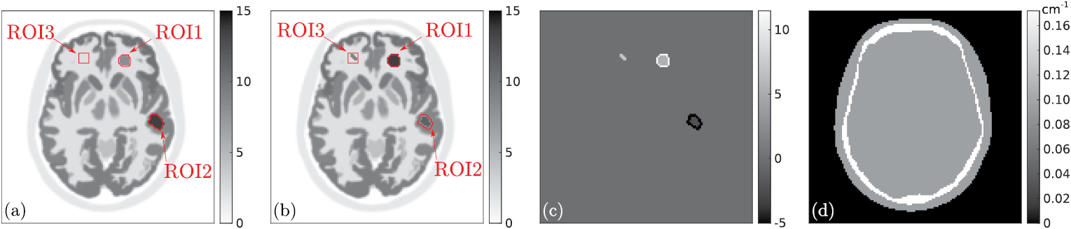
A realistic head phantom software (Rahmim et al 2008) was used to create discretised 2D activity and attenuation maps with a grid size of $128 \times 128$ pixels and an isotropic pixel size of side length 1.774 mm. By adding a number of hot spots to the initial activity map, the PET1 and PET2 ground truth images were defined (figures 1(a) and (b)). This resulted in three regions of change in activity distribution between the scans: a frontal-right region where an active tumour embedded in white matter increases in size and activity, a mid-right region where an active tumour embedded in grey matter decreases in size and activity, and a frontal-left region where a tumour appears. It should be noted that since the MAP-SLR methods do not distinguish the order of the two scans, PET1 and PET2 can be swapped without affecting the outcomes of the experiment.

Zoom In Zoom Out Reset image size

PET acquisition was simulated by forward projecting each of the ground truth images using the Radon transform. Attenuation factors, μ, for each scan were defined using the attenuation map shown in figure 1(d), with three pixel classes: air ($\mu={0}~{\rm cm^{-1}}$), water ($\mu={0.096}~{\rm cm^{-1}}$), and bone ($\mu={0.172}~{\rm cm^{-1}}$) (Burger et al 2002). Randoms were simulated as uniform sinograms and scattered events were modelled as smoothed copies of the forward projection of each image. The number of expected counts in each of the noise-free sinograms was ${{\sim}}$2.25 M, with $20\%$ from random and $20\%$ from scattered events.

3.1.2. Reconstructions and parameter selection.

Simulated noisy PET sinograms were reconstructed into images using the attenuation factors and randoms and scatters sinograms used in the simulations. All images were reconstructed into the same $128 \times 128$ grid as the ground truth images. For comparison purposes, the data were reconstructed using conventional ML-EM (Shepp and Vardi 1982) as well as the proposed MAP-SLR methods. In addition, double counts PET1 and PET2 datasets with an expected number of counts equal to ${{\sim}}$4.5 M were reconstructed with ML-EM to serve as a reference.

For the TV-MAP-SLR method, β values between $1 \times 10^{-4}$ and $1 \times 10^{-3}$ were used. For NC-MAP-SLR, β values between $5 \times 10^{-4}$ and $5 \times 10^{-3}$ were used, with σ values ranging from $0.5$ to $3.5$. All reconstructions were run up to 200 iterations.

3.1.3. Image evaluation.

For a set of images $\{\hat{\psi}_{jn}\}$ where $n = \{1, 2,...N\}$ Poisson noisy realisations of the simulated data, the reconstruction error relative to a ground truth image $\{\psi_j^{\rm GT}\}$ in a region $\Omega$ can be defined as a percentage root mean square error (%RMSE)

$$\begin{align} \displaystyle {\rm \%RMSE} = \frac{100\%}{N_\Omega} \sum_{j\in\Omega}{\frac{\sqrt{\frac{1}{N}\sum_{n=1}^{N}{\left(\hat{\psi}_{jn}-\psi_j^{{\rm GT}}\right)^2}}}{\psi_j^{{\rm GT}}}} \label{eq:rmse} \nonumber \end{align} \tag{ 8 }$$

where $N_\Omega$ is the number of voxels in $\Omega$. $N = 60$ noisy realisations of the data were used for reconstructions, and error levels were calculated across all non-zero pixels in the brain in the ground truth images (hereafter referred to as the whole-brain), as well as in regions of interest (ROIs) around each of the three regions of change. Specifically, these ROIs were: the front-right tumour (ROI1), the mid-right tumour (ROI2), and the front-left tumour (ROI3). These latter three regions are shown in figures 1(a) and (b) superimposed on the PET1 and PET2 ground truth images. Note that the same four analysis regions were used in both the PET1 and PET2 reconstructed images.

3.2. 3D tumour change experiment

The proposed MAP-SLR methods were then applied to real 3D data from a single FDG scan of a suspected frontal lobe epilepsy patient acquired on a Biograph mMR PET-MR scanner (Siemens Healthcare, Erlangen, Germany). The patient was injected with a total activity of 182.9 MBq and scanned for 30 min at 1.3 hr post-injection, resulting in a recorded total of ${{\sim}}$600 M prompt counts. Attenuation factors were estimated using an MR-based attenuation map generated from vendor-provided Dixon and ultra-short echo time sequences. Randoms and scatters were estimated with vendor-supplied tools using the delayed coincidence method and multi-slice 2D single scatter simulations respectively. Vendor-supplied normalisation files were also used in the reconstructions. Reconstructions and image analysis were carried out in MATLAB, with 3D mMR projections performed using in-house software (Belzunce et al 2015).

3.2.1. Dataset generation.

To create two pseudo-longitudinal datasets representing the PET1 and PET2 scanning sessions, the histogrammed patient data was split equally by randomly assigning each prompt count to one of two new datasets with equal probability. This resulted in two 3D Poisson distributed emission datasets whose sum was equal to the original data. Attenuation and normalisation factors for each of the split datasets were the same as for the original full-counts dataset. Randoms and scatters were defined to be $50\%$ of the original estimates.

Highly active tumours were then introduced to the same position in each dataset. For the PET1 dataset a spherical tumour with radius of 6.0 mm and additive intensity of $0.3$ was added (where the surrounding grey matter had intensities of approximately $0.25$). For the PET2 datasets, three tumour radii of 4.5 mm, 6.0 mm and 7.5 mm were defined, with additive intensities of $0.15$, $0.30$, or $0.45$. By using all combinations of intensity and size, nine PET2 tumours were simulated, allowing investigation of nine cases of longitudinal change.

3.2.2. Reconstructions.

The split datasets for each tumour change were reconstructed with both ML-EM and TV-MAP-SLR ($\beta=20$), with up to 100 iterations. In addition, reference images were obtained by adding tumours to the original dataset and reconstructing with 100 iterations of ML-EM (referred to as double counts ML-EM). All images were reconstructed into a $344 \times 344 \times 127$ grid with a voxel size of $2.08626 \times 2.08626 \times 2.03125$ ${\rm mm}^{3}$.

3.2.3. Image evaluation.

Images were analysed by measuring noise levels in two uniform regions of the reconstructed images. The first region was a 64 voxel region in the white matter and the second was a 32 voxel region within the highly active occipital grey matter. Noise in a given uniform region $\Omega$ for a given image $\boldsymbol{\psi}$ was quantified by using the coefficient of variation (CV) according to

$$\begin{align} \displaystyle {\rm CV}_\Omega\left(\boldsymbol{\psi}\right) = \frac{{\rm SD}_\Omega\left(\boldsymbol{\psi}\right)}{{\rm E}_\Omega\left(\boldsymbol{\psi}\right)} \label{eq:cv} \nonumber \end{align} \tag{ 9 }$$

where ${\rm SD}_\Omega\left(\boldsymbol{\psi}\right)$ is the sample standard deviation of voxel values of $\boldsymbol{\psi}$ in the region $\Omega$, and ${\rm E}_\Omega\left(\boldsymbol{\psi}\right)$ is the mean value in the same region.

In addition, the mean values in the tumour, white matter region, and grey matter region were recorded in PET1 and PET2 in order to observe the level of bias introduced by the TV-MAP-SLR method. Note that reconstructed image intensities using double counts ML-EM were halved prior to analysis to provide comparable regional means.

Ten realisations of the random splitting process were performed for each tumour change and the mean CV and mean values across realisations were used as final figures of merit.

3.3. 3D counts reduction experiment

The experiment described in section 3.2 was designed to explore the performance of the proposed TV-MAP-SLR reconstruction method for multiple tumour changes at a fixed level of counts (equal to ${{\sim}}$300 M per scan). In order to investigate the effect of the counts level on performance, a single case of tumour change from section 3.2 was selected and reconstructed with ML-EM and TV-MAP-SLR for various levels of counts per dataset. Specifically, the tumour change was a radius reduction from 6.0 mm to 4.5 mm, with an additive intensity reduction from $0.30$ to $0.15$ (as defined above). The original emission data was split into pairs of datasets by the same technique described above, with output datasets containing between $1\%$ and $50\%$ of the original ${{\sim}}$600 M counts each. The appropriately scaled tumours were then inserted into each of the datasets, resulting in a number of datasets nominally of the same object with varying counts levels.

Each of these pairs of datasets was reconstructed with 100 iterations of both ML-EM and TV-MAP-SLR with $\beta=20$. In order to analyse the PET1 and PET2 image quality across counts levels, the contrast to noise ratio (CNR) between the tumour and a background region in the adjacent grey matter was defined as:

$$\begin{align} \displaystyle {\rm CNR}\left(\boldsymbol{\psi}\right) = \frac{{\rm E}_{T}\left(\boldsymbol{\psi}\right)-{\rm E}_{B}\left(\boldsymbol{\psi}\right)}{{\rm SD}_{B}\left(\boldsymbol{\psi}\right)} \label{eq:cnr} \nonumber \end{align} \tag{ 10 }$$

where ${\rm E}_{T}\left(\boldsymbol{\psi}\right)$ denotes the mean tumour intensity within the mask used to define the tumour, and ${\rm E}_{B}\left(\boldsymbol{\psi}\right)$ and ${\rm SD}_{B}\left(\boldsymbol{\psi}\right)$ denote the mean and standard deviation in the background region respectively. A higher CNR is assumed to indicate a superior image quality since it indirectly measures the extent to which the tumour is visible against the surrounding tissue. Ten realisations of the data generation process were performed for each counts level and the average CNR across realisations calculated.

4.1. 2D simulation study

Figure 2 shows the PET1 and PET2 %RMSE values in the four analysis regions for ML-EM, double counts ML-EM, and TV-MAP-SLR with various values of β. Results are shown at iteration numbers corresponding to minimum whole-brain error and at 200 iterations. TV-MAP-SLR reduces whole-brain error relative to ML-EM both at minimum whole-brain error and at 200 iterations. As β increases, the error levels in the whole brain reduce, with the maximum β value of $1 \times 10^{-3}$ reducing minimum whole-brain %RMSE by an average of $11\%$ over both scans relative to ML-EM. At 200 iterations, the corresponding improvement is $22\%$.

Zoom In Zoom Out Reset image size

In the regions of change, the effect of the longitudinal TV regularisation is more varied. At the minimum whole-brain error iterations, %RMSE increases relative to ML-EM with increasing β in ROI1 (figure 2(a)) and ROI2 (figure 2(b)). In ROI3 (figure 2(c)), PET1 errors rise with increasing β whereas the PET2 error reduces. However, at 200 iterations the error in the tumour regions generally decreases with TV-MAP-SLR with increasing β, except for ROI1 in the PET2 reconstructions. In general, the increases in error levels in the regions of change are lower than the corresponding error reduction in the whole-brain error.

Figure 3 shows the error levels in the reconstructed images when using NC-MAP-SLR with σ values of $0.5$ and $3.5$. Similarly to the TV-MAP-SLR case, the whole-brain error decreases with increasing β for both σ values. When $\sigma=0.5$, similar trends to the TV-MAP-SLR case are observed, with %RMSE at minimum whole-brain error increasing with β in ROI2 (figure 3(b)) and in ROI3 in PET1 (figure 3(c)), and decreasing in the PET2 ROI3. In ROI1 however (figure 3(a)), the PET1 errors are reduced compared to the TV-MAP-SLR results in figure 2(a), both at minimum whole-brain error and at 200 iterations. Furthermore, although the general trends for the the NC-MAP-SLR method are similar to the TV-MAP-SLR results, the dependency on β is more non-linear. For β values beyond $2.5 \times 10^{-3}$, the behaviour changes, with errors at minimum whole-brain error changing more rapidly in ROI2 and ROI3. In fact, in ROI3 this change in behaviour causes the 200 iteration PET1 error to start to rise with β values greater than $3.5 \times 10^{-3}$. Overall, with β values up to $2.5 \times 10^{-3}$, the NC-MAP-SLR method with $\sigma=0.5$ performs similarly to TV-MAP-SLR, but with additional error reduction in ROI1.

Zoom In Zoom Out Reset image size

Increasing σ to $3.5$ degrades the performance of the NC-MAP-SLR method (figures 3(d)–(f)). The ROI1 error (figure 3(d)) increases with β in both PET1 and PET2 at minimum whole-brain error and at 200 iterations. In addition, the PET1 ROI2 error (figure 3(e)) at 200 iterations increases relative to ML-EM with any value of β, as well as errors at minimum whole-brain error rising faster with β than for $\sigma=0.5$. Furthermore, when $\sigma=3.5$ there is no region that experiences an error reduction relative to the $\sigma=0.5$ case.

Example reconstructed images after 200 iterations of each method are shown in figure 4 for ML-EM, double counts ML-EM, TV-MAP-SLR with $\beta= 6 \times 10^{-4}$, and NC-MAP-SLR with $\sigma=0.5$ and $\beta= 2.5 \times 10^{-3}$ and $4 \times 10^{-3}$. The selected regularisation parameters avoid excessive penalisation of the regions of change whilst demonstrating the benefits of the respective methods. For the NC-MAP-SLR method, the two β values were used to demonstrate the more complex relationship between error levels and β observed in figure 3. Figure 4 demonstrates that using the MAP-SLR methods improves the reconstructed images by reducing noise throughout the brain, approaching noise levels observed with double counts ML-EM. This is particularly clear in and around the striatum and is reflected in the difference images, where the amplitude of the background noise reduces when using the proposed MAP-SLR methods. Note that according to figures 2(a) and 3(a) the displayed NC-MAP-SLR reconstruction with $\beta= 2.5 \times 10^{-3}$ achieves on average slightly lower whole-brain error than the TV-MAP-SLR with $\beta= 6 \times 10^{-4}$ ($49.4$ and $50.7$ respectively) while also achieving lower error in ROI1 ($72.1$ and $73.5$ respectively). In addition, the corresponding NC-MAP-SLR difference image is sparser than the TV-MAP-SLR. Furthermore, increasing the β value to $4 \times 10^{-3}$ in the NC-MAP-SLR method produces an even sparser difference image; however the error levels in ROI3 at this penalty strength begin to rise again (figure 3(c)).

Zoom In Zoom Out Reset image size

4.2. 3D tumour change experiment

Figure 5 shows grey and white matter regional CVs and means for a range of iteration numbers for the 3D PET1 reconstructions using ML-EM, TV-MAP-SLR, and ML-EM with double counts. The mean values in these regions are improved by the longitudinal penalty, with TV-MAP-SLR producing regional means that agree with the double counts ML-EM reconstruction. In addition, using TV-MAP-SLR reduces the noise compared to standard ML-EM, with CV values almost identical to ML-EM with double counts at all iteration numbers.

Zoom In Zoom Out Reset image size

These improvements are evident in the reconstructed images (figure 6). Image-wide noise at 100 iterations of TV-MAP-SLR is visibly reduced when compared to 100 iterations of ML-EM with the same split data, to the point where the TV-MAP-SLR reconstructions are visually similar to the double counts ML-EM images. In addition to demonstrating reduced image noise, figure 6 shows that the visual appearance of the tumour is unaffected by the applied longitudinal regularisation. Inspection of the difference images confirms this observation, with the region of change remaining clearly visible.

Zoom In Zoom Out Reset image size

In terms of the quantification of the tumour, figure 7 shows the tumour means along with white matter CVs for all tumour changes for all methods at 100 iterations. For the case corresponding to figure 6, where the tumour reduces in radius to 4.5 mm and additive intensity to $+0.15$, a slight bias is introduced into the TV-MAP-SLR reconstructions so that the PET1 tumour mean is underestimated by 2.2% and the PET2 tumour mean is overestimated by 2.6% relative to the double counts ML-EM reconstructions.

Zoom In Zoom Out Reset image size

For the other tumours the regional means are either slightly biased towards the longitudinal average, or they agree with the double counts ML-EM value. The largest observed percentage bias relative to the double counts reconstruction was $-6\%$ for the PET1 tumour when the PET2 tumour was 7.5 mm in radius and $0.15$ in additive intensity, with all other bias magnitudes less than $5\%$.

4.3. 3D counts reduction experiment

Figure 8(a) shows the measured PET1 and PET2 tumour to background CNRs for count levels equal to $1\%$ of the original dataset up to $50\%$ (i.e. the case shown in figure 6) for ML-EM and TV-MAP-SLR. At all noise levels, and for both PET1 and PET2 reconstructions, TV-MAP-SLR was observed to produce a higher CNR than the corresponding ML-EM reconstructions. Visual inspection of reconstructed images at the $15\%$ counts level case (figure 8(b)) reflects these improvements, with the tumour more visible in the TV-MAP-SLR reconstructions due to a reduction of noise in both the adjacent background region and across the images in general.

Zoom In Zoom Out Reset image size

In this paper we have presented a new reconstruction paradigm for simultaneous reconstruction of longitudinal PET data. By penalising the differences between estimated images at each iteration we achieve the transfer of shared information. The proposed method was tested on a 2D simulation study which demonstrated that applying longitudinal regularisation improved the reconstructed images compared to ML-EM by reducing whole-brain error while maintaining or even reducing error levels in the regions of change. The decrease in whole-brain error is due to the noise reduction achieved by penalising longitudinal differences. By enforcing similarity between pixel values in PET1 and PET2, information from both datasets was used in each reconstruction, in effect increasing the number of counts available for each scan. Furthermore, by sharing this information using the selected prior functionals, the output difference images were sparser than those produced using traditional ML-EM reconstruction.

When using the TV-MAP-SLR method, the error levels in the two right tumours at minimum whole-brain error rose with increasing β, essentially creating a trade-off between error in the whole-brain and error in regions of change. This increased error in regions of change is because the TV prior penalises all differences equally, resulting in some degradation of the changes caused by tumour change. On the other hand, ROI3 in the PET2 reconstruction benefited from the TV regularisation due to improved reconstruction of the surrounding white matter. After 200 iterations of TV-MAP-SLR, error reduced in the mid-right tumour (ROI2) but increased in the front-right PET2 tumour (ROI1). This may be due to noise reduction occurring in the tumours as well as biases being introduced, so that in the mid-right tumour, where the magnitude of the ground truth change ($2.25$) is relatively low, the noise reduction is stronger than the bias, whereas for the front-right tumour where the corresponding change magnitude is $5.4$, the bias counteracts the noise reduction.

When using the NC-MAP-SLR method with $\sigma = 0.5$, whole-brain error again decreased due to a sharing of information between scans serving to increase the amount of data available for each image. However, in regions of change, the error levels at minimum whole-brain error were not as adversely affected as for TV-MAP-SLR, in particular in ROI1. The reason for this is the non-convexity of the prior that provides a derivative of zero at high changes. In terms of the iterative update in equations (6a) and (6b), this ensures that pixels with a large enough change revert to updates similar to ML-EM, and the cross-talk between scans in these regions is reduced.

However, as shown in figure 3, the NC-MAP-SLR method is sensitive to the values of β and σ; if β is too high, error levels can begin to rise more quickly with β (figures 3(b) and (c)), and with an excessive σ value the reconstruction penalises the differences we wish to maintain and the error levels also rise drastically (figures 3(d) and (e)). A good choice of σ is not necessarily obvious though, since it depends on the distribution of voxel changes due to noise and the magnitudes of the changes that are to be measured.

In addition, the non-convexity of the NC-MAP-SLR makes it a less robust option for reconstructing longitudinal datasets because the use of a non-convex prior can result in a number of local maxima in the objective function. The number and nature of these local maxima would depend on the sizes of σ and β, and it would be difficult to ensure that a global optimum were being approached for the reconstruction of any given dataset.

In the results for the 3D data experiment, using TV-MAP-SLR reduced image-wide noise to the same levels achieved when the number of counts was doubled and reconstructed with standard ML-EM. In general, for ML-EM reconstructions, noise reduces when the counts increase due to the signal-to-noise properties of Poisson distributions. The fact that TV-MAP-SLR reduced noise to the same level as doubling counts shows that the method is in effect sharing counts between datasets where the voxel-wise change is small enough.

In the tumour itself, the amount of bias introduced in the tumour varied depending on tumour size and intensity, with the largest observed bias of $-6\%$ in the case of increasing tumour size and decreasing tumour activity. In practice, the performance at a given tumour change is likely to depend on the strength of the regularisation, making future validation of these effects over a greater range of changes important.

As the number of counts per dataset reduced from $50\%$, TV-MAP-SLR continued to provide improved images, measured as an increase in tumour to background CNRs compared to ML-EM. There is the implicit assumption that the CNR accurately reflects the overall image quality, which may not be true when biases are present. For example, the results of the tumour change experiment (figure 7) show that longitudinal bias is possible when using the TV-MAP-SLR method. For the PET2 reconstructions, this bias is positive, with tumour means being increased relative to estimates from ML-EM. Using equation (10), it is clear that an increase in CNR can occur with either an increase in tumour mean or a decrease in background noise (given that the background mean is stable). Therefore, for PET2 reconstructions, the increased CNR could be due to a combination of both background noise reduction and the longitudinal bias in the tumour. However, the PET1 CNR values are also increased by using TV-MAP-SLR compared to ML-EM. In these images, tumour means should be biased negatively, lowering the CNR. The fact that the PET1 reconstructions exhibit higher CNR values even with the presence of this negative longitudinal bias suggests that the longitudinal biases are small relative to the noise reduction; and also confirms that the improvements in CNR seen for PET2 are primarily due to the noise reduction in the background as desired.

Overall, the experimental results of both the 2D simulated and 3D split real data studies show that there is generally a trade-off between reconstruction quantification performance in regions of change and regions that do not change when using the proposed MAP-SLR methods. The most suitable level of compromise will in practice be largely application-specific; metastasis localisation studies may be more tolerant to biases induced in lesions and benefit more from the increased CNR of the MAP-SLR methods, while studies where accurate quantification is of interest may benefit only a small amount (if at all) from coupling datasets in the reconstruction in the way described in this work. As such, it is clear that the proposed methods will require application-specific testing before being used in a clinical setting to ascertain (i) if there is a benefit to using MAP-SLR reconstruction methods in those contexts, and (ii) which level of regularistion is optimal. These considerations, while vital, are beyond the scope of this first exploratory study into longitudinal reconstruction methods.

From a technical point of view, the MAP-SLR methods presented in this work have some limitations that need to be addressed in future work. Firstly, MAP-SLR in its current form assumes that the majority of voxels are equal in intensity in both the PET1 and PET2 images. In practice, the injected dose in the PET2 acquisition is not necessarily equal to that of the PET1 acquisition. In this case, there would be a multiplicative factor for the intensities in one of the PET images that would provide the sparse difference image required. Future work will address this issue by including such a scale factor into the reconstruction, perhaps even simultaneously estimating the dose scaling factor during the reconstruction.

Another simplification used by the proof-of-concept experiments presented in this work is the assumed perfect alignment between the subject in the PET1 and PET2 datasets. This provides confidence that penalisation is applied to voxel differences that reflect only physiological change or change due to noise, and ignores the case where voxel values change due to a relative misalignment of anatomy. This limitation can be overcome by using anatomical information, such as MR images, to find the alignment operation and apply this in the reconstruction to obtain the correct differences. Alternatively, this misalignment could be estimated during the reconstruction (Jacobson and Fessler 2003, Blume et al 2010, Kalantari et al 2016).

Finally, the one-step-late nature of the proposed methods is not optimum because it is not guaranteed to converge to a maximum. For the TV-MAP-SLR method, defining an alternative, smooth prior that is TV-like at large changes and quadratic at small changes (such as the prior used by Wang and Qi (2015a)) would allow a more mathematically rigorous algorithm to be defined that is both guaranteed to converge to the MAP estimate and allows higher β values due to improved stability.

Nevertheless, the results presented in this work demonstrate that it is possible to improve reconstructed PET images by penalising differences longitudinally. For clinical studies where more than two scans are acquired, the MAP-SLR methods may be extended, potentially allowing even greater levels of noise reduction by sharing data from multiple PET datasets.

PET is frequently used to observe intra-subject longitudinal functional changes in a variety of contexts, including follow-up oncology scans to assess treatment efficacy. In this work, we propose a novel MAP PET reconstruction method to reconstruct longitudinal PET images simultaneously. The large degree of similarity between these datasets allows for information to be exchanged longitudinally in order to improve the reconstructed images by reducing noise. This was achieved by penalising differences between two longitudinal images during reconstruction in a one-step-late fashion, using both total-variation and non-convex difference penalties. The proposed methods, TV-MAP-SLR and NC-MAP-SLR, were demonstrated on 2D simulated datasets where lower whole-brain error levels were observed compared to ML-EM and error levels could be maintained in regions of change. In real 3D split datasets, with appropriate choices of hyper-parameters, the use of MAP-SLR reduced noise to effectively the level normally observed by using twice the number of counts while also maintaining regional means in a longitudinally variable inserted tumour.

Future work includes accounting for varying relative activity levels in the scans to be reconstructed, as well as spatial misalignment between the datasets. In practice, if adequately validated and tested, the proposed MAP-SLR reconstruction method may allow for reduced injected dose in routine clinical scanning protocols where multiple acquisitions over extended time-scales are required; or it may open up possibilities of scanning more vulnerable patient groups who are often excluded on the grounds of limiting radioactive dose.

This work was funded by the King's College London & Imperial College London EPSRC Centre for Doctoral Training in Medical Imaging (grant number EP/L015226/1) and supported by the EPSRC grant number EP/M020142/1. The authors would also like to thank Professor Alexander Hammers and Dr Colm McGinnity for providing the patient dataset. According to the EPSRC's policy framework on research data, figures and data supporting this study are openly available at https://doi.org/10.5281/zenodo.817457.