

Abstract
Direct imaging of the electrical activation of the heart is crucial to better understand and diagnose diseases linked to arrhythmias. This work presents an ultrafast acoustoelectric imaging (UAI) system for direct and non-invasive ultrafast mapping of propagating current densities using the acoustoelectric effect.
Acoustoelectric imaging is based on the acoustoelectric effect, the modulation of the medium's electrical impedance by a propagating ultrasonic wave. UAI triggers this effect with plane wave emissions to image current densities. An ultrasound research platform was fitted with electrodes connected to high common-mode rejection ratio amplifiers and sampled by up to 128 independent channels. The sequences developed allow for both real-time display of acoustoelectric maps and long ultrafast acquisition with fast off-line processing. The system was evaluated by injecting controlled currents into a saline pool via copper wire electrodes. Sensitivity to low current and low acoustic pressure were measured independently. Contrast and spatial resolution were measured for varying numbers of plane waves and compared to line per line acoustoelectric imaging with focused beams at equivalent peak pressure. Temporal resolution was assessed by measuring time-varying current densities associated with sinusoidal currents. Complex intensity distributions were also imaged in 3D.
Electrical current densities were detected for injected currents as low as 0.56 mA. UAI outperformed conventional focused acoustoelectric imaging in terms of contrast and spatial resolution when using 3 and 13 plane waves or more, respectively. Neighboring sinusoidal currents with opposed phases were accurately imaged and separated. Time-varying currents were mapped and their frequency accurately measured for imaging frame rates up to 500 Hz. Finally, a 3D image of a complex intensity distribution was obtained. The results demonstrated the high sensitivity of the UAI system proposed. The plane wave based approach provides a highly flexible trade-off between frame rate, resolution and contrast. In conclusion, the UAI system shows promise for non-invasive, direct and accurate real-time imaging of electrical activation in vivo.
Export citation and abstract BibTeX RIS
1. Introduction
Efficient pumping of blood is ensured in the heart by the synchronized contraction of the cells in response to electrical activation. Conduction disorders or arrhythmias correspond to a disruption in this activation sequence, which can have fatal consequences. One of the most prevalent forms of arrhythmias, atrial fibrillation, is associated with a 5-fold increase in risk of stroke (Fuster et al 2001). Other conduction disorders affecting the ventricles are associated with heart failure, which is the leading cause of hospitalization for patients above 65 years (Alla et al 2007). Non-invasive imaging of electrical activity remains challenging in patients. Electroencephalography (EEG) and electrocardiography (ECG) are used extensively in clinical practice to measure the electrical activity of the brain and the heart respectively. These techniques rely on highly sensitive surface electrodes to record voltage fluctuations resulting from neuronal ionic activation and cardiac cells depolarization respectively. However, both EEG and ECG are associated with limited spatial resolution.
Recent progress in ECG imaging using hundreds of electrodes have enabled imaging the electrical activation of the heart at an improved resolution, e.g., by localizing pacing sites to within 7 mm (Ramanathan et al 2004). However this technique is limited to the reconstruction of the electrical field on a surface. A technique allowing for the direct mapping and tracking of the electrical activation of tissues would be a key tool in improving our understanding of these complex diseases, performing better diagnoses, and contributing to the development of novel therapeutic approaches.
The acoustoelectric effect (Jossinet et al 1999, Lavandier et al 2000) is a phenomenon in which the propagation of an acoustic wave results in the localized modulation of the underlying medium's electric impedance. The local intersection of the acoustic wave with the current density can therefore be detected as an ultrasound-frequency variation of the voltage measured by a pair of remote electrodes. A few recent studies have demonstrated that this effect can be used to obtain images of the current density via methods such as Joule heat mapping (Yang et al 2012a, 2014) or directly (Olafsson et al 2008, Yang et al 2011, 2012b). In addition, studies have investigated the feasibility of leveraging the acoustoelectric effect for the imaging of biological tissues ex vivo (Olafsson et al 2007, Witte et al 2007) using standard ultrasound techniques involving focused acoustic waves which are associated with limited frame rates. Recent advances in ultrasound techniques (Tanter and Fink 2014) such as coherent plane wave imaging (Montaldo et al 2009), can be used to achieve frame rates up to 10 000 Hz without compromising the quality of ultrasonic images in terms of contrast, resolution and sensitivity. We have recently introduced ultrafast acoustoelectric imaging (UAI), which is also based on plane wave emissions (Provost et al 2014). Frame rates higher than 500 frames per second would be useful in tracking the propagation of the electrical activation in the heart, which typically occurs within 100 ms (Olafsson et al 2008, Provost et al 2011).
In this study, we have designed a UAI scanner, a fully-integrated compact system for high frame rate imaging of current densities using the acoustoelectric effect. A novel holographic image formation algorithm was used for the reconstruction of 2D images from a set of projections onto reference ultrasound plane waves, with a reconstruction speed allowing real-time display of images. The UAI scanner was characterized in terms of sensitivity, spatial resolution and contrast using a customized saline phantom. Finally, we showed the capability of our system to image time-varying electrical currents and complex current density distributions to demonstrate its potential for future in vivo applications.
2. Methods
2.1. Theory
2.1.1. The acoustoelectric effect.
The acoustoelectric effect, which was first reported by Fox et al (1946), results from the interaction between an acoustic wave propagating through a medium and a coinciding current density. Jossinet et al (1998) have further studied this effect and shown that the acoustic pressure change caused by the wave propagating locally modifies the medium's conductance following the equation below:

with  the conductance,
  the acoustic pressure variation and K an interaction constant (approximately 97 · 10−11 Pa−1 in saline (Jossinet et al 1998)).
According to Ohm's law, the voltage change V measured by a remote pair of electrodes can be written as the product of the medium resistivity ρ (inverse of the conductance) with the current density J integrated over the volume measured by the electrodes:

Following equation (1), the resistivity change from its initial value before perturbation by the ultrasound wave is:

Taking into account the contribution of the electrical current density and the electrodes field of view (FOV) into the expression of J, the voltage change V measured by a remote pair of electrodes can therefore be modeled by the following equation:

where  is the electrode field density and
  the current density. The first part of equation (2) corresponds to a low frequency term and can be filtered out in order to retain the high frequency and thus high resolution acoustoelectric signal (Olafsson et al 2008).
2.1.2. Acoustoelectric image formation using plane waves.
UAI is based, like ultrafast ultrasound imaging (UUI), on the use of ultrasound plane waves to form an image. Hence, each emission can be used to map the entire FOV, leading to frame rates that can be equal to the pulse repetition frequencies (PRFs), i.e. up to 10 000 Hz. Plane waves can also be emitted at different angles and resulting echoes are coherently compounded within the beamforming process to produce a high quality image of the object. UUI can produce images with resolution and contrast comparable to focused ultrasound for a limited number of angles, thus maintaining a high frame rate (Montaldo et al 2009).
Similarly, the concept of coherent compounding can be applied to UAI. Ignoring the elevational direction z in equation (2) above, the measured voltage difference due to the acoustic pressure variation can be written as follows:

with  , J the current density resulting from the convolution of the electrodes field and the current distribution, P0 the pressure amplitude and P the pressure field. Considering a plane wave emitted with an angle θ relative to the transducer array and the coordinates q and ct representing the wavefront, as pictured on figure 1(a), equation (3) can be rewritten as:

where RT [J] is the Radon Transform of J, c is the acoustic wave velocity, t is the time, and δ is the Dirac distribution.
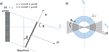
Figure 1. (a) Representation of the plane wave emitted with angle θ relative to the transducer array and relationship between coordinates, (b) k-space representation of the imaging limitations due to the finite emission bandwidth Δw and the limited angles that can be emitted.
Download figure:
Standard image High-resolution imageUltrasound arrays emit waves with a finite bandwidth, which leads to a convolution of the Radon Transform in equation (4) with a term W(ct) representing the emitted waveform:

Therefore, the Radon Transform is limited to regions of the k-space corresponding to the frequency bandwidth, as pictured in figure 1(b). This reduces the axial resolution of the system, which is linked to the ultrasound pulse length, as in focused ultrasound imaging.
In addition, the angular sensitivity of piezoelectric elements and the finite length of the transducer arrays limit the maximum angle at which plane waves can be emitted. This reduces the lateral resolution RL, which depends on the maximum angle θmax as follows:

where c is the speed of sound in the medium and fmax the transducer maximum frequency.
Finally, only a finite number of angles can be emitted in practice, which reduces again the sampling available for the RT as shown on figure 1(b). This affects the system's lateral FOV, defined here as the distance between grating lobes resulting from the pattern of interferences between the combined plane waves. The FOV is directly linked to the step between equally spaced angles  as follow:

As a consequence, although a larger maximum angle θmax ensures a better resolution (smaller RL), for a given PRF (i.e. number of angles), it also results in a smaller FOV.
2.2. The UAI system
2.2.1. Equipment.
The integrated UAI scanner is based on a 256-channel Vantage (Verasonics, Kirkland, USA) research platform fitted with a 128-element, 5 MHz linear array US probe (L7-4, ATL Ultrasound Inc., Bothell, USA) on one 128-element connector, and a break-out board allowing for the direct connection of individual channels on the second 128-element connector. The transducer was positioned with its pitch along the Y axis in order to direct the ultrasound pulse between the electrodes aligned along the Z axis, as depicted in figure 2. Channels 1–128 of the system were connected to the transducer and used for the emission of the acoustic wave. The 128 additional channels available via the break-out board were used in receive mode only to sample the UAI signal via measuring copper wire electrodes. The signal from the electrodes was high-pass filtered above 1 MHz and amplified using a high common-mode rejection ratio instrumentation amplifier and fed into the Vantage system via one selected channel of the break-out board with a gain of 1. Within the Vantage system, the signal underwent low-noise pre-amplification of 18 dB, controllable signal reduction at varying depth (set to 0 dB for all depths in the present configuration), and a subsequent amplification of 24 dB.

Figure 2. Experimental setup for phantom UAI measurements. Current was generated within a saline-filled pool via wire electrodes (red). Channels 1–128 of the Vantage system were used to emit plane waves. The UAI signal was measured by recording electrodes (black) placed on either side of the current electrodes, differentially amplified and sampled by the Vantage system via a single channel of the 128 channels break-out board. The right panel shows the alignment of the electrodes within the pool, perpendicular to the emission plane.
Download figure:
Standard image High-resolution image2.2.2. Holographic image formation.
The output of the integrated UAI scanner described above was used to form 2D images of the current density using a novel holographic image formation approach. This approach is analogous to optical holography in that it decodes the received signal by comparing it to a set of reference signals of known response by the system. It is based on the explicit construction of the direct problem matrix G, which links the object to image x and the demodulated complex measurement vector y as follows:

G is therefore a matrix with a number of columns equal to the number of pixels in the image x and a number of rows equal to the number of samples acquired. Since G approximately amounts to a bandlimited RT, as shown previously, the inverse problem is ill-posed and can be solved in a first approach using the pseudo-inverse formulation:

However, this consists in a deconvolution of the signal which is unstable, and may lead to added noise in the reconstructed image. G†G is a time-reversal operator and is thus close to identity if no ultrasonic absorption is considered during the building of G matrix (Tanter et al 2000). In more complex media where ultrasonic absorption occurs and results in degraded resolutions, the pseudo-inverse approach corrects for absorption effects through  inversion (Aubry et al 2001, Tanter et al 2001). Hence, the pseudo-inverse is similar to using a back-projection approach which amounts to projecting the time-reversed impulse response function such that

This formulation, however, does not take into account the individual pixels' energy. A more accurate approximation of the pseudo-inverse is the following:

In this case, the back-projection approach is normalized by the individual pixels' energy, without the need for deconvolution.
In the context of this work, the holographic image formation method was used for direct reconstruction of the 2D acoustoelectric image from a single acquisition channel only used in receive mode. Building G for a given emission waveform and imaged medium involves defining a set of basis vectors for the object space and determining the system response for each of these vectors. This was done using the Vantage system tool to simulate the emitted pressure waves and their value for each pixel. The simulation of one pixel allowed for the population of a single column of G. The integrated UAI scanner records the local voltage linked to the direct interaction of the acoustic wave and the current density, so only the transmitted waveform was of interest to construct G. The rows for each column (i.e. pixel) represent the transmission for each of the emitted plane waves along the whole FOV depth. As a consequence, the number of rows in G depended only on the number of plane waves emitted, and the imaging depth. The size of G in this work was therefore sufficiently small to allow for minimal computing time. Similar techniques have been used previously for sonar mapping (Tondin et al 2015), adaptive focusing in therapeutic ultrasound (Seip et al 1994) and image quality enhancement for medical ultrasound (Viola et al 2008), as well as for studies involving compress sensing, but to our knowledge, it is here applied to the reconstruction of UAI images for the first time.
2.3. Characterization of the setup
The UAI system was characterized in terms of sensitivity, resolution and contrast. Sensitivity was assessed by measuring the UAI signal in a configuration corresponding as much as possible to realistic physiological conditions. The signal was measured in a 6 × 3 × 3 cm3 3D-printed acrylonitrile butadiene styrene plastic pool filled with saline solution (0.9% NaCl). DC current was injected via a pair of tinned copper wire electrodes positioned within the solution using an arbitrary function generator (Tektronix AFG 3101, Tektronix Inc. Beaverton, USA) for amplitudes ranging from 2 to 20 V. A 100 Ω resistor was connected in series with one of the current injecting electrodes to measure current.
The peak negative and positive pressure of the plane wave imaging sequences were measured with an optical heterodyne interferometer, built and validated at our institution (Royer et al 1992), for an US probe voltage of 50 V which was the maximum used in this study. The peak pressure did not exceed 3 MPa, and was therefore lower than the limit of 4.7 MPa set by FDA requirements at 5 MHz (Harris and Philips 2008) for in vivo studies, corresponding to the derated value of 1.9 of the mechanical index (MI), with an MI value of 1.3. Conversely, the maximum recommended PRF corresponding to a spatial peak temporal average intensity (Ispta) of 720 mW cm−2 as recommended by the FDA in vivo was 19 000 Hz for an ultrasound probe voltage of 50 V. The values used in this study were therefore well within FDA recommendations to limit tissue damage, both in terms of MI and Ispta.
The ultrasound pulse was typically emitted at 3 MPa (MI = 1.3) with 128 elements corresponding to the L7-4 transducer. For sensitivity evaluation, the transducer peak pressure was varied between 3 MPa (MI = 1.3) and 0.3 MPa (MI = 0.13) for an injected current of 7 mA using three batteries connected to the electrodes. Series of 33 plane waves with angles varying between −8° and +8° were emitted at a frame rate of 200 Hz. Images were reconstructed using the holographic image formation technique described above.
Resolution and contrast were evaluated for a number of plane waves varying between 2 and 33. The value of  was set at 1° since it corresponded to the minimum value for which a 2 × 2 cm2 FOV does not include any grating lobes. The ultrasound pulses were emitted at a PRF of 4000 Hz, corresponding to frame rates between 200 and 2000 Hz. The optical heterodyne interferometer described previously was also used to determine the US probe voltage yielding equivalent pressure peak values to using focused ultrasound at an US probe voltage of 50 V. Spatial lateral resolution was defined as the width of the −10 dB peak of the UAI signal measured on a profile drawn in the x direction (see figure 4(c)). The current was produced by a pair of thin wire electrodes separated by 3 mm, and was considered equivalent to a point source in the plane of the US probe. Care was taken to ensure that the ultrasound wave was emitted within the gap between the electrodes. The contrast was quantified in terms of signal-to-noise ratio (SNR) defined as follows:

where  is the standard deviation (SD) of the background region, which was defined as a 15 × 15 pixel region neighbouring the UAI signal, and Imax is the maximum pixel intensity within the UAI signal. SNR values were measured on 100 single frames, and mean (SD) values are reported. Measurements were compared to the contrast and resolution obtained using focused waves for an F-number equal to 2.
2.4. UAI of time-varying currents
To demonstrate the capability of our integrated UAI scanner to map current densities in real time, an arbitrary function generator (Tektronix AFG 3101, Tektronix Inc. Beaverton, USA) was used to generate sinusoidal currents in the phantom. A 3 Hz, 2.8 mA peak-to-peak sinusoidal current was first injected through a single pair of electrodes in the saline pool. Next, a 10 Hz, 2.8 mA peak-to-peak current was injected via two electrode pairs separated in the saline pool by a 0.5 mm-thick sheet of insulating material. A phase difference of 180° was set between the currents applied to the two electrode pairs, named EP1 and EP2. UAI measurements were performed at 3 MPa (MI = 1.3) for a  of 1° over 2.5 s for 33 angles at 500 Hz. The variation of the signal's amplitude was expected to be visible in the UAI signal, as it is directly linked to the current density (see equation (2)).
2.5. UAI of a complex current density distribution
The UAI scanner was used to image a complex distribution of current density generated via 4 pairs of current-injecting copper wire electrodes positioned around the recording pair and connected to three 9 V batteries. The current density was imaged with 33 angles with a peak negative pressure of 3 MPa (MI = 1.3).
3. Results
3.1. Experimental setup
The experimental setup described above allowed consistent and reproducible measurements. Figure 3 illustrates the reconstruction process of 2D UAI data from 1D UAI signal received by the electrodes (top), corresponding to a single channel of the Vantage system. The corresponding 2D UAI image obtained, given at the bottom of figure 3, shows the UAI signal localized within the FOV of the system, corresponding to the imaged current density. The data on figure 3, measured for 7 mA injected into the saline pool, were obtained for a single frame. Reconstruction of UAI data was no longer than 4.6 s for 100 frames of a 128 × 192 pixels image built using 33 coherently-compounded plane waves, on an Intel 2.5 GHz dual core processor.

Figure 3. Illustration of the UAI reconstruction process for a single frame of a 33 plane waves acquisition of a current density corresponding to a 7 mA injected current. The different steps show the acquired data for each plane wave (zoomed in for a single plane wave in the black insert) and the reconstructed image obtained, displayed in dB.
Download figure:
Standard image High-resolution imageWhen evaluating the sensitivity of the system, a signal was measured for current intensity values recorded as low as 0.56 mA with a mean (SD) SNR of 6.0 (3.6) over 100 single frames. When varying the US probe voltage, signal was observed down to a value of 0.3 MPa (MI = 0.1) with a mean (SD) SNR of 5.2 (3.1) over 100 frames.
3.2. Characterisation of the setup
3.2.1. Resolution.
Figure 4(a) shows the resolution measurements of UAI data for 3, 5, 7, 9, 13, 15, 21 and 33 plane waves emitted at different angles, compared to the case of focused acoustoelectric imaging. The maximum steering angle was 16° for 33 plane waves. Examples of reconstructed images are given on figure 4(b) for 9 and 33 plane waves with no averaging. The resolution was measured as the width of the −10 dB peak, as illustrated for the case of 33 plane waves on figure 4(c). The resolution improved (i.e. the peak width decreased) with the number of plane waves, reaching equivalent values to the focused wave case for 13 plane waves. The resolution improved for higher numbers of angles to reach values of 2.1 mm for 33 plane waves, corresponding to less than a third of the value obtained for focused waves at an F-number of 2.
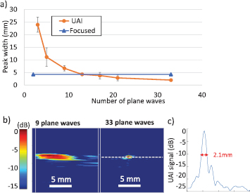
Figure 4. (a) Resolution measurements at different numbers of plane waves for UAI compared to the resolution for focused acoustoelectric imaging at equivalent peak pressure (the average over 100 frames is shown with error bars corresponding to the standard deviation), (b) reconstructed UAI data obtained for 9 and 33 plane waves (single frame), (c) profile corresponding to the white dashed line drawn on the 33 plane waves image, and measurement of the lateral −10 dB peak width indicated in red.
Download figure:
Standard image High-resolution image3.2.2. Contrast.
Figure 5(a) shows the SNR measured in the UAI images obtained previously for different numbers of plane waves. The SNR increased with the number of plane waves to reach a value 27 dB higher than for focused waves, for an F-number of 2. The SNR for UAI reached a similar value to the focused waves case when 3 plane waves were coherently compounded.
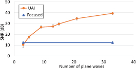
Figure 5. (a) Contrast measured on UAI data at 50 V for 27 V injected measured for varying numbers of angles, and comparison to the focused waves case at equivalent peak pressure. The average over 100 frames is shown with error bars corresponding to the standard deviation.
Download figure:
Standard image High-resolution imageBoth resolution and SNR were measured on 4 different datasets acquired with the same experimental setup and protocol, but with new tinned copper wire electrodes each time. Standard deviations (in percentage of the mean value) between the mean values obtained over 100 frames for each dataset ranged from 7% (mean 19 mm) to 26% (mean 2.4 mm) for resolution and from 3% (0.56) to 13% (24,7) for SNR.
3.3. UAI of time-varying currents
Figure 6(a) shows the reconstructed data obtained from imaging a 3 Hz sinusoidal current, in a single frame corresponding to a current peak. The variation of the UAI signal at the maximum intensity pixel is shown on figure 6(b) over 400 frames corresponding to 2 s. The UAI signal followed the sinusoidal form of the current with the same frequency.
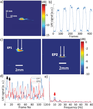
Figure 6. (a) Reconstructed UAI image from a 10 Vpp, 3 Hz sinusoidal current. (b) UAI signal measured at the maximum intensity pixel over time. (c) Reconstructed UAI data interpolated to a pixel size of λ/10 at electrode pairs EP1 and EP2 shifted by 180° in phase (white arrows indicate the position of the electrodes), (d) UAI signal measured at maximum intensity pixel for both electrode pairs (black arrows show frames corresponding to images on (c)) and (e) Fourier spectrum of the signal for EP1 and EP2. Red arrows indicate visible frequency peaks.
Download figure:
Standard image High-resolution imageFigure 6(c) shows reconstructed UAI data corresponding to the 10 Hz sinusoidal current injected via neighbouring electrode pairs EP1 and EP2 separated by a thin sheet of insulation. The images correspond to the frames indicated by the black arrows on figure 6(d), which shows the UAI signal measured at the maximum intensity pixel over time for EP1 and EP2. The 10 Hz sinusoidal waveform can be observed in the UAI signal, as well as the 180° phase shift between the electrode pairs. Figure 6(e) shows the Fourier spectrum of the signal obtained for EP1 and EP2. The peak at 10 Hz is visible and indicated by the red arrow.
3.4. UAI of a complex intensity distribution
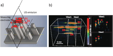
Figure 7 shows the complex intensity distribution imaged with the UAI scanner at 3 MPa (MI = 1.3) with 33 angles. The current between the top, middle and bottom pairs of electrodes is clearly visible on the image. The current distribution D3 (see figure 7) between the most distant electrodes is apparent with lower intensity on the UAI image. Electrodes pairs at the top and bottom (according to figure 7(a)) pairs are at the same distance from each other, which is reflected on the UAI image by a similar shape of the intensity distribution.
Figure 7. (a) Drawing of position in the electrode holder of the measuring pair (center) and the 4 current injecting pairs used to image a complex intensity distribution (b) 3D UAI image of the intensity distribution projected onto a black background. Two 2D cross-sectional views taken at locations indicated by the white dashed lines are shown on the right. The 4 current densities corresponding to the electrode pairs are indicated on panel (a) with red ellipses and annotated on both panels as D1–D4.
Download figure:
Standard image High-resolution image
4. Discussion
This work presents a fully integrated UAI scanner (see figure 2), characterised in terms of sensitivity and capacity of producing accurate 2D and time-varying images of current distributions. Although 2D acoustoelectric images have been produced in previous studies, the system described herein relies on a single ultrasound unit both for the emission of the acoustic wave and for the reception and processing of the UAI data. This has the advantage of simplifying the overall system, making it compact and easily portable. It also provides very high frame rates for the tracking of transient and fast events such as the electrical activation of the heart.
We have shown using the UAI scanner, that 2D-acoustoelectric images can be produced for low current (0.56 mA) with an SNR of 6.0 and higher. This value is close to physiologically relevant current densities (Henriquez et al 1988), and was obtained without any amplification beyond the one present in the Vantage system. The total amplification used in this study was 42 dB, which is lower than values reported in the literature (Witte et al 2007, Li et al 2012). In addition, contrast, resolution and real-time images shown in this paper were obtained for a single frame, without averaging.
An SNR of 5.2 obtained for low peak pressures shows the promise of such a UAI scanner for application to in vivo imaging without damaging tissues. All further acquisitions were performed at a maximum of 3 MPa pressure peak, which is 36% lower than the maximum set by the FDA to reach harmless MI and Ispta values (for the PRFs used) and minimize the impact on biological tissues. Indeed, the use of plane wave insonification of the FOV avoids high focused peak pressure. Therefore, UAI yielded up to 4 times higher contrast and divided the resolution 2 fold for equivalent peak pressure when compared against focused ultrasound, even when using a small number of emissions (see figures 4 and 5). Although these measurements showed variability across experimental datasets (see section 2.2.2), the variations did not affect the shape of the SNR and resolution curves. Such variations were due to the difference for each setup in the current injecting electrodes for which the exact length and geometry could not be fully reproduced. The small difference in the current densities generated is therefore possibly responsible for these fluctuations, rather than the UAI system itself.
An additional advantage of the UAI's sensitivity is the ability to produce time-varying images at a high frame rate (up to 500 Hz, data not shown). This is possible not only due to the high frame rate provided by the emission of plane waves, but also because of the high sensitivity of the system, which provides high SNR even for a single frame. Figure 6 shows the accuracy with which current density of sinusoidal signals can be measured together with their frequency. The only limit to the accurate frequency measurement of rapidly varying currents is linked to the ultrafast frame rate. Indeed, aliasing will occur if the frequency of the current to image is higher than half the imaging frame rate, following the Shannon–Nyquist theorem. This was observed in practice using our UAI scanner. The rapid reconstruction process (approximately 13 ms per frame for 9 plane waves) allows for real-time display of the 2D current density images obtained with UAI, which represents an important feature for clinical applications. Future work will focus on imaging alternating currents and incorporating phase information into the measured data.
Finally we have shown in figure 7 an example of a complex current distribution, produced by 4 pairs of electrodes positioned around the recording pair. The 3 groups of close electrode pairs were clearly visible on the image, with intensity levels that relate to the distance between electrodes (for D3) and the distance to the ultrasound probe (D4 compared to D1). For example pairs D1 and D4 had electrodes separated by 0.6 cm, leading to similarly wide intensity distributions in the image. Electrodes D3 were separated by 1.8 cm, leading to thinner intensity distribution. Variability in the image can also be accounted for by the use of a fixed elevation focus and by differences in the geometry, insonification angle, and positioning of the electrodes, which could not be fully controlled.
Controllable phantom distributions with known current density patterns were used throughout the study, since this work aimed at presenting and characterizing our UAI scanner. Work is ongoing to apply the scanner to in vivo imaging and investigate its potential for clinical applications.
Acknowledgments
This work was funded by ANR, Projet 14-OHRI-0012-01, and by LABEX WIFI (Laboratory of Excellence ANR-10-LABX-24) within the French program 'Investments for the Future' under reference ANR-10-IDEX-0001-02 PSL.