
Abstract
The aim of this study was to characterize the behaviour of superparamagnetic particles in magnetic drug targeting (MDT) schemes. A 3-dimensional mathematical model was developed, based on the analytical derivation of the trajectory of a magnetized particle suspended inside a fluid channel carrying laminar flow and in the vicinity of an external source of magnetic force. Semi-analytical expressions to quantify the proportion of captured particles, and their relative accumulation (concentration) as a function of distance along the wall of the channel were also derived. These were expressed in terms of a non-dimensional ratio of the relevant physical and physiological parameters corresponding to a given MDT protocol.
The ability of the analytical model to assess magnetic targeting schemes was tested against numerical simulations of particle trajectories. The semi-analytical expressions were found to provide good first-order approximations for the performance of MDT systems in which the magnetic force is relatively constant over a large spatial range.
The numerical model was then used to test the suitability of a range of different designs of permanent magnet assemblies for MDT. The results indicated that magnetic arrays that emit a strong magnetic force that varies rapidly over a confined spatial range are the most suitable for concentrating magnetic particles in a localized region. By comparison, commonly used magnet geometries such as button magnets and linear Halbach arrays result in distributions of accumulated particles that are less efficient for delivery.
The trajectories predicted by the numerical model were verified experimentally by acoustically focusing magnetic microbeads flowing in a glass capillary channel, and optically tracking their path past a high field gradient Halbach array.
Export citation and abstract BibTeX RIS

Original content from this work may be used under the terms of the Creative Commons Attribution 3.0 licence. Any further distribution of this work must maintain attribution to the author(s) and the title of the work, journal citation and DOI.
1. Introduction
Targeted delivery of therapeutic agents has, in recent years, been an active area of research, with magnetic drug targeting (MDT) being proposed as a particularly promising technique for localizing therapy efficiently. Magnetically-loaded drug carriers that can be non-invasively manipulated by an externally applied field are potentially useful for a range of therapeutic or diagnostic applications where an increased local concentration at a specific treatment site has an enhanced effect (Lübbe et al 1996, 1999, 2001, Alexiou et al 2000, Pankhurst et al 2003, Dobson 2006). There are, however, a number of challenges to overcome before the technique can be considered clinically viable (Grief and Richardson 2005, Laurent et al 2014, Schleich et al 2015, Shapiro et al 2015). In particular, while it is well recognized that the carrier formulation needs to be optimized for the application (Pankhurst et al 2009, Stride et al 2009, Mangual et al 2010, Pouponneau et al 2011), it is increasingly apparent that the external magnet needs to be designed to generate a sufficient magnetic force over the target range to remove a useful proportion of carrier particles from the hydrodynamic flow of the circulatory system (Driscoll et al 1984, Hayden and Häfeli 2006, Sarwar et al 2012, Owen et al 2014). Also, in order to optimize MDT as a minimally-invasive drug delivery strategy, external magnets should be designed to minimize off-target side effects, and maximize the efficiency of drug delivered to the target tissue.
For this reason, it is important to understand the performance of magnetic systems by considering the dynamics of superparamagnetic particles in flow as they experience the force applied by a spatially-varying magnetic field. Mathematical modelling of magnetic particles in transport has previously been used to study parameters related to the capture efficiency (Cregg et al 2008, Nandy et al 2008, Mangual et al 2010, Garraud et al 2016), particle trajectories (Gleich et al 2007, Owen et al 2015, Sharma et al 2015, Tehrani et al 2015, Garraud et al 2016, Zhou and Wang 2016), local concentration variations (Cao et al 2012, Cherry and Eaton 2014), extravasation (Nacev et al 2011a) and combinations of these (Bose and Banerjee 2015a), as a function of the magnetic properties of the particle formulation, external magnet design or factors related to the physiological flow. Understanding the dynamics of particle capture and accumulation in magnetic drug targeting applications can be particularly useful for informing the design and optimization of magnetic assemblies (Nacev et al 2011a, Shapiro et al 2014, 2015). However, magnet optimization is usually assessed in terms of the total magnetic force generated over a spatial range of interest (Alexiou et al 2006, Hayden and Häfeli 2006, Häfeli et al 2007, Takeda et al 2007, Sarwar et al 2012, Barnsley et al 2015, 2016), and simulation studies often do not consider whether this leads to optimal delivery to the target volume.
In this paper, we develop a mathematical model for assessing the performance of a given magnetic targeting scheme, in terms of the capture efficiency, accumulation (concentration) distribution of captured particles and trajectories of magnetic particles influenced by different sources of magnetic field, over a range of physiologically relevant flow rates. We consider first a simple spatial distribution for magnetic force and derive an analytical expression for the trajectory of a magnetized particle in a laminar flow in three dimensions. We then use this to derive a semi-analytical expression for the capture efficiency and accumulation distribution in terms of a non-dimensional ratio that encapsulates the relevant physical and physiological parameters for a given MDT scheme. Our aim is to provide a simple metric for gauging the potential effectiveness of a magnetic targeting scheme for a given target. We subsequently expand this model to numerically simulate particle trajectories in the presence of arbitrary magnetic arrangements and verify our predicted trajectories experimentally by acoustically focusing magnetic microbeads in a flow channel to a single trajectory, and observing how their paths deflect in the presence of a high-field gradient magnetic Halbach array. Finally, we examine simulated accumulation distributions to assess the relative performance of magnetic designs that have previously been considered for drug targeting applications (Hayden and Häfeli 2006, Häfeli et al 2007, McBain et al 2008, Barnsley et al 2016).
2. Methods
2.1. Mathematical formulation
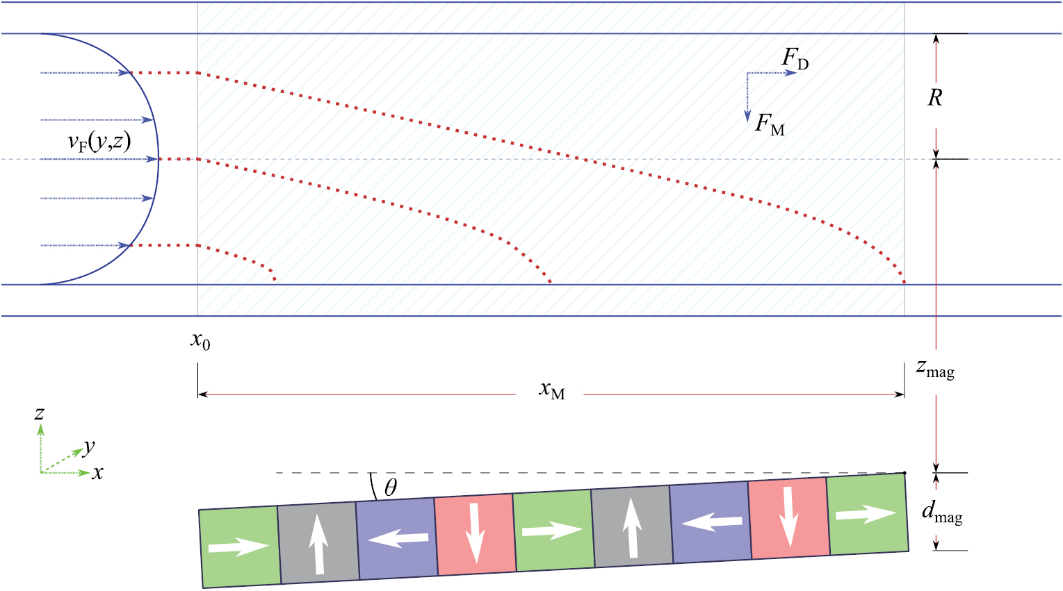
We consider a spherical, superparamagnetic particle suspended in a flowing liquid under the influence of an approximately constant magnetic force generated by a linear Halbach array (figure 1). The magnetic force along the channel is simplified to a step-function bounded by a range, xM from a starting position, x0 and acting in the -z-direction

Figure 1. The trajectories of particles within a flow channel of radius, R were calculated numerically. Flow was in the x-direction and the largest component of the magnetic field was parallel to the z-axis. The particles migrate under the influence of a drag force, a magnetic force, gravity and buoyancy. Unless otherwise stated, the magnetic field was simulated assuming a nine-element, linear Halbach array, set  from the centre of the flow channel. The shading highlights the spatial region bounded by
  in (1). The magnet was allowed to tilt around the trailing edge by θ, which is defined as the angle between the upper surface of the magnet and the bottom of the channel. Unless otherwise stated,
  and the magnet surface was parallel to the channel.
Download figure:
Standard image High-resolution imageIn a steady flow, the forces acting on the particle are given by

where  is the mass of the particle including the added mass,
  is the particle velocity and the four force terms on the right-hand side of the equation describe the magnetic force, gravity, buoyancy, and the fluid drag force respectively. We assume that
  and
and  is sufficiently small that the particle reaches terminal velocity extremely rapidly (so
  ). In a cylindrical channel carrying a laminar flow and positioned so that the central axis coincides with the x-axis, the flow velocity of the fluid is given by

where vA is the mean fluid flow velocity and R is the radius of the channel. Assuming a Newtonian fluid, the drag force on the spherical particle is given by Stoke's law:

where μ is the dynamic viscosity of the fluid, r is the particle radius. Combining (2) and (4) gives

The time-dependence of the position components,  and
and  is then determined by integrating the velocity components in (5) and setting a starting position vector described by
  , resulting in
We assume a no-slip condition so that the final resting position of the particle coincides with where the particle makes contact with the bottom surface of the wall (as the external force is directed towards −z), which occurs when  . Therefore, the final resting position is given by
which has one real solution for z0. The condition for which a particle can be considered to be magnetically retained is that the final resting position is within the bounds of the range of magnetic force, i.e.  .
.
We define the capture efficiency as the proportion of magnetized particles injected into the flow channel that are retained by the magnet. The capture efficiency was determined numerically by considering the final resting positions of an ensemble of particles initially distributed evenly about the cross section of the channel at the starting position, x0. This particular case is analogous to a 'capture cross-section' (Cregg et al 2008), i.e. the proportion of streamlines that terminate under the influence of the magnet. Other initial distributions are considered in appendix

where A = 0.601 and assuming that  does not exceed
  . (This expression has a similar form to one derived for a two-dimensional case by Nandy et al (2008), though their equation has an additional component which is sensitive to the spatial variations of the field source they considered). The accumulation distribution, which we define as the proportion of particles that accumulate in a range of positions between
  , is then

and has units m−1.
2.2. Numerical simulations
Typically, the magnetic force profile of a realistic magnetic system is not well described as a step-function. In order to predict the capture efficiency and accumulation distribution in MDT situations with a more physiologically relevant set of flow conditions and physically attainable magnetic forces, numerical simulations were performed to generate the trajectories of particles in a flow channel, under the influence of a position-dependent magnetic force. Simulations were performed using console applications written in the  programming language (Microsoft Corporation, Redmond, WA, USA). Numerical simulations can be performed in 3D with a much higher number of particles than comparable models solved using finite element methods (which can often be computationally prohibitive or highly mesh-sensitive and inaccurate when solving for fluid flow fields in 3D geometries (Nacev et al 2011a, Barnsley et al 2016)); typical simulations involving 2000 particle trajectories and 14000 unique time iterations completed in 2 h 40 min on a computer with an Intel(R) Core(TM) i7 processor and 8 GB RAM. The trajectories were determined at each time interval,
  by updating the position,
  , with
  calculated from an expression of a similar form to (5), but also taking into account gravity, buoyancy, and the spatial variation of
  :
:

The magnetic force from an arbitrary arrangement of magnetized elements was calculated using a model described and experimentally verified previously (Barnsley et al 2015), whereby the field,  was determined by breaking the magnet into a 3-dimensional lattice of evenly-distributed point moments, and summing the contributed dipole field at
  from each moment. In a curl-free magnetic field, the magnetic force on a particle with a magnetization,
  and volume, V is

The normalized magnetic force, used here for convenience because it has the same units as the field gradient (T m−1), is

where Ms is the saturation magnetization of the particle.
For simplicity,  and
and  were assumed to be parallel, and the particle was superparamagnetic so that the magnetization could be described using a Langevin function,
  ,
,

where  is the product of the Boltzmann constant and the temperature (Bean and Livingston 1959, Williams et al 1993, Majetich et al 1997).
For simulations using cylindrical channels,  was described analytically using (3). When a channel had a square cross-section, the flow profile was approximated by a
  expression, following the formulation of Lekner (2007) and setting the wall topology parameter
  ,
,
where w is the width of the channel and ϕ is the azimuthal angle. A 'sticky' condition was imposed for the wall, whereby particles that have made contact with the wall were assumed to be stable and no further updates were made to their position.
Numerical simulations were performed in which an ensemble of spherical particles modelling polystyrene microbeads loaded with a volumetric ratio (α) of superparamagnetic iron oxide clusters were evenly distributed at an injection point (Tehrani et al 2014, Bose and Banerjee 2015b, Lunnoo and Puangmali 2015) in a laminar flow contained within a straight channel aligned with the x-direction, and allowed to flow past a linear Halbach array consisting of nine rectangular, permanent magnet elements (figure 1). The magnet array was positioned a distance  away from the central axis of the channel and was designed so that, in the region of the channel above the magnet, the magnetic force was approximately, spatially uniform, provided the channel radius, R was sufficiently small. The main component of the magnetic force was aligned to the -z-direction, and gravity was directed perpendicular to both this direction and the direction of flow. A particle was considered captured if, when it came to rest at the channel wall, the magnitude of the magnetic force overwhelmed all others. The accumulation distribution was estimated as the relative proportion of particles lying within a range
  . This was done by taking the derivative, with respect to x, of a cumulative distribution function of the proportion of particles that were stable before reaching x (i.e.
  ). Inter-particle interactions were neglected.
Table 1 gives the default values for simulation parameters. The magnet array tilt angle, θ was defined as the angle made between the bottom of the channel and the upper surface of the magnet. Of the 18 parameters in table 1, 14 are used to calculate the final term in (10). In most cases, the default values of these parameters were chosen to be relevant to the experiments described in section 2.3. The effects of varying vA, FM (which depends on  ), R and θ on capture efficiency and accumulation are investigated in section 3.1, while section 3.3 explores the performance of different magnet array designs.
Table 1. Parameters used in numerical particle tracing simulations.
| Symbol | Description | Default value | Unit |
|---|---|---|---|
| μ | Fluid dynamic viscosity |  |
Pa.s |
| vA | Fluid mean flow velocity | 0.1 | m s−1 |
 |
Fluid density | 1000 | kg m−3 |
| R | Fluid channel radius |  |
m |
| V | Particle volume |  |
m3 |
| r | Particle radius |  |
m |
| ρ | Particle density |  |
kg m−3 |
 |
Fe3O4 density | 5240 | kg m−3 |
 |
Polystyrene density | 1050 | kg m−3 |
| α | Volumetric ratio of Fe3O4 | 0.1 | |
 |
Fe3O4 saturation magnetization |  |
A m−1 |
 |
NdFeB magnetization |  |
A m−1 |
 |
Magnet element dimensions |  |
mm3 |
 |
Distance to magnet | 3 | mm |
| xM | Magnet array length |  |
mm |
| θ | Magnet array tilt angle | 0 | ° |
 |
Gravity and buoyancy |  |
N |
| g | Gravity acceleration | 10 | m s−2 |
The ability of different magnet designs to target magnetic particles to a partially occluded vessel was also investigated by simulating trajectories within a symmetrically converging-diverging (or 'pinched') channel, shown in figure 2(b). The flow velocity inside a pinched channel was approximated following the derivation from Akbari et al (2010):

where R0 is the radius at the channel inlet and  is the radius at x. The channel has a constant slope on either side of the occlusion,
  .
.

Figure 2. Simulated channel geometries used to assess the ability of different magnet designs to deliver particles to a given position of interest (red circle). (a) The flow velocity in the straight channel with no occlusion and an inlet radius, R0 is described by (3). (b) A 'pinched' channel with a partial occlusion has a flow velocity given by (15). At the position of interest, the channel radius is set to half the inlet radius, while the total length of the occlusion is 4R0.
Download figure:
Standard image High-resolution image2.3. Magnetic trajectory experiments
Numerical predictions of trajectories were verified experimentally by flowing polystyrene magnetic microbead particles (2.0– m, Spherotech, Inc., Lake Forest, IL, USA) in a glass, square capillary channel primed with water (figure 3). Microbeads were diluted to a concentration of
  ml−1 and injected into a steady-flow field using a syringe pump. A dilute concentration was chosen to diminish the formation of agglomerated beads in flow (superparamagnetic beads are observed to interact weakly when separated beyond approximately six times their particle diameter (Oduwole et al 2016)). Acoustic focusing of the microbeads into a single trajectory was achieved by generating an ultrasonic standing wave (USW) field inside the fluid cavity of the channel using a lead zirconate titanate (PZT) piezoelectric transducer driven at
  MHz, using a linear frequency sweeping regime. Additional information about the design of the ultrasonic manipulation setup is reported in appendix

Figure 3. Microbeads were conveyed into a glass channel past a PZT transducer, which was actuated at approximately 2.6 MHz so as to generate an ultrasonic standing wave (USW) field within the fluid cavity. (a) In the absence of a USW, beads were unfocused and thus were located at different planes within the channel. (b) In the presence of the USW field, the beads are focused along a single trajectory by the action of acoustic radiation forces. (c) Schematic of the experimental set-up. A magnet positioned orthogonal to the viewing plane of the microscope deflects focused, magnetic beads towards the wall of the channel. (d) A purpose-built MATLAB image processing routine was implemented to determine the position of non-agglomerated microbeads recorded by the microscope.
Download figure:
Standard image High-resolution imageThe trajectory of the microbeads actuated by the Halbach array were extracted by a purpose-built MATLAB (The MathWorks Inc., Natick, MA, USA) image processing routine. Imaging scans along the channel length were analyzed frame by frame. Each frame was thresholded to separate magnetic particles from background. Objects greater than 250 pixels in area were discarded to exclude agglomerated magnetic beads and objects with less than 12 pixels were discarded as noise or refuse. Separate threshold levels were applied to isolate the top and bottom channel walls. Linear regression was used to extrapolate the top wall coordinates from the first 8 frames of the scan (before the Halbach array) since thresholding with magnetic particles accumulating at the wall of the channel was less reliable. The origin was taken as the midpoint between the top and bottom channel walls at the beginning of the first frame of the scan and particle centroid coordinates were recorded relative to this point. Non-magnetic particles that satisfied the size and thresholding criteria were rarely detected and manifest as outliers in the plots in figure 9.
Magnetic measurements were used to characterize the magnetic behaviour of the microbeads in suspension. Hysteresis loops of the microbeads were measured using a MPMS superconducting quantum interference device (SQUID) magnetometer (Quantum Design, Inc., San Diego, CA, USA) at a temperature of 270 K (in order to freeze the fluid) between ±1 T. The effective superparamagnetic particle size and volumetric loading of magnetite on microbeads were determined by fitting (13) to the hysteresis loop in figure A1, and these parameters were used to numerically predict the experimental trajectories reported in section 3.2.
3. Results
3.1. Simulation results
Numerical simulations were performed to ascertain the trajectories of magnetic microbeads in a steady, laminar flow, under the influence of the magnet array shown in figure 1, to investigate how the capture efficiency and accumulation distributions varied with the flow velocity, the magnetic force, the channel radius and the alignment of the magnet. The field and force profiles emitted by the Halbach array along the direction parallel with the upper surface, displayed in figure 4, show that, for a short range of z values, the 'step function' approximation used for the derivation in section 2.1 was reasonable. The results from the numerical simulations were compared with predictions using the expressions for trajectories, C.E. and accumulation distribution derived analytically.

Figure 4. Magnitude of the (a) field and (b) normalized force of the nine-element Halbach array shown in figure 1 as a function of x at different elevations, z from the upper surface of the array. The shaded range coincides with the region directly above the magnet array, and marks the space bounded by x0 and  for calculation of analytical trajectories.
Download figure:
Standard image High-resolution imageFigure 5 compares the analytically derived trajectories described by (6) and the simulated trajectories for average flow velocities of 10 and 20 mm s−1 and  set to 3 mm. The normalized magnetic force for the analytical trajectories was taken as the force directly above centre of the array at
  (
( T m−1). While the analytical expression made reasonable estimates of the final resting position of particles in flow, a few discrepancies are apparent, owing to the assumptions made in the derivation. The analytical trajectories generally underestimated xf on the near (negative) side of the magnet, and overestimated it on the positive side, which could be attributed to the variation of
  produced above the sides of the Halbach arrray. More importantly, the trajectory of the particle with the highest starting elevation shown in figure 5(a) (z0 = 2R/3) demonstrates how a particle could be both actuated and captured outside of the bounds of xM when a more physically realistic profile of
  was utilized. Once a particle was in a low flow regime, close to the channel wall, it slowed down significantly, and relatively little external force was required to pull it to the wall.

Figure 5. Predicted trajectories of particles in a cylindrical channel (R = 0.25 mm) initially set at various elevations, z0 along the z-axis, under the influence of the nine-element Halbach array and an average laminar flow velocity of (a) 10 mm s−1 and (b) 20 mm s−1. The symbols represent the trajectory given by the numerical simulation, while the line is described by (6). The shaded region is the same as figure 4, indicating where the 'step function' magnetic force (see (1)) operates.
Download figure:
Standard image High-resolution imageIn order to examine a wide range of possible trajectories, numerical simulations were run by initially distributing an ensemble of particles evenly around the cross-section of the flow channel upstream from the magnet, so that each particle had a unique starting  . Figure 6(a) shows how the travel distance of simulated particles (relative to the centre of the magnet, which defines x = 0) is related to their the initial position in the y-z plane at the injection point, with an average laminar flow velocity of 20 mm s−1. The colours indicate the final resting positions of the particles, xf, relative to the centre of the magnet. The particles that were initially furthest from the magnet (coloured white), and therefore had furthest to travel before being trapped at the channel wall, tended to pass over the magnet, reaching the outlet uncaptured. Alternatively, particles that had a very slow velocity near the bottom of the channel (coloured black) were removed from the flow by gravity before they reached the magnet. Analytical predictions for xf as a function of y and z0 using (7) for the same parameters are given in figure 6(b), and are qualitatively similar to the results of the numerical simulation. In both data sets, the proportion of particles trapped by the magnet in each 5 mm segment along the length of the channel (bounded by the counter lines) decreases with increasing x, indicating that more particles were trapped on the leading edge side (negative xf) of the magnet, and fewer made it to the trailing edge (positive xf).

Figure 6. (a) Colour-code to indicate the final resting positions (xf) of particles, overlayed onto a map of their starting positions in the y0-z0 plane cross-section of a cylindrical channel. The solid gray lines show contours of starting y0-z0 positions that have the same final position, xf. For this numerical simulation,  mm s−1 and
  mm. Gravity acted in the -y-direction, and the magnetic force vector pointed in the -z-direction. Black particles left the flow before reaching the magnet, while white particles passed over the magnet uncaptured, exiting the flow at the outlet. (b) The predictions of xf as a function of y and z0 given by the analytical expression in (7), with the same value of vA and FM set to 93.9 T m−1. Gravity was ignored in the analytical case.
Download figure:
Standard image High-resolution imageCapture efficiencies were determined for a set of numerical simulations following the method described in section 2.2 and were compared with the values predicted by (8). Figure 7 shows how the capture efficiency varied as one of the experimental parameters, vA, FM, R or θ was changed while the other parameters were fixed to their default values (table 1). The agreement attained between the simulation results and the analytical predictions indicates that the formulation derived in section 2.1 can provide a good first-order approximation for the capture efficiency in regions where the magnetic force is (relatively) spatially uniform.

Figure 7. The capture efficiency predicted by numerical simulations (symbols) and the semi-analytical expression of (8) (lines), displayed after varying (a) average flow velocity, (b) magnetic force, (c) channel radius and (d) alignment of the magnet. The fixed, default parameters are given in table 1.
Download figure:
Standard image High-resolution imageThe discrepancy in figure 7(a) at low flow velocities was due to the influence of gravity in the numerical simulations causing a relatively large proportion of particles to be removed from flow by gravity before reaching the magnet. At flow velocities less than 10 mm s−1, no particle made it to the outlet of the channel; particles were either forced out of flow by gravity before reaching the magnet, or captured by the magnet once they reached it. If simulations with these conditions did not include gravity, the capture efficiency would be 100%, as suggested by the analytical expression. Figure 7(c) shows that, as the channel size increased, so did the deviation between the two models. This was attributed to the fact that, as the channel size increased, the assumption of a spatially uniform magnetic force was no longer valid, and the magnetic force at the bottom of the channel, closer to the magnet, became significantly stronger than the force at the top of the channel. The effect of varying the magnet array tilt angle, θ is displayed in figure 7(d). For  , the capture efficiency didn't vary significantly, but the accumulation distribution (figure 8(d)) did.

Figure 8. A comparison of the accumulation distributions for a subset of the simulations described in figure 7. The symbols give the results of the numerical simulations, while the lines are described using (9). The shaded region is the same as that defined in figure 4.
Download figure:
Standard image High-resolution imageAccumulation distributions, calculated for a subset of numerical simulations using the method described in section 2.2, are shown in figure 8, and are compared with the profiles predicted by (9). For all tested parameter sets, (9) goes to infinity at the leading edge of the magnet, x0, highlighting a major discrepancy between the two models. Almost all distributions exhibited a peak in density in a region close to the leading edge of the magnet and, downstream from this point the agreement between the numerical simulations and the analytical derivation was reasonably good in most cases where the magnetic force was spatially uniform. Exceptions to this can be observed in figure 8(b), where the channel was far from the magnet, and the normalized force was small, and in figure 8(c) for large channel radii, where the forces at the top and bottom of the channel were significantly different. Notably, in many simulations, a significant proportion of particles were captured in a region prior to the bounds of the spatial extent of the magnet. Also of note, the peak in density usually occurred in a consistent position for almost all distributions ( mm) and, provided the simulations were performed in a space where the magnetic force could be approximated by (1), the shapes of the profiles overlapped very closely when normalized to the peak density. This suggests that, while the proportion of captured particles is sensitive to physiological flow conditions inside the body (encapsulated in the parameters vA and R), the relative spatial distribution of particles that are successfully captured is determined by the profile of the magnetic force (
 ). This means that particle distributions could be tuned and optimized for a given application by engineering the spatial profile of the magnetic force, so that the greatest density of captured particles would coincide with the desired region of interest. One attempt to do this is shown in figure 8(d), by varying θ. By tilting the magnet away from the channel, so that the force was localized in the region above the trailing edge of the magnet, the peak position of accumulation distribution was shifted closer to the position
  . However, fewer particles were captured overall.
3.2. Experimental results
The numerically predicted trajectories of particles under the influence of laminar flow and magnetic force were verified experimentally by flowing magnetic microbeads in a glass square capillary channel with an internal width of 0.3 mm and focusing them using acoustic radiation forces generated by a USW field, upstream from a linear Halbach array. The USW field was created by a PZT transducer coupled to the glass channel approximately 8 mm away from the Halbach array, to separate the regions of the channel exposed to acoustic and magnetic forces (appendix  varied between 2 and 15 mm s−1 (a range of flow velocities seen in intratumoral blood flow (Shimamoto et al 1987)). Starting positions used to calculate numerical trajectories were determined by averaging the elevation and distance to the wall of particles upstream from the influence of the magnet. The magnet position relative to the channel was measured from scanned images recorded using a fluorescent microscope, with the magnet-to-channel distance,
  set at 3.9 or 4.6 mm (corresponding to field gradients of 45 and 23 T m−1 above the centre of the array).
Figure 9 shows the measured trajectories compared with the numerical predictions, based on a microbead with the magnetic properties measured in appendix  ) before being actuated by the magnet, resulting in a 1.2 mm spread of positions for particles that were forced to the wall by the magnet. By comparison, a 15 mm s−1 average velocity resulted in a 0.056 mm wide trajectory, and a 8.1 mm spread of final particle positions for the same magnetic force (figure 9(d)). Variations in particle size and magnetic loading may have also contributed to distributions in particle positions about the predicted trajectory, as they would impact on both acoustic and magnetic forces.

Figure 9. Experimental positions of magnetic microbeads focused into a single trajectory by acoustic radiation forces and deflected by a linear Halbach array were imaged using microscopy (blue symbols) and compared with numerical predictions (red lines). The distance between the centre line of the glass capillary channel and the face of the magnet ( ) was set to (a)–(d) 3.9 mm and (e)–(h) 4.6 mm. The average velocity in the capillary,
  was varied between 2 and 15 mm s−1. The shaded area represents the part of the channel adjacent to the Halbach array. The position-axis gives the distance along the channel away from the trailing edge of the piezoelectric transducer.
Download figure:
Standard image High-resolution image3.3. Comparison of magnetic systems
Simulations were performed to investigate how accumulation distributions would differ with different permanent magnet designs, in order to determine which shapes and arrangements result in the greatest concentration of particles in a localized region of interest. Figure 10 shows the six magnet designs explored here. All designs were constrained to have the same magnet volume as the linear Halbach array and, in the case of the button and rod magnets, the same spatial extent along x. For the cone magnet, the diameter and height were set to be equal. The cube magnet (figure 10(d)) had a magnetization vector that pointed along a face diagonal, and was orientated on its edge so that  pointed along z. The arrays in figure 10(e) and (f) were designed using a force optimization routine for arbitrary shapes (Barnsley et al 2016) and a position of interest set
  mm away from the upper surface of the magnet. One design consisted of a single, uniform magnetization, while the other was a Halbach array assembled using six segments with different, orthogonally aligned, magnetization directions.

Figure 10. Designs of various permanent magnet shapes and arrays, with dimensions in mm. Commonly available uniformly magnetized shapes are shown in (a)–(c); (d) exhibits a permanent magnet cube which is diagonally magnetized along a face. (e) Uniform and (f) orthogonally magnetized arrays, optimized for magnetic force at a 3 mm range. All arrays have the same volume as the linear Halbach array above, and, where appropriate, the same spatial extent, xM. (a) Button magnet. (b) Cone magnet. (c) Rod magnet. (d) Diagonal cube magnet. (e) Optimized uniform magnet. (f) Optimized Halbach array.
Download figure:
Standard image High-resolution imageThe field and force profiles generated at a distance  mm from the upper surface of each magnet are displayed if figure 11, which shows that the uniform button and cone magnets are not well suited to apply a high field gradient in a localized region (the field and force from the button magnet are strongest at the edges). The two optimized magnets generate the strongest fields in the centre of the channel, particularly the Halbach array, which has a full width at half maximum (FWHM) in force of 8.54 mm.

Figure 11. (a) Field and (b) normalized force of the various arrays displayed in figure 10, along the x-axis at a distance  mm from the face. The shaded region gives the extent,
  mm, commensurate with that of the linear Halbach array in section 3.1.
Download figure:
Standard image High-resolution imageNumerical simulations were performed using the different magnet designs with the default values for vA,  , R and θ (table 1). The channel was positioned so that the maximum flow axis was
  mm from the upper face of the magnet array. Accumulation distributions in figure 12 indicate that the optimized arrays are better suited for localizing particles in greater density around the region directly above the centre of the magnet. Of the uniform magnets, the button magnet was notable because most accumulation took place above the edges of the cylinder, where the forces were strongest, and almost no particles were collected towards the middle. The rod behaved similarly to the step-force (linear Halbach array) above, capturing more particles at the leading edge of the magnet, but still capable of distributing particles in the region bound by xM, suggesting that these designs could be practical for applications in which particles need to be delivered to a large, diffuse area. These include diagnostic or biosensing applications involving a combination of active and magnetic targeting strategies for precisely locating and imaging tumours (Gunasekera et al 2009, Schleich et al 2014, Xu et al 2016). The cone and cube magnets were able to concentrate particles to a confined region close to their upper edges, but the peak linear density was not competitive with that of the two optimized arrays, owing to the fact that the generated force profiles persisted only over a very short-range compared with the optimized arrays (Barnsley et al 2015).

Figure 12. Accumulation distributions for simulations with the default simulation parameters for vA,  , R and θ, using the various magnets shown in figure 10. The shaded region highlights the default extent of xM, which is also the length of the button and rod magnets. (a) Profiles resulting from a channel with no occlusion; (b) profiles from a channel with a partially occluded geometry shown in figure 2(b). The dark gray line at x = 0 marks the position of interest at the centre of the occlusion.
Download figure:
Standard image High-resolution imageThe ability of each magnet design to deliver particles to a partial occlusion is assessed in figure 12(b). In all cases, the accumulation distribution at the site of the occlusion is less than the 'no occlusion' case in figure 12(a), as the flow velocity in the narrow region of the channel is significantly greater, and the distance from the bottom of the channel to the magnet has increased, reducing the peak magnetic force inside the channel. Table 2 details the capture efficiencies from the simulations shown in figure 12. While the optimized magnets are still the best of the tested designs at delivering particles to the position of interest, they are also the designs most relatively compromised by the presence of the occlusion.
Table 2. Capture efficiencies of different magnet designs in the absence and presence of a partial occlusion. Simulations were performed with the default values for vA,  , R and θ in table 1. The design of the linear Halbach array is shown in figure 1, while the designs of all other arrays are displayed in figure 10.
| Magnet design | No occlusion (%) | With occlusion (%) |
|---|---|---|
| Linear Halbach array | 29.27 | 24.20 |
| Button magnet | 11.54 | 9.86 |
| Cone magnet | 7.01 | 5.55 |
| Rod magnet | 18.61 | 15.10 |
| Diagonal cube magnet | 12.07 | 9.69 |
| Optimized uniform magnet | 16.61 | 13.44 |
| Optimized Halbach array | 22.60 | 17.93 |
Notably, even when the accumulation distribution was tightly localized, it was still skewed slightly towards the leading edge of the applied field/force. Figure 13 shows how the accumulation distribution varies as a function of two physiologically-relevant parameters, vA and R in a channel with no occlusion. Again, when vA was varied (and all magnet related parameters were fixed), the shape of the accumulation distribution changed only very slightly. The accumulation distributions displayed in figure 13(a) overlap almost entirely when normalized to the peak density, with the position of the peak shifting by just ∼1.4 mm over three orders of magnitude in vA (the mean FWHM of all distributions was  mm). The shape of the distribution did change with R, particularly at large values toward 2.5 mm (figure 13(b)), owing to the fact that the bottom of the channel was only 0.5 mm from the magnet, and the force profiles at the top and bottom of the channel were very different.

Figure 13. Accumulation distributions collected by the optimized Halbach array (figure 10(f)) varying (a) channel velocity and (b) channel radius.  was fixed to 3 mm. The insets show the capture efficiency as a function of the varied parameter.
Download figure:
Standard image High-resolution image4. Discussion
Magnetic targeting in a channel was considered mathematically using a numerical and semi-analytical model for the trajectories of an ensemble of superparamagnetic particles subject to a set of external forces inside a straight, cylindrical channel and a channel with a partial occlusion, both containing laminar flow. For the semi-analytical derivation, a constant magnetic force was considered to act over a fixed spatial range inside the channel, allowing for the derivation of expressions for capture efficiency and accumulation distribution of magnetic particles in the channel, assuming an evenly-distributed range of trajectories at the starting position. In this derivation, the capture efficiency is well described in terms of a non-dimensional parameter representing the ratio between factors that promote capture (magnetic force, FM and length of magnet, xM) and factors that mitigate capture (average flow velocity, vA, channel radius, R and viscosity μ). Nandy et al (2008) also derived the capture efficiency of magnetic particles in flow, finding that for this case the capture efficiency was also well described by a power-law for a non-dimensional ratio of a similar form to (8) (with slightly different coefficients). However, their derivation was for two spatial dimensions, with an infinite third dimension perpendicular to the direction of flow and magnetic force, which was generated by a spatially-varying line dipole. Given that all of the factors that comprise the non-dimensional ratio can be readily characterized for a given magnetic drug targeting set up, a simple calculation can provide a good first-order approximation for capture efficiency in regions where the magnetic force is relatively constant, which is useful for determining the total quantity of a drug that can be delivered. Alternatively, where the desired quantities are either well-characterized or constrained, knowing the required magnetic parameters to achieve an intended capture efficiency is useful for the design stage of both the external magnet and the magnetic carrier properties, particularly given that the applied magnetic force typically decays rapidly with distance from the magnet, and increases with the total magnet volume (Alexiou et al 2006, Hayden and Häfeli 2006, Häfeli et al 2007, Barnsley et al 2016). As an example, our previous design for a double layer Halbach array (Barnsley et al 2015) produced a field gradient of 85 T m−1 at a distance of 2 mm, and 12 T m−1 at 20 mm. Even at this range, this still provides a useful force (using (8) and for the default particle and channel parameters in table 1, a capture efficiency exceeding 10% would be expected for flow velocities up to 130 mm s−1), but beyond this, the rapid drop in force (and, therefore, capture efficiency) with tissue depth exhibited by most magnets highlights one of the main challenges with conventional magnet systems for MDT.
Particle sizes in the mesoscopic size range (nanometres to microns) are seen as advantageous due to a favourable ratio between magnetic and Stokes' drag force for improved magnetic targeting (Kozissnik and Dobson 2013) and also the ability to formulate composites to carry a combination of drugs or be compatible with multiple targeting strategies (Wadajkar et al 2012, Schleich et al 2014). However, smaller particles (e.g. free drug macromolecules and nanoparticles) are preferable for delivery, as they are better able to extravasate from the circulatory system, and accumulate in tumours (Matsumura and Maeda 1986, Maeda 2012). Modelling of nano-sized magnetic particles has previously been used to account for observations seen in clinical trials when the properties of the nanoparticles (i.e. size and magnetic moment) were well characterized (Nacev et al 2011a, 2011b).
For simplicity, the analytic formulation considered a Newtonian fluid in a straight channel, but blood is non-Newtonian, contains red blood cells and vessels are only approximately straight over short distances; these aspects are typically described using a blunted flow velocity profile (Nacev et al 2011a), added viscosity terms in large vessels (Zhang and Kuang 2000) and networked vessel geometries (Ritter et al 2004, Grief and Richardson 2005, Bose and Banerjee 2015a) respectively. While these features weren't considered in this study, they can be easily accounted for using the numerical model. The numerical model is particularly useful for understanding the relative spatial accumulation of particles along the length of the channel in the vicinity of a given magnetic field source. Simulations for a linear Halbach array (which produces an approximately constant magnetic force in a spatial region close to the face of the array) suggest that, when particles flow in one direction inside a straight channel past the array, most of the particles are captured towards the leading edge of the array. The relative profiles of the accumulation distributions described in section 3.1 are mostly determined by the spatial variation of the magnetic forces within the channel; where parameters that do not influence the magnetic force are varied (in particular, vA), the absolute peak value of the accumulation distribution changes, but the shapes of the distributions are mostly the same (overlapping when normalized to the same peak value). Therefore, understanding the spatial variation of the magnetic field and forces generated by a given magnetic field source is critically important for predicting the ultimate localization of magnetic carriers in the vessel network around the target.
The simulation results comparing external magnet designs suggest that for assemblies in which either the magnetic field or force is approximately constant over a large spatial range, captured particles are more likely to accumulate in the region of a vessel closer to the edge of the magnet, rather than towards the middle. Similar effects have been utilized in microfluidic devices with external magnets to manipulate particles by tuning field profiles (Gassner et al 2009, Cao et al 2013). For MDT, this can be a problem in a realistic vessel geometry around a target, which can often be tortuous and ramified, meaning that, if most particles are captured in regions corresponding to the edges of a magnet, efficient delivery to a single target site may not be possible, mitigating the primary advantage of using a magnetic system for drug delivery. Essentially, a magnetic system that is not well designed and/or carefully orientated would remove the greatest proportion of particles from flow before they even reach the target. This is particularly problematic with button magnets (one of the most commonly available magnet geometries); the strong edge effects and weak central force arguably make it the least appropriate magnet shape for MDT applications. Magnetic systems that are able to confine magnetic forces to a rapidly-varying peak-force region appear to perform better in localizing a high concentration of captured particles to a well-defined site. Of the tested magnetic arrangements, the shapes 'optimized' (Barnsley et al 2016) for magnetic force appear to perform the best for localized accumulation, although it should be noted that the peak accumulation distribution does not scale linearly with magnetic force. This would represent the most efficient accumulation profile for drug delivery to a solid, spatially-confined region of diseased tissue.
This highlights the importance of imaging to provide active feedback of the accumulation of captured particles, to ensure that the alignment of external forces results in good co-localization between drug carriers and the target region during therapy (Schleich et al 2015, Shapiro et al 2015). Carrier formulations utilizing iron oxide nanoparticles are seen as particularly favourable because iron oxide generates negative contrast in magnetic resonance imaging (MRI) (Pankhurst et al 2003, Das et al 2008), but many systems proposed for magnetic targeting (permanent magnet or electromagnet arrays) are fundamentally incompatible with MRI instruments due to safety reasons (Schenck 2000), and while magnetic delivery using MRI gradient coils is actively being researched (Mathieu et al 2006, Martel et al 2007, Mathieu and Martel 2009, Pouponneau et al 2011), conventional MRI gradient coils aren't designed to generate sufficient magnetic force to capture nanoscopic particles in particularly high flow regimes, meaning that MRI is often used as a diagnostic tool after therapy (Chertok et al 2008, Wadajkar et al 2012, Fan et al 2013). Imaging protocols that are based on magnetic particle imaging (MPI) (Gleich and Weizenecker 2005, Biederer et al 2009, Sattel et al 2009) or ultrasound imaging using carriers that are simultaneously responsive to acoustic and magnetic stimuli (Stride et al 2009, Liu et al 2011, Fan et al 2013, Crake et al 2015, Lee et al 2015), could be seen as means to monitor carrier concentration and localization during therapy that are compatible with the intense magnetic forces generated by magnetic drug targeting systems.
Particle trajectories for superparamagnetic beads within physiologically relevant flow regimes have been studied previously using numerical models (Gleich et al 2007, Nandy et al 2008, Sharma et al 2015, Zhou and Wang 2016). In order to experimentally verify the numerical predictions made using our model, we used acoustic focusing to study the motion of magnetic microbeads along a single trajectory in the vicinity of a linear Halbach array. Good agreement was found between the observed particle positions and numerical predictions on the length scales of our experiment, with no fitting parameters outside of the magnetic microbead properties which were measured by magnetometry (appendix
5. Conclusion
An analytical expression for the trajectory of a superparamagnetic particle under the influence of a magnetic force and laminar flow was derived in three dimensions, which was then used to derive semi-analytical expressions for the capture efficiency and accumulation distribution of particles in terms of a non-dimensional ratio of the most relevant physical and physiological parameters for a given magnetic targeting scheme. The results of numerical simulations of an ensemble of magnetic particles in flow, actuated by a linear Halbach array emitting an approximately constant magnetic force over a known spatial range were compared with the predictions from the analytically derived expressions. This demonstrated that the analytical treatise can provide good first-order assessments of the viability of MDT situations.
The numerical model was used to assess a range of different external magnet system designs and orientations to examine which configurations are most capable of capturing a large proportion of magnetic carriers under various flow conditions, and accumulating them in a confined, localized region. While the relative accumulation distributions in different flow velocities were found to depend primarily on the magnetic force profile, the relationship between the magnetic force profile and accumulation distribution was nontrivial. It was found that, of the tested magnetic systems, assemblies that provide a large peak magnetic force that rapidly varies over a confined region perform best at concentrating magnetic carriers to a target region. Experiments showed good agreement between the trajectories predicted by the numerical model and observed by acoustically focusing magnetic microbeads in a glass capillary channel, which were deflected towards a high field gradient Halbach array.
Acknowledgments
The authors would like to thank J Fisk and D Salisbury for their contribution to the design and construction of the Halbach array and holder. The authors would like to thank Dharmalingam Prabhakaran of the University of Oxford for helping with magnetometry measurements of magnetic microbeads. The authors are grateful to the Engineering and Physical Sciences Research Council for supporting the work through grant EP/I021795/1. All supporting data are available through the University of Oxford ORA data repository at https://doi.org/10.5287/bodleian:bx9jQBJdo
Appendix A: Magnetic measurements
Measurements of the magnetization curve of polystyrene magnetic microbead particles acquired using a SQUID magnetometer are shown in figure A1. The observed magnetic response was fitted using a Langevin function, as described by (13), assuming that the magnetic phase was magnetite ( kA m−1 (Margulies et al 1996)). An effective superparamagnetic cluster size of 8.6 nm and weight loading of 16.2% (volumetric ratio of 4.9%) were obtained, which were used in the numerical simulations of trajectories in section 3.2.

Figure A1. M-H curve for polystyerene magnetic microbead particles measured at 270 K between ±1 T at a concentration of  ml−1. The symbols represent the magnetic measurement and the red line represents a fit to the data using a Langevin function (see (13)).
Download figure:
Standard image High-resolution imageAppendix B: Acoustic manipulation of microparticles
In this section we describe the assembly, operation and characterisation of the acoustic manipulation device employed to focus magnetic microbeads into a single trajectory by means of acoustic radiation forces. The device comprised of a squared cross-section borosilicate glass channel (length: 100 mm, internal width: 300 μm, wall thickness: 150 μm; VitroCom, Ilkley, UK), which was acoustically coupled to a piezoelectric transducer ( mm3, PZ26, Meggit PLC, UK) using a thin layer of epoxy resin (RX771C/NC, Robnor Resins Ltd., UK) cured at
  C for 24 h. The transducer was positioned at a distance of 11.4 mm from the inlet of the channel, and was actuated by a radio frequency (RF) power amplifier (55 dB, Electronics & Innovation, Ltd., USA) driven by a sine-wave from a programmable signal generator (33220A, Agilent Technologies Inc., USA). An oscilloscope (HM2005, Hameg Instruments GmbH, Germany) was used to monitor the applied voltage and the operating frequency.
A one-dimensional (1D) impedance transfer model implemented in MATLAB was employed to identify the operating ultrasound frequency (Hill et al 2002), while numerical simulations were performed using COMSOL Multiphysics 5.2 (Acoustic-Piezoelectric Interaction module, COMSOL, Inc, Burlington, MA, USA) to determine the two-dimensional (2D) acoustic pressure field.
The 1D model treats the device as a planar resonator (i.e. with plane waves travelling in the thickness direction only) and provides a relatively accurate identification of the thickness resonance frequencies of a multi-layered structure (Hill et al 2002). The model predicted a half-wave resonant frequency at ∼2.64 MHz, with the pressure minimum (corresponding to the focusing position of the microparticles) located at 140 μm from the bottom surface of the fluid cavity (figure B1).

Figure B1. Normalized pressure distribution through the thickness of the device obtained from 1D impedance transfer model, at a resonant frequency of 2.639 MHz. Blue = transducer; red = bottom glass surface; green = fluid cavity; black = top glass surface.
Download figure:
Standard image High-resolution imageThe resonant frequency determined from 2D numerical simulations was equal to 2.67 MHZ, which was very close to the 1D prediction. Moreover, numerical simulations confirmed the presence of one pressure node, which was located at approximately the mid-plane of the fluid cavity (see figure B2). Notably, figure B2(b) shows that the acoustic pressure field was highly localised in a region of the fluid cavity above the transducer, suggesting that acoustic radiation forces acting on the microbeads could be considered negligible as soon as the beads exited the acoustically active area of the channel.

Figure B2. Contours of magnitude of acoustic pressure in the fluid cavity of the channel, normalised with respect to the maximum value. Values were determined numerically (using the Acoustic–Piezoelectric Interaction module in COMSOL Multiphysics). (a) and (b) correspond to a zoomed-out and zoomed-in view of the pressure field in the fluid cavity, respectively. The gray region represents the position of the transducer.
Download figure:
Standard image High-resolution imageIn order to achieve robust device operation across the range of flow rates investigated and minimise the risk of device going out-of-resonance, the transducer was actuated using a frequency sweeping regime ( MHz) at a sweep period of 50 ms. At this operating regime, microparticles experienced forces acting both horizontally and vertically towards the centreline of the channel, which originated from gradients in the potential and kinetic acoustic energy densities respectively, as reported previously in very similar resonant cavities (Mishra et al 2014).
Appendix C: Capture efficiency with different initial conditions
A semi-analytical expression for capture efficiency was derived by considering the proportion of final resting positions of an ensemble of particles, determined using (7), initially distributed evenly about the cross-section at the starting position. For all tested combinations of parameters with an even initial distribution, the capture efficiency was found to be well described by (8). Three other initial distributions were tested, described in this appendix.
The even, or uniform, distribution is shown in figure C1(a). The other distributions were determined using probability distribution functions (PDF),  where
where  is the initial radial distance from the central axis of the channel. The PDFs were:


Figure C1. Various, initial distributions of 2000 particles at the inlet of the channel. (a) Even, uniform distribution used for most simulations reported above. The probability that a given particle has an initial distance from the central axis,  in each distribution (b) radially uniform, (c) linearly decreasing and (d) Gaussian is given in (C.1a)–(C.1c) respectively.
Download figure:
Standard image High-resolution imageAll values of  are equally likely for the radially uniform distribution, while for the linearly decreasing distribution, the probability of a particle starting at the centre is greatest and at the wall is zero. The Gaussian distribution has a standard deviation of R/2 and the
  term accounts for the fact that the probability of a particle at the channel wall (
 ) is not zero. All PDFs total 1 when integrated from the centre of the channel to the wall. Probabilistic particle distributions plotted in figures C1(b)–(d) display 2000 particles, but 25 000 particle trajectories were calculated to determine the capture efficiencies exhibited in figure C2. Figure C2 shows how all tested distributions depend on the non-dimensional parameter,
  and the initial distribution. The uniform (black) curve was fitted to the power law in (8). As the accumulation distribution can be determined from the derivative of
  with respect to x, this would suggest that the accumulation distribution would also depend on the initial particle distribution.

Figure C2. Capture efficiencies determined using different combinations of the non-dimensional parameter  and the different initial distributions shown in figure 17.
Download figure:
Standard image High-resolution image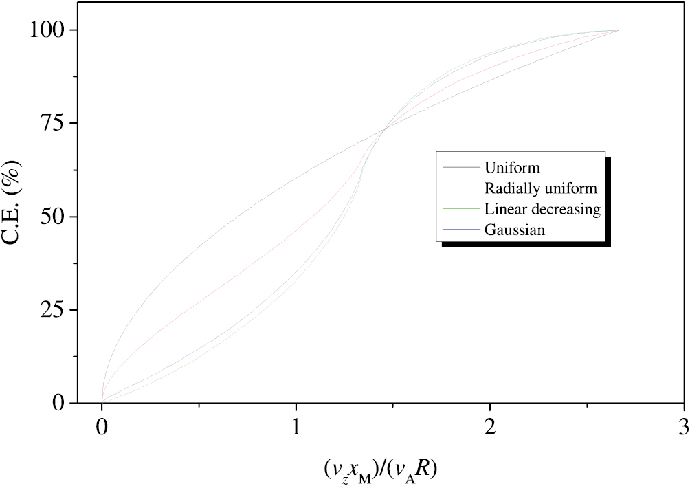