
Abstract
This study reports a novel method to measure and teach the specific heat by means of ordinary non-isolating containers and Arduino microprocessors. The measurements are managed by simply placing cold substances in hot water and by monitoring the instant temperature variation via the Arduino UNO microprocessor. This method is original in the sense that it employs ordinary non-isolating containers and obvious heat loss from the container is determined by mathematically modelling the temperature decrease as a function of time. The specific heat measurements are managed based on the heat energy exchange between the hot water and the cold substance by extracting the heat loss to the environment. Proposed method is specifically employed for the substances of aluminium and copper and the measurements revealed that the relative errors of the measurements are 6.50% for copper and 1.38% for aluminium. This novel approach is very easy to implement, inexpensive and can effectively be employed on teaching physics, science and engineering. The novel method can also be employed on basic research activities and industrial applications.
Export citation and abstract BibTeX RIS

Original content from this work may be used under the terms of the Creative Commons Attribution 4.0 license. Any further distribution of this work must maintain attribution to the author(s) and the title of the work, journal citation and DOI.
1. Introduction
Physics deals with all sorts of phenomena encompassing energy or matter and resolves relating concepts and natural laws, develops theories that can predict the results of experiments (Sears et al 1974, Serway and Jewett 2018). Physics is naturally and generally considered to be problematic due to involvement of complicated concepts and lack of adequate uncomplicated experiments in teaching processes (Fishbane et al 2003, Prensky 2005, Veloo et al 2015, Vilia and Candeias 2020). Therefore, physics education research aims to identify the topics that students experience difficulties in learning and tries to reduce complications and also aims to educate students with competencies required by the society. It is hence important to address difficult-to-understand subjects in physics education with novel and simple methods and approaches (Marioni 1989, Lewis and Linn 1994, Wieman and Perkins 2005).
One of the most problematic sub-sections of physics is thermodynamics. Thermodynamics, deals with macroscopic properties of matter namely temperature, heat, internal energy, thermodynamic work, pressure and volume etc. based on microscopic structure of matter. Therefore, it is considered one of the most challenging subjects that students experience great difficulties in learning and internalizing. (Barrow 1988, Lewis and Linn 1994, Viennot 1998, Alwan 2011). Specific heat and heat capacity are fundamental and very important concepts of thermodynamics, connecting heat and temperature and therefore ought to be internalized by means of adequate experimental measurements. Specific heat basically represents the amount of thermal energy per unit temperature and per unit mass ought to be exchanged by the substance. Therefore, the greater the specific heat of the substance, the more heat energy is needed to increase the temperature by 1 Kelvin. Thermal energy or the heat energy is, on the other hand, can alternatively be assumed as the overall micro mechanical energy of the particles of the substance, hence it has primary importance both scientifically and technologically. On the other hand, in order to improve students' experimentation skills in laboratory applications, it is surely important to provide teaching atmospheres full of collaborative learning and discussion (Deslauriers et al 2011).
It is standard approach of thermodynamics experimentation that the specific heat of a substance is measured by using an isolating container. However, isolating containers can always leak some amount of heat that violates the perfect isolation rule and causes great difficulties and measurement errors. Consequently, alternative methods that can eliminate the need of isolating container and the heat leakage are tremendous desire of the community of educators, researchers and also industrializers. Numerous studies have reported various alternative methods and approaches to measure and teach the specific heat and some of them are summarised as follows. Recently, the measurement of specific heat by means of Rüchardt's experiment has been reported (De Lange and Pierrus 2000, Severn and Steffensen 2001). Similarly, the measurement of specific heat through cooling curves has also been studied (Mattos and Gaspar 2002). More recently, a temperature relaxation method for the measurement of the specific heat of solids at room temperature in student laboratories has been developed and reported (Marıén et al 2003). Bisquert has developed and reported a master equation approach to the non-equilibrium negative specific heat at the glass transition (Bisquert 2005). Lately, a study is reported on measuring the specific heat of metals by cooling the substance (Dittrich et al 2010). Koser has studied and reported a laboratory activity based on specific heat by change in internal energy of silly putty (Koser 2011). Another recent study has reported high precision measurement of specific heat using dual heating and cooling (Shengjie et al 2017). Finally, an alternative approach on teaching specific heat using learning by laboratory activity is reported (Lohajinda et al 2019).
Arduino microprocessors, on the other hand, are devices that include digital and analog sensors, LEDs, motors and heating elements, where sensors and transducers are widely available. Arduino microprocessors are nowadays used at almost every level of education, technology and engineering. Arduino microcontrollers are electronic devices that can be programmed with C language and collect data from various sensors with the help of these electronic devices where very good work can be done with the introduction of robotic coding (Petry et al 2016). The importance of Arduino use in physics education rapidly increases due to being inexpensive, easy to apply and being coded by easy C language and the codes are globally available by open sources. For this reason, measurement tools and experimental setups can be designed with the Arduino microcontrollers and it can easily be employed in physics experiments. There are numerous recent studies reporting the use of Arduino in measuring and teaching various sub fields of physics education, namely mechanics (Çoban and Erol 2022, Erol and Oğur 2023), electricity (Zachariadou et al 2012), magnetism (Atkin 2016), optics (Gopalakrishnan and Gühr 2015), thermodynamics (Prasitpong et al 2022).
Consequently, the aim of this study is to introduce a novel method of measuring and teaching the concept of specific heat by means an ordinary container with no isolation and an Arduino microprocessor. This approach is a novel route to experimentally determine the specific heat by mathematically modelling the heat loss of the container to the environment and eliminating the loss to estimate the actual specific heat. This approach is believed to have substantial potentials for educational, scientific and technological applications.
2. Quantum theory of specific heat
Heat capacity, a fundamental thermal property of matter, is defined as the amount of heat energy given to or obtained from the substance in order to change the temperature of the material by 1 degrees Kelvin. The heat capacity of a substance, denoted by C, is defined by,
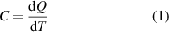
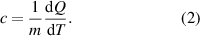
where dQ is the infinitesimal amount of heat exchanged by the substance to vary the temperature by dT. The amount of heat given to the system is obviously accommodated within the substance and maintained as the micro mechanical energy of the constituent particles and chemical bond energies of the particles. Therefore, the measurement of heat capacity is important to specify numerous physical and chemical properties of the substance. Accordingly, the specific heat of a substance is defined as the heat capacity per unit mass of the substance. The specific heat of a substance, usually denoted by c, is defined as the heat capacity of a substance divided by the mass of the substance,
Heat capacity and likewise the specific heat of a substance is due to the motion of the constituent particles which are, regarding the solid substances, bound with each other by chemical bonds and relentlessly vibrate around an equilibrium position. Theoretical resolution of the heat capacity was a bit of problem of classical physics however tackled and resolved by Einstein who treated the particles of the solid as non-interacting quantum harmonic oscillators vibrating with fixed frequencies. Einstein model of heat capacity resolved the main problem, which was the decrease of the heat capacity as the temperature decreases, nevertheless was unable to explain the whole temperature range from absolute zero to the room temperatures. The problem was later tackled by Debye, assuming the particles vibrating with different frequencies ranging from 0 to a maximum frequency of  . Accordingly, the mean internal energy which is equal to the heat energy of a single vibrating oscillator/particle can be calculated from,
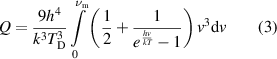
where  denotes the Debye temperature of the solid, h is the Planck's' constant, k denotes the Boltzmann's' constant,
  denotes the frequency and T denotes the absolute temperature of the substance (Kittel 2005). Accordingly, the heat capacity of the substance, which accommodates overall N particles, can be calculated by using the definition of (1) and by taking the first derivative of the internal energy/heat energy with respect to temperature, which yields,
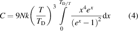
where  denotes the energy quanta divided by the thermal energy of the particle. This final expression can be approximated for high and low temperatures with respect to Debye temperature of the solid. At high temperatures, if the condition of
  holds then it means
  which leads to the simple result of,

which is known as Dulong-Petit law. The Dulong-Petit law expresses that at room temperatures and above the specific heat of solid substances is approximately equal to,
which is obviously constant. The specific heat at room temperature accordingly depends on the number of oscillators or vibrating particles, N, within the solid substance. The quantum mechanical calculation outlined above can be specified for any substance by taking into account of certain substance parameters such as the mass of the particles,  , and the energy of the chemical bond. Therefore, it is legitimate to express the mass of the substance, m, in terms of the mass of the oscillating atoms or molecules,

where  denotes the mass of the oscillating particle and N denotes the total number of particles within the substance. In this case, the specific heat of any solid substance can be given by,
This expression defines the specific heat of any solid state substance in terms of the mass of a single oscillating particle,  , articulating that the specific heat is inversely proportional to the mass of the oscillating particles.
3. Method
3.1. Experimental setup
The experimental setup is comprised of an ordinary computer with appropriate code loaded, an ordinary kettle, a precision scale with a sensitivity of 0.1 g, two thermometers, 2 beakers, Arduino Uno microprocessor, a DS18B20 waterproof temperature sensor, a breadboard, an Arduino Uno-computer communication cable, connecting cables, copper and aluminium substances and crucially an ordinary non-isolating container. The experimental setup including all the equipment is shown in figure 1.
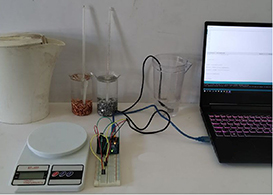
Figure 1. The photography of the experimental setup showing all parts used to carry out the measurements.
Download figure:
Standard image High-resolution imageThe actual substances of aluminium and copper are made up of small pieces, as shown in the figure 1, in order to easily let the heat energy transfer from the water molecules to the atoms of the substances. The non-isolating container is an ordinary one made up of plastic derivatives however can be made up of anything namely glass, ceramic, metal, plastic, or wood etc.
3.2. The Arduino and temperature sensor
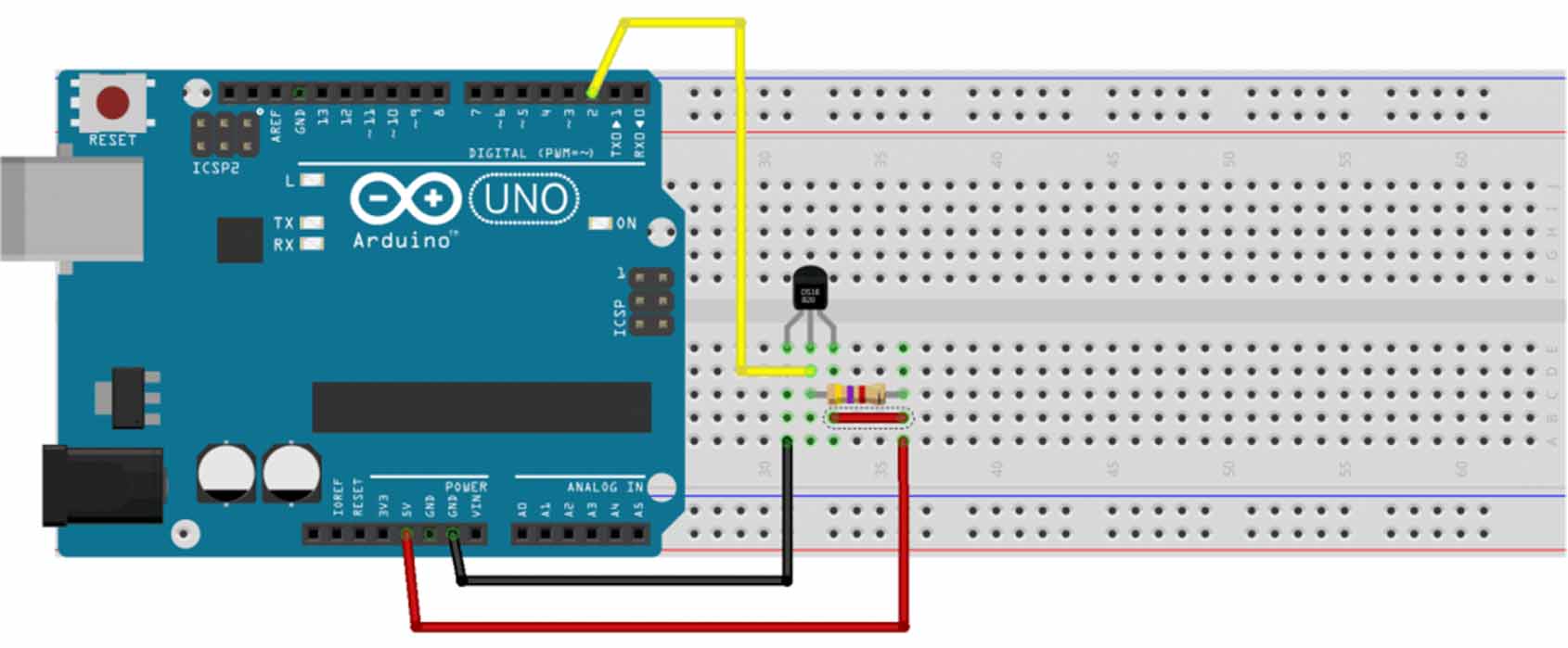
The Arduino microprocessor can obviously be used for many applications by appropriate codes and relevant sensors. In this case, Arduino Uno microprocessor is employed and the code specifically prepared for the DS18B20 temperature sensor is freely obtained from the Arduino Library. The photography of the actual wiring between the DS18B20 temperature sensor, the computer and the Arduino is shown in figure 2.
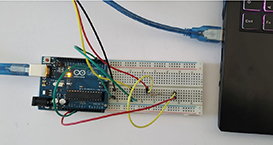
Figure 2. The connections and wiring of the temperature sensor, the computer and the Arduino Uno.
Download figure:
Standard image High-resolution imageThe illustration showing the details of the connections between the DS18B20 temperature sensor and the Arduino Uno is additionally shown in figure 3. The DS18B20 temperature sensor is a waterproof device and it sends 9 or 12-bit digit output via one-wire protocol. The DS18B20 temperature sensor measures temperatures from −55 °C up to +125 °C and converts 12-bit temperature to digital word in 750 ms. The resistor shown in the figure 3 used for the communication between the Arduino and the temperature sensor has a size of 4.7 kΩ.

Figure 3. The illustration showing the details of the connections between the DS18B20 temperature sensor and the Arduino Uno.
Download figure:
Standard image High-resolution image3.3. The code
The specific code for the DS18B20 waterproof temperature sensor is obtained from the Arduino library (www.arduino.cc/en/software) freely available for any researcher. However, the code is just revised due to the needed time scale to collect the appropriate data which is in this case 5 s. The actual code is presented below.
#include <OneWire.h>
#include <DallasTemperature.h>
OneWire oneWire(2);
DallasTemperature DS18B20(&oneWire);
DeviceAddress DS18B20adres; float santigrat, fahrenheit; void setup(void)
{
Serial.begin(9600);
DS18B20.begin();
DS18B20.getAddress(DS18B20adres, 0);
DS18B20.setResolution(DS18B20adres, 12);
} void loop(void)
{
DS18B20.requestTemperatures(); santigrat = DS18B20.getTempC(DS18B20adres); fahrenheit = DS18B20.toFahrenheit(santigrat);
Serial.println(santigrat); delay(5000);
}
3.4. Novel method for the specific heat measurement
The method employed in this work is an original and very low-cost one based on eliminating the heat transfer to the environment from the ordinary non-isolating container. The method is especially significant in the sense that firstly it needs no isolating container and any ordinary container can be employed for the measurements and secondly it employs Arduino microprocessors with appropriate temperature sensors which are efficiently inexpensive.
The measurement procedure is mainly based on mathematically modelling of the heat energy transfer from the non-isolating container to the environment and eliminating that heat energy loss. In order to mathematically model the heat loss of the non-isolating container, the container is filled with appropriate amount of hot water and system started to collect the temperature-time data. The gradual decrease of the temperature of the water is monitored by the Arduino as a function of time and specifically the temperature is measured every 5 s. The schematic representation of a typical graph for the time dependence of the temperature is shown in the figure 4.
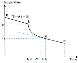
Figure 4. Schematic representation of a typical temperature versus time plot for a non-isolating container used to mathematically model the heat loss and to measure the specific heat of the substance.
Download figure:
Standard image High-resolution imageIn this figure, K represents the starting point for the data collection, L represents the instant at which the substance immersed within the hot water, M represents the thermal equilibrium point between the hot water and the cold substance and finally N represents the point at which the data collection is terminated. In order to manage the measurement, one ought to read the needed specific time and temperature values from the experimental plot. The point L gives the initial time,  , and initial temperature of the water,
  , similarly the point M gives the final time,
  , and the equilibrium temperature of the water, Te. The actual heat loss of the container can be determined by mathematically modelling the linear decrease before immersing the actual material that is between the points K and L. The linear decrease of the temperature as a function of time can obviously be modelled by,
  , where
  represents the experimentally determined slope of the decrease. The term A obviously gives the heat energy leakage or transfer from the container-water system to the environment. Immediately after immersing the cold substance within the hot water, the heat exchange between the substances occurs and a thermal equilibrium is reached within a short time depending on the mass of the material. If the thermal equilibrium temperature is read from the graph as
  then the real equilibrium temperature for the system must be higher than the determined
  due to the continuous heat leakage or loss to the environment. Consequently, the real temperature can mathematically be modelled by,
where  , represents the time interval of the heat exchange,
  represents the speed of the temperature decrease,
  represents the thermal equilibrium temperature read from the graph and
  represents the real equilibrium temperature corrected by the heat leakage or loss of the container.
It is now straightforward to determine the specific heat by using the standard heat exchange process and the thermal equilibrium equation. In this case, the amount of heat energy solely transferred to the cold substance from the hot water can be given by  . Similarly the amount of heat energy obtained by the cold substance can be expressed by,
  . Obviously the thermal equilibrium condition can be represented by,
  which leads to the specific heat formulation of,
where  denotes the mass of the water,
  is the specific heat of water which is 4.18 J/g C,
  denotes the initial temperature of water,
  is the mass of the material,
  denotes the real equilibrium temperature which is corrected in terms of heat leakage to the environment and finally
  denotes the initial temperature of the material before immersing in the hot water. It is legitimate to express that the evaporation of the water would surely be negligible since typical measurement duration is about 10 min.
3.5. Measurement procedure
The measurements are managed in accordance with the experimental sequence briefly expressed below.
- 1.Measure the mass of the sampling substance by using the precision scale,
 .
. - 2.Immerse the sampling substance within the tap water in a beaker and wait until the thermal equilibrium is reached and note the temperature of the sampling substance which is the initial temperature of the substance,.
- 3.Heat up enough amount of tap water using the kettle. The mass of the water should approximately be twice the mass of the sampling substance and measure the mass of the hot water,. The amount of water is important and ought to be enough to fully immerse the substance within the water and ought not to be too much in order to clearly observe the heat exchange mechanism.
- 4.Pour the hot water into the non-isolating container and immerse the temperature sensor, wait for the equilibrium for about 1 min and start the computer to collect the temperature data as a function of time.
- 5.Approximately 5 min later immerse the sampling substance within the hot water while the Arduino continuously collects the data.
- 6.After a sharp temperature decrease the thermal equilibrium should eventually be reached and the temperature should stay almost constant. Carry on collecting data for about 5 more minutes and then stop the data collection.
- 7.Plot the graph of temperature as a function time.
- 8.Plot a second graph between the points of K and L explained in the figure 4. On this graph, mathematically model the initial linear part of the plot and determine the slope of the linear heat loss to the environment,.
- 9.Using the graph, determine the time interval of heat exchange between the hot water and cold substance, defined by, by estimating the instant at which thermal equilibrium is reached. This instant can be determined by using the second plateau of the temperature versus time graph by looking at the thermal equilibrium point which is the starting point of the second linear relation on the graph.
- 10.Using the graph, determine the thermal equilibrium temperature,
- 11.Using the graph, determine the initial temperature of the water,
- 12.


3.6. Justification of the linear curve fit
The novel method described in this work is based on the mathematical model of the curve fit outlining the heat leakage or temperature decrease of the non-isolating container, so the appropriate mathematical model is crucial. This method on the other hand explicitly uses only a small part of the temperature versus time data just before the actual material is immersed in the hot water. Accordingly, what this method needs is exactly the mathematical model of the temperature-time data next to the point at which the heat exchange starts between the cold material and the hot water. The rest of the data is in fact useless and irrelevant. The full range data, on the other hand, could surely show a log fit rather than a linear fit because as the temperature difference between the container (hot water) and the room temperature decreases the linearity would be expected to switch to a log relation. In order to find out the most appropriate mathematical relation for the best curve fit, the experiment is carried out without immersing the actual material in the hot water between the temperatures of around 50 C and the room temperature. The graph below '-in fıgure 5 shows the whole range plot and the linear fit with a mathematical model of T = −0.008 t + 45.35 which underlines a very good fit.

Figure 5. The temperature versus time plot managed without immersing the actual material within the water in order to justify the mathematical model. The whole range plot and the linear fit with a linear mathematical model of T = −0.008 t + 45.35 underlines a very good fit.
Download figure:
Standard image High-resolution imageThe same plot is also curve fitted and shown in figure 6, this time with a logarithmic mathematical model leading to the equation of T = −5.24 ln(t)+ 71.52 which does not demonstrate a better or perfect fit.
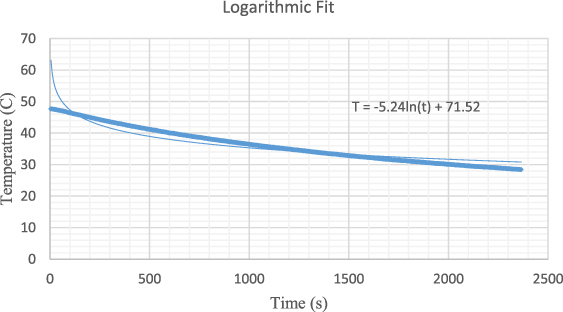
Figure 6. The temperature versus time plot managed without immersing the actual material within the water in order to justify the mathematical model. The whole range plot and the logarithmic fit with a mathematical model of T = −5.24 ln(t) + 71.52 does not demonstrate a better or perfect fit.
Download figure:
Standard image High-resolution imageAs a result, the linear fit seems to be a better way to realise the method. The other important point is that for the sake of simplicity it is legitimate to employ the linear fit rather than the log fit.
4. Results and data analysis
4.1. Results for aluminium
The experimental sequence detailed above is applied for the aluminium and the temperature is plotted as a function of time based on the data obtained by the Arduino-computer system shown in the figure 7. The temperature data, in this case, is collected by the Arduino-sensor system within every 5 s.
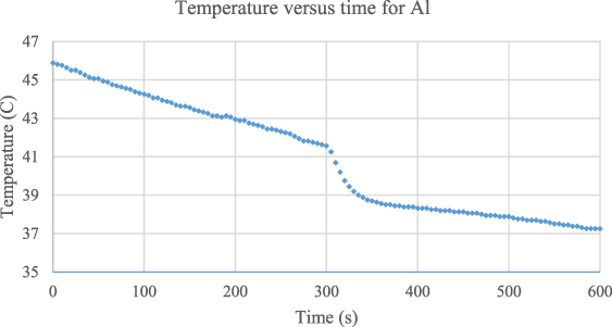
Figure 7. Temperature plotted as a function of time for aluminium, showing a clear sharp decrease due to the heat transfer from the hot water to the cold aluminium sampling.
Download figure:
Standard image High-resolution imageIt is clear from the figure that the instantaneous temperature at which the aluminium pieces are immersed within the hot water is  and corresponding time is
  . The initial temperature of the aluminium substance is separately determined and measured by a thermometer as
  . The crucial stage of the approach is the determination of the real equilibrium temperature of the water- aluminium system. This is managed by determining the temperature at which the heat transfer from the hot water to the aluminium substance is terminated. This temperature can be determined by estimating the starting point of the linear relation at the end of the sharp decrease of the temperature. The plot leads to the result that the equilibrium is reached at a temperature of
  at an instant of
  .
.
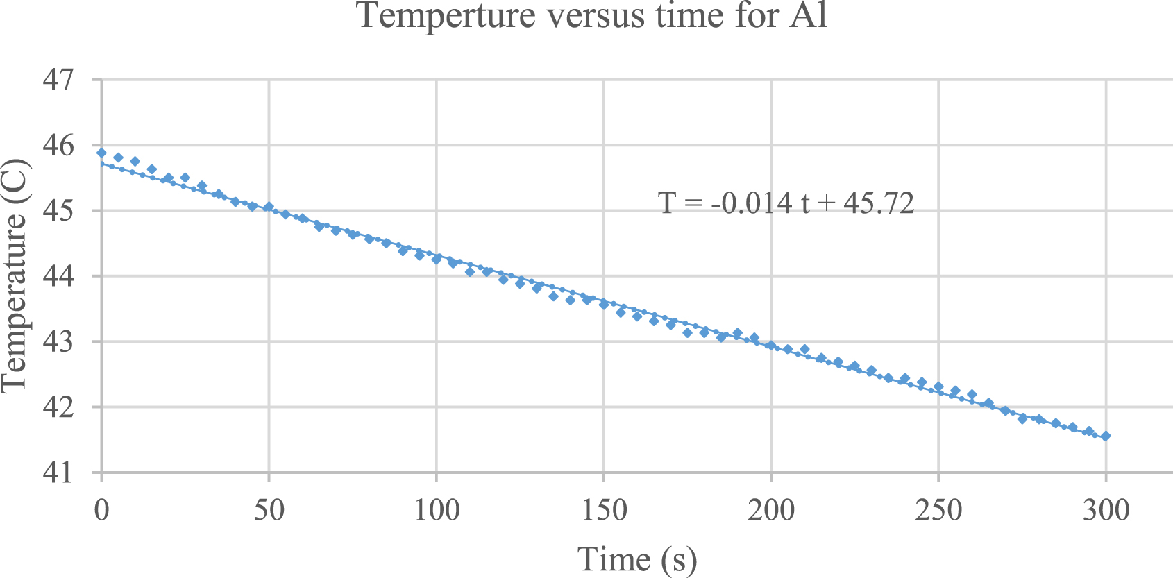
In order to eliminate the actual heat loss from the hot water container system to the environment, one ought to mathematically model the linear decrease of temperature as a function of time. This can be achieved by only taking the first linear part of the graph, that is between the temperatures of 45.88 °C and 41.81 °C, before the aluminium sampling is immersed to the hot water. The graph employed to eliminate the heat leakage/loss is shown in figure 8.
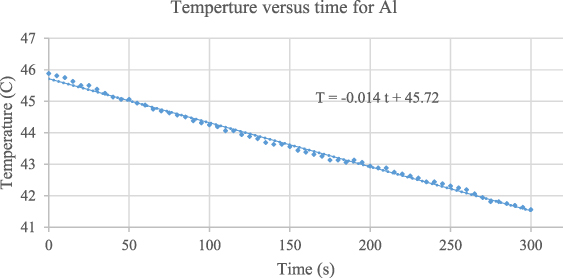
Figure 8. Time-dependent temperature graph for aluminium between the temperatures of 45.88 °C and 41.81 °C. The gradual decrease is curve fitted and mathematical modelling is found as T = − 0.014 t + 45.72.
Download figure:
Standard image High-resolution imageIt is now clear from the figure 8 that the slope of the gradual decrease of the temperature, which gives the heat loss from the hot water-container system, is determined as  based on the equation of T = − 0,014 t + 45,72. It is also possible to determine the time interval of heat transfer from the hot water and the aluminium sampling which can directly be read from the graph as
  . Accordingly, the real equilibrium temperature can be calculated as
  . The masses of the aluminium sampling and the hot water are measured five times and the average values are found to be
  and
and  , respectively. The specific heat for aluminium can now be calculated by the equation given previously as,
  . The accepted specific heat value is
  , so the relative error for this measurement can be estimated as
  , that means % 1.38 which is surely very small.
4.2. Results for copper
The same experimental structure applied for copper and the temperature is plotted as a function of time in the figure 9.
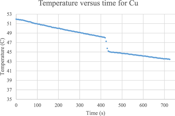
Figure 9. Temperature plotted as a function of time for copper, showing a clear sharp decrease due to the heat transfer from the hot water to the cold copper sampling.
Download figure:
Standard image High-resolution imageThis figure clearly shows that the temperature at which the copper pieces are dipped within the hot water which is read from the graph as  , and the corresponding instantaneous time is approximately
  The initial temperature of the copper is separately determined and measured by a thermometer as
  . The crucial stage of the methodology is the determination of the real equilibrium temperature of the water-copper system by eliminating the heat leakage to the environment. This is achieved by reading the temperature at which the heat transfer from the hot water to the copper is terminated. This temperature can be determined by reading the beginning point of the linear relation after the sharp temperature decrease. The graph reveals that the equilibrium is reached at a temperature of
  at an instant of
  .
.
In order to remove the actual heat leakage from the hot water-container system one ought to mathematically model the linear reduction of the temperature as a function of time. This can be succeeded by only taking the first linear part of the graph that is between the temperatures of 51.94 °C and 49.19 °C, before the copper sampling is immersed within the hot water. The graph employed to eliminate the heat leakage is shown in the figure 10.
The figure 10 clearly demonstrates that the slope of the gradual decrease of the temperature, which provides the heat leakage for the hot water-container system, is determined as  based on the equation of T = − 0.0167 t + 52.11. It is also possible to determine the time interval of the heat transfer from the hot water and the copper sampling which can directly be measured from the graph as
  . Consequently, the real equilibrium temperature can be calculated as
  . In order to determine the masses of the water and the copper, five separate measurement are carried out and the average masses are found to be,
  and
and  , respectively. The specific heat for copper can now be calculated by using the equation (10) as,
  . The accepted specific heat value for copper is
  , hence the corresponding relative error for this measurement can be estimated as
  , which means % 6.5 that is acceptable within the limits of experimental equipment.

Figure 10. Time-dependent temperature graph for copper between the temperatures of 51.94 °C and 49.19 °C. The gradual decrease is curve fitted and mathematical modelling is found to be T = − 0.0167 t + 52.11.
Download figure:
Standard image High-resolution image
5. Conclusions
In this work, a novel method is developed and reported to measure the specific heat of materials by means of a non-isolating container and an Arduino microprocessor. The method is especially significant in the sense that the specific heat measurements can be managed by means of any container without needing an isolating container. It is obvious that the method would even be more effective if an insulating container was employed. The data collections are simply accomplished by immersing the substances within the hot water and by monitoring the temperature as a function of time by means of Arduino microprocessors. This approach is mainly based on mathematically modelling the heat leakage/loss of the container-water system to the environment and eliminating that heat loss by a basic formulation. The actual measurements, managed for copper and aluminium, have exposed that the relative errors for the measurements are % 1.38 for aluminium and % 6.50 for copper. This simple approach is surely very practical, inexpensive, very easy to apply and can potentially be applied within physics or science classes. The novel method has also great potentials on scientific and engineering research undertakings and also for industrial applications.
Data availability statement
All data that support the findings of this study are included within the article (and any supplementary files).