
Abstract
An essential goal of teaching experimental physics is to engage students in exploring the validity of models and refining them. To comprehend, test, and revise scientific models, students need well-designed learning activities that enable them to practice the necessary skills. In this paper, we critically review the prevalent assumption in contemporary literature that the coefficient of kinetic friction can be treated as a constant for a certain surface pair. Further, we introduce a novel approach for calculating gravitational acceleration by measuring accelerations on inclined planes. The study indicates that kinetic friction changes with different inclinations of the plane and cannot be assumed to be constant even with typical classroom laboratory equipment. Measuring the gravitational acceleration (g) via inclined planes can result in significant deviations if varying kinetic friction is not considered. This paper proposes a lab activity to investigate the validity of a naïve friction model, by measuring the well-defined gravitational acceleration (g) with controlled precision, in an upper secondary classroom setting.
Export citation and abstract BibTeX RIS

Original content from this work may be used under the terms of the Creative Commons Attribution 4.0 license. Any further distribution of this work must maintain attribution to the author(s) and the title of the work, journal citation and DOI.
1. Introduction
Learning classical mechanics in school typically involves experimental activities to investigate and verify models related to determining gravitational acceleration and friction. Although these phenomena are interconnected, their relationship is seldom elucidated in laboratory exercises.
Modern, readily available technology opens up the possibility of analysing linear motion to study friction in numerous ways, as is evident by the resurgence of proposals for new experiments [1–12]. These include investigations of static friction [4], kinetic friction on horizontal surfaces [9, 12] and inclined planes [1, 3, 5–8]. However, a commonality among these studies is the assumption of a non-varying coefficient of kinetic friction (CoF). This shortcoming is particularly noteworthy since engaging students in refining models can be vital to their education [13].
In upper-secondary school physics, it is common when modelling friction to employ Coulomb's law,

where µ represents the coefficient of friction and  represents the normal force. In Coulomb's model (1), µ represents either the coefficient of static friction (
 ) or CoF (
 ). Without giving further thought to what µ potentially depends on, the formulation of friction as in equation (1) presents a naïve and static view of the phenomenon. It is in stark contrast to the complex and nuanced understanding of friction found in the scientific literature [14–16].
This paper introduces an innovative approach to classical upper-secondary school laboratory activities involving kinetic friction [8–11] allowing students to examine gravitational acceleration and kinetic friction. The activity offers a chance to discuss Coulomb's law of friction and its limitations without relying on additional tools such as computer modelling software [17].
2. Theoretical model
In linear motion, when an object with a sufficiently low velocity is decelerating on a horizontal surface, the net force is well approximated by friction alone (figure 1). From Newton's second law, we get

where m is the mass of the sliding object,  the tangential acceleration on the horizontal surface,
  the CoF, and g the gravitational acceleration. From equation (2), acceleration or CoF is given by

Figure 1. An object sliding on a horizontal plane (a) with velocity v is decelerated by the frictional force. The free-body diagram of the situation (b) shows that the sum of forces is zero in the y-direction and that the resulting force is equal to the friction force in the x-direction.
Download figure:
Standard image High-resolution image

and
respectively.
Constructing an inclined plane using the same surface placed at an angle θ, the resulting force on a sliding block is given by

with aθ
being the resulting acceleration of the block (figure 2). From (4),  can thus be obtained as
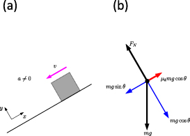
Figure 2. An object with velocity v accelerates down an inclined plane. The free body diagram (b) shows the relevant forces (black and red arrows) acting on the object when the inclination angle of the plane is θ. In addition, components of mg in the x- and y-direction are added (blue).
Download figure:
Standard image High-resolution imageHowever, equation (5) assumes that the gravitational acceleration g is known. By substituting equation (3a ) in (4) and solving for g, we arrive at
3. Method
3.1. Materials
- Smartphone
- Built-in camera
- Phyphox (inclination tool) [18]
- Tracker [19]
- PVC object (57 mm diameter disk)
- Aluminium (58 mm diameter, muffin cup)
- Table surfaces (laminated and raw plywood)
- Ruler.
3.2. Data collection
To calculate g using equation (6) two accelerations ( and aθ
) and the inclination angle (θ) had to be measured. A ruler was attached to a table surface and an object was placed near the ruler. For
and aθ
) and the inclination angle (θ) had to be measured. A ruler was attached to a table surface and an object was placed near the ruler. For  , the object was given an initial impulse by hand with
  ; for aθ
, the object was released with the surface tilted at an angle θ > 0, such that sliding occurred. A smartphone camera was used to record the events.
; for aθ
, the object was released with the surface tilted at an angle θ > 0, such that sliding occurred. A smartphone camera was used to record the events.
The inclination angle of the plane was measured using Phyphox inclination tool, by placing the smartphone on the inclined surface (figure 3(a)). The smartphone camera was aligned at the same angle as the plane before recording the sliding motion. This ensured that the sliding motion was recorded without distorting the path travelled by the object.
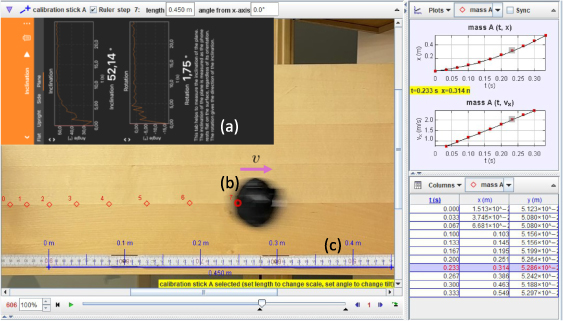
Figure 3. An object sliding down the inclined plane, analysed in Tracker. The inset (a) is the Phyphox inclination tool from the smartphone mounted at the same angle as the plywood surface. The sharp back contour of the moving object is tracked using the autotracker in Tracker (b). A calibration stick in Tracker was aligned with the ruler in the video to calibrate distance (c).
Download figure:
Standard image High-resolution imagePer recommendations in Tracker, the camera recorded at 1080p, 30 frames per second. One effect of using this framerate is a noticeable motion blur of the sliding object as the velocity increases. A point towards the rear of the sliding object (figure 3(b)) was used to track the path travelled to reduce the error induced by motion blur. The uncertainty in object position in each frame was estimated to be ±3 pixels. Finally, the ruler in the video was used to calibrate the length scale when analysing the motion in Tracker (figure 3(c)). The estimated relative error for the calibration was ±0.1 .
.
The two accelerations  and aθ
in equation (6) were obtained by auto-fitting a linear model to the
and aθ
in equation (6) were obtained by auto-fitting a linear model to the  -graphs in Tracker's data tool. The gravitational acceleration and CoF were then calculated by equations (6) and (3b
) within the model. For reference,
-graphs in Tracker's data tool. The gravitational acceleration and CoF were then calculated by equations (6) and (3b
) within the model. For reference,  was also calculated by the use of equation (5), with
  [20].
[20].
4. Results
The experiment quantified the gravitational acceleration g, for two different surface pairs. The data showed that the value of g fluctuated with changes in the inclination angle (figure 4). CoF was determined using the calculated g value and compared (figure 5) to calculations using the standard gravitational acceleration value of 9.81 m s−2, commonly referenced in typical textbooks. Each point represents the average of several measurements (20 for PVC and 5 for aluminium) and the error bars' length represents one standard deviation.

Figure 4. Angle-dependent variations of g for two different surface pairs: PVC sliding on raw plywood (red dots) and aluminium sliding on a laminated table surface (black diamonds). Each point represents the average of several measurements (20 for PVC and 5 for aluminium) and the error bars' length represents one standard deviation. The blue dashed line indicates the textbook value of g.
Download figure:
Standard image High-resolution image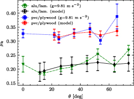
Figure 5. Angle-dependent variations of CoF for the two different surface pairs (PVC sliding on raw plywood (blue and red) and aluminium sliding on a laminated table surface (green and black)), using g = 9.81 m s−2 and the g calculated using equation (6).
Download figure:
Standard image High-resolution image5. Discussion
This study describes a method that can be implemented as a lab exercise in an upper-secondary physics class. It involves measuring the well-defined gravitational acceleration (g) with controlled precision to test and discuss the validity of a naïve friction model.
We determined the gravitational acceleration g by using objects sliding on inclined planes. Equation (6) was used to calculate g without initially determining the coefficient of kinetic friction, CoF. However, this method produced angle-dependent results and thus large deviations in the determination of g, as shown in figure 4. The error bars did not overlap with the established value for g for some angles. In fact, for some points on the investigated surfaces, the interval within the error was above the known value for g (9.81 m s−2), while for other points, it was below. Herein lies the strength of the proposed procedure. Students can recognise something is wrong with the underlying assumptions since they know what value g should get in a measurement.
The measured values of g appear to vary depending on the angle. Similarly, other basic parameters, such as normal force and object speed, which have been shown to have a weak influence on CoF [15], also vary with angle. The experiments were performed with inclination angles above the critical angle for static friction. Still, the larger deviation from g at small angles might be attributed to effects stemming from the transition from static to kinetic friction, such as minuscule stick-slip motion [21]. To amplify the angle-dependent effects, a stainless steel object sliding on a stainless steel surface can be used [22].
In the next step, the obtained values for the gravitational acceleration can be used to calculate CoF by equation (3b
). However, then  is used once more, and only subtle variations in CoF are observed, with error bars that do overlap (red dots and black diamonds in figure 5). We did a comparison of these values for CoF to the true CoF variations using the standard gravitational acceleration, as seen in figure 5. The method transferred some of the variations in CoF to variations in g. The error bars for the true CoF exhibit larger variations. Additionally, the error bars mostly overlap (blue squares and green triangles in figure 5), making it insufficient to test assumptions about a constant CoF.
Similar to the experiment presented in this paper and other works [9, 11], an underlying assumption when working with naïve models of friction is that CoF must not vary with angle. Nevertheless, as we have shown (figure 4), in a way comprehensible for students, by measuring g, this is not the case. Angle-dependent variations of CoF occur for several surfaces. Further, these variations in CoF are present, yet uncommented, in previous studies with an educational focus [3, 5, 6]. However, as indicated by the current study and earlier work [1], it is possible, using typical classroom laboratory equipment, to study the complex nature of CoF.
The procedure described in this article only requires two accelerations:  and aθ
. There are multiple ways to experimentally obtain them in a classroom. A complementary attempt to use accelerometer sensor data instead of the camera with the Tracker software was made with similar results. However, extracting data via Tracker rather than downloading the sensor data from an app may offer benefits for novice physics learners at the upper-secondary level, aiding in the correlation of various concepts visualised within the Tracker environment. The use of a sensor app also requires skills in handling data in either spreadsheets or by programming. However, the latter method is more closely aligned with the practices of physics researchers, and therefore each method holds value at different stages of a student's model refinement process.
and aθ
. There are multiple ways to experimentally obtain them in a classroom. A complementary attempt to use accelerometer sensor data instead of the camera with the Tracker software was made with similar results. However, extracting data via Tracker rather than downloading the sensor data from an app may offer benefits for novice physics learners at the upper-secondary level, aiding in the correlation of various concepts visualised within the Tracker environment. The use of a sensor app also requires skills in handling data in either spreadsheets or by programming. However, the latter method is more closely aligned with the practices of physics researchers, and therefore each method holds value at different stages of a student's model refinement process.
To exemplify a meaningful learning situation, one might employ the procedure for a single angle, along with 0∘ (see figures 6 and 7, respectively). From this, we get that the average  and
and  (table 1). The measurement has high precision but provides evidence of a gravitational acceleration outside the expected value.
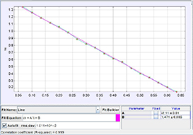
Figure 6. Example data collection from a sliding aluminium muffin cup decelerating on a horizontal laminated table. The acceleration is obtained as the slope of a linear model fitted to the  -graph using Trackers' data tool. The fitted function is
  .
.
Download figure:
Standard image High-resolution image
Figure 7. The aluminium muffin cup accelerates down a tilted laminated table at 52.1∘ inclination. The acceleration is obtained by the auto-fit of a linear model to the  -graph, using the Tracker data tool. The fitted function is
  .
.
Download figure:
Standard image High-resolution image
Table 1. Results from a sliding aluminium muffin cup decelerating on a laminated table tilted at 52.1∘ angle. The left column holds values from measurements and calculations and the right column the corresponding uncertainty. The values are the average of five measurements. The uncertainty is given as one standard deviation (rounded up) of the data for θ,  , and aθ
. The uncertainty of g and
, and aθ
. The uncertainty of g and  is calculated with error propagation.
| Value | Uncertainty | |
|---|---|---|
| θ | 52.1∘ | 0.5∘ |

| 2.13 m s−2 | 0.27 m s−2 |
| aθ | 6.21 m s−2 | 0.11 m s−2 |
| g | 9.53 m s−2 | 0.25 m s−2 |

| 0.22 | 0.03 |
We encourage teachers to activate students in a collaborative data collection process where lab groups collect data at different angles. This can lead to results similar to those in figure 4 during a single lab session. From this, teachers can initiate students in a discussion about how it is crucial to examine assumptions about the underlying models upon which physics experiments are based.
Our results imply that investigating CoF alone will be insufficient for students' naïve models of CoF to be challenged. This would require even more precise measurements or manipulation of necessary parameters to increase the effects shown in figure 5. Instead, with the proposed method we designed a learning activity for students to measure g without first determining CoF, as exemplified above. This will provide students with an opportunity to test any held assumptions of a constant CoF. Thereafter, teachers can help them to initiate further work revising their models. Although this activity remains to be implemented fully in practice, the design provides a novel possibility for testing, revising, and discussing models of kinetic friction in upper-secondary physics classrooms while conducting gravitational acceleration measurements.
6. Conclusion
A novel take on a classic laboratory activity has been developed to challenge a simplistic view of kinetic friction among upper-secondary school students. Precise measurements of the gravitational acceleration g were introduced using sliding objects on an inclined plane. The data for the acceleration down an inclined plane and the corresponding deceleration on a horizontal plane were extracted to calculate the acceleration due to gravity (g) and the CoF. The main results indicate g to be dependent on the angle of inclination during sliding experiments on two different pairs of surfaces. This is used to challenge a simplistic view of the friction concept since the calculated variations in g must stem from a non-constant CoF. Further research is necessary to explore upper-secondary school students' learning experiences as they experiment with models and their assumptions in classical mechanics. The approach described here aims to inspire both teachers and students to investigate their own models of kinetic friction.
Acknowledgments
Andreas: conceptualisation; formal analysis; investigation; methodology; visualisation; writing—original draft; writing—review & editing (equal).
Sebastian: formal analysis (supporting); writing—original draft (supporting); writing—review & editing (equal).
Jonas: supervision; writing—review & editing (equal).
Data availability statement
The data cannot be made publicly available upon publication because they are not available in a format that is sufficiently accessible or reusable by other researchers. The data that support the findings of this study are available upon reasonable request from the authors.
Biographies

Andreas Johanson is a PhD student in physics education research at the Department of Physics at the University of Gothenburg. His research interests include student learning processes in laboratory settings and laboratory development. He has a background as a high school physics and mathematics teacher.

Sebastian Kilde Löfgren is a PhD student in physics education research at the Department of Physics at the University of Gothenburg. His research interests include student learning processes in laboratory settings with a focus on model development and modeling. He has a background as a high school physics and mathematics teacher.

Jonas Enger is an assistant professor in physics at the Department of Physics at the University of Gothenburg. His research interests include student learning processes in high school physics. He has a background as a high school principal and as a high school physics and mathematics teacher.