

Abstract
A more inclusive and detailed measurement of various physical interactions is enabled by the advance of high-speed data digitization. For surface potential characterization, this was demonstrated recently in terms of open-loop amplitude modulation Kelvin probe force microscopy (OL AM-KPFM). Its counterpart, namely open-loop frequency modulation Kelvin probe force microscopy (OL FM-KPFM), is examined here across different materials and under various bias voltages in the form of OL sideband FM-KPFM. In this implementation the changes in the amplitude and resonance frequency of the cantilever were continuously tracked as a conductive AFM probe was modulated by a 2 kHz AC bias voltage around the first eigenmode frequency of the cantilever. The contact potential difference (CPD) between the AFM probe and sample was determined from the time series analysis of the high-speed 4 MHz digitized amplitude and frequency signals of the OL sideband FM-KPFM mode. This interpretation is demonstrated to be superior to the analysis of the parabolic bias dependent response, which is more commonly used to extract the CPD in OL KPFM modes. The measured OL sideband FM-KPFM amplitude and frequency responses are directly related to the electrostatic force and force-gradient between the AFM probe and sample, respectively. As a result, clear distinction was observed for the determined CPD in each of these cases across materials of different surface potentials, with far superior spatial resolution when the force-gradient detection was used. In addition, the CPD values obtained from OL sideband FM-KPFM amplitude and frequency measurements perfectly matched those determined from their closed-loop AM-KPFM and FM-KPFM counterparts, respectively.
Export citation and abstract BibTeX RIS
1. Introduction
Kelvin probe force microscopy (KPFM) is an atomic force microscopy (AFM) mode in which the contact potential difference (CPD) between a conductive AFM probe and a sample is extracted by observing the electrostatic interaction between probe and sample at the nanoscale level. It was introduced by Nonnenmacher et al [1] in 1991 and, to some extent, resembles Lord Kelvin's observation of electric flow between two materials of different surface potential that are brought into contact. The most common versions of KPFM are in the forms of amplitude-modulation KPFM (AM-KPFM) [1, 2] and frequency-modulation KPFM (FM-KPFM) [3, 4]. Routinely, these KPFM modes are implemented on commercial AFMs as closed-loop (CL) procedures, seeking to determine the local CPD between an AFM probe and the investigated sample by nullifying either the electrostatic force (CL AM-KPFM) or the gradient of the electrostatic force (CL FM-KPFM) between the probe and sample [5]. Over years, these implementations became some of the most used AFM imaging modes for electric surface property characterization through the plethora of probe-sample interactions that are either directly or indirectly extracted from CPD measurements across a large variety of materials and structures including metals [1, 6], semiconductors [3, 7], dielectrics [8, 9], photovoltaics [10, 11], polymers [12–14], ferroelectrics [15–17], and biological samples [18–20]. A comprehensive coverage of various KPFM instrumentation aspects and applications for nanoscale material property characterization can be found in review articles [14, 21–23].
In recent years, significant developments were made to capture the fast response of the tip-sample electrostatic interaction in the time domain [11, 24–27]. A faster and more inclusive measurement of this interaction would provide the KPFM-type output, namely the CPD, on a shorter time scale capable of observing more details of various nanoscale electrodynamic processes, which otherwise are masked in KPFM measurements made in the frequency domain. Some of these developments aim towards open-loop (OL) KPFM modes with high-speed data capture of the cantilever response. Notably, ultrafast OL implementations like time-resolved electrostatic force microscopy (EFM) [24, 25], pump-probe KPFM [26, 27], and fast free force recovery KPFM [28] were successfully used to examine the dynamics of the optoelectronic response of materials and electric field-induced charge migration for time scales on the order of tens of microseconds.
In this work the high-speed digitization of the OL sideband FM-KPFM amplitude and frequency signals is analyzed on materials of various surface potentials and under different bias voltages. It is the purpose of this study to examine the differences between force (given by amplitude) and force-gradient (given by frequency) responses of the OL sideband FM-KPFM mode and compare them to those from the more established CL configurations of the KPFM, namely AM-KPFM and FM-KPFM. In this implemented OL sideband FM-KPFM the deflection and resonance frequency of a conductive AFM probe are sampled at 4 MHz rate while the electrostatic tip-sample interaction is modulated by a 2 kHz bias voltage in the lift mode of a peak-force tapping scan. The high-speed data capture allows a time series analysis of the amplitude and frequency signals for the extraction of the CPD values. Notably, the CPD determined from OL sideband FM-KPFM frequency measurements shows greater spatial resolution and is less sensitive to the variability introduced by the weighted averaging of various stray capacitive couplings between the AFM cantilever and the heterogeneous regions of the sample than the CPD obtained from OL sideband FM-KPFM amplitude measurements. This is because, on one hand, the CPD determined from the frequency response of the OL FM-KPFM shows tip-confined resolution in much the same way as that provided by CL FM-KPFM as both measurements stem from the force-gradient interaction between tip and sample. On the other hand, the CPD values determined from the amplitude of OL sideband FM-KPFM match those obtained from CL AM-KPFM as both types of measurements derive from the AFM probe-sample force response.
2. Amplitude versus frequency modulation in KPFM
The basic functionality of various KPFM implementations resides on the electrostatic interaction between a conductive AFM probe and sample. To express this electrostatic interaction, quite common in KPFM, is to use a combination of a DC voltage,  , and an AC voltage,
  applied either on the AFM probe or sample, in the form of a bias voltage,
  . Under this bias, the AFM probe-sample electrostatic force,
  , includes the CPD voltage that is to be determined in KPFM as
where PS refers to the probe-sample interaction and  is the gradient of the probe-sample capacitance with respect to the probe-sample distance
  ;
;  depends on the probe-sample distance
  , probe-sample geometry, and dielectric properties of the sample and measurement environment. Simple mathematics shows that
  is made of three distinct parts, one static component,
  , and two dynamic components: One at the frequency of the AC voltage,
  , and another at the double of the frequency of the AC voltage,
  :
:
It is straightforward to observe that the z-gradient of  ,
,  , will have the same voltage dependence as
  (given by equations (1) and (2)) because the z-derivative acts only on the
  factor. In the most general form of EFM, the above equations are used to interpret various contributions to the probe-sample electrostatic interaction and, based on that, provide quantitative property characterizations of the sample. The difficulty in EFM resides on the precise modeling of the geometry of the AFM probe-sample capacitor and dielectric properties of the system, these parameters being included in the
  term [28–30]. However, KPFM simply aims to provide a direct measurement of the CPD between the AFM probe and sample, so the terms of interest are the voltage dependent contributions in equation (2), without too much interpretation of the
  part.
part.
In CL AM-KPFM [1, 2], the AC voltage is applied on either tip or sample with the frequency  usually matching the first free-resonance frequency
  of the AFM cantilever to enhance the induced deflections of the AFM probe; in some CL AM-KPFM implementations,
  is either a non-resonance or a higher eigenmode frequency of the cantilever. The frequency of this driving excitation is maintained constant and a lock-in amplifier (LIA) is used to detect the amplitude
  and phase
  of the cantilever deflections at this frequency. In the same time, a feedback-loop is adjusting continuously the
  voltage such to nullify the
  component detected by the LIA and, according to equation (2b), this will give a measurement for
  In practice, there are a series of factors like probe-sample stray capacitive couplings, probe-sample distance, topography cross-talk, as well as some cumulative feedback effects that could prevent the accurate determination of
  from CL AM-KPFM measurements [31–35].
In CL FM-KPFM [3, 4, 36], the z-gradient of the electrostatic force  is sought to be nullified by the feedback-loop instead of the electrostatic force as in CL AM-KPFM. The gradient
  directly relates to changes in the resonance frequency of the cantilever
  through the induced variations in the effective spring constant of the cantilever
where  is the cantilever spring stiffness. Furthermore, in CL sideband FM-KPFM mode [4], the electrical modulation
  (
( ) is additionally mixed with a mechanical modulation at the resonance frequency of the cantilever
  to improve the detection sensitivity. In this case, as inferred from equations (2b), (2c), and (3), the cantilever dynamics will undergo frequency modulations at
  and
and  in the form of amplitude sidebands on each side of the resonance peak. As such, the feedback-loop of the CL sideband FM-KPFM is seeking to actively nullify the sidebands at
  during the lift mode and report the
  voltage as
  . The main benefit of FM-KPFM over AM-KPFM is its enhanced spatial resolution due the faster lateral decay of the force-gradient than that of the force. Combined modeling and experiments [37, 38] showed that the force-gradient signal measured by FM-KPFM is mainly responsive to the capacitive coupling between the tip (apex and cone) and its surrounding sample and independent on the probe-sample distance. On the other hand, the force signal measured by AM-KPFM has less spatial contrast as including contributions from both tip-sample and cantilever-sample capacitive couplings and depends on the tip-sample distance [32, 39]. The difference steams mostly from the z-dependence of various constituent parts to the probe-sample capacitance,

where  is for the apex-sample capacitance,
  is for the truncated cone sample capacitance, and
  is for the cantilever-sample capacitance. It has been shown [40] that, for probe-sample separations
  much smaller than the tip height,
  is almost independent of
  , which makes the FM-KPFM signal less sensitive to the contribution from the cantilever-sample capacitive coupling. Therefore, the cantilever contribution can significantly alter the
  reported by AM-KPFM but has little influence on the
  measured by FM-KPFM [37, 38]. Besides the spatial averaging response that is characteristic to each method, in both AM-KPFM and FM-KPFM operated in CL, the reported
  value at each pixel in the scan reflects an average value over a time scale commensurable with the time constant of the feedback-loop, which could be around 1 ms in some implementations.
The incentive to reduce the artifacts associated with the CL bias feedback, measure voltage sensitive materials, and enable the observation of fast electrodynamic processes stimulated in the last years the investigation of various open loop implementations of KPFM, namely to operate KPFM without using  as a feedback parameter. One of the proposed OL AM-KPFM methods was to simultaneously measure the first two harmonic amplitudes,
  and
and  provided by equations (2b) and (2c). For a given
  , with
  , the ratio of the two amplitudes provides quantitative measurements for
  if the cantilever transfer function gain is known. The method is known as the dual harmonic (DH) KPFM [35] and has been shown to work well on voltage sensitive materials [41] and solid-liquid interfaces [42, 43] where regular AM-KPFM does not perform very well.
Another OL AM-KPFM method was proposed with a high-speed digitization of the cantilever deflection that recovers the bias dependence of the probe-sample electrostatic force under the drive of the  (
( ). The method was called general acquisition mode (G-mode) KPFM [44–46] and uses sampling rates of order of MHz and AC bias voltages with frequencies up to tens of kHz to increase the spatial and temporal resolutions of the measurements. Pertinent for the interpretation of these OL measurements is to highlight the parabolic bias dependence of equation (1)

where  has only an AC part and
  is determined from the location of the apex of the parabola,
  . With the fast digitization, G-mode KPFM recovers the parabolic dependence of the electrostatic force during each of the AC cycles by low-pass filtering the acquired cantilever deflection [28, 45–47]. The CPD response of the G-mode KPFM is on a time scale as short as 20 μs [27, 46], which is about one hundred times faster than in common CL KPFM modes and allows observation of ultrafast dynamics of electrical processes [28]. Although open-loop, OL AM-KPFM methods determine the
  from the measured amplitudes, which means that non-local contributions from the cantilever will still be present. In the following, the high-speed digitization will be examined for both amplitude and frequency measurements in OL sideband FM-KPFM on a test sample showing regions of distinct surface potentials. By comparing the results from these OL sideband FM-KPFM measurements to those from CL AM-KPFM and CL sideband FM-KPFM, the force versus force-gradient paradigm of KPFM mode is addressed here in the context of the OL implementations of this technique.
3. Materials and measurement methods
The experimental setup used for the high-speed measurements was implemented on the PeakForce FM-KPFM mode [48] of a MultiMode 8 Bruker AFM (Bruker Nano Surfaces, Santa Barbara, CA, USA) with each scan line performed in two passes: In the first pass (trace and retrace) the surface topography is tracked by PeakForce tapping (PFT) (refer to figure 1(a)) and in the second pass (trace and retrace in lift mode) the electrostatic response of the sample to the applied modulations is observed at some constant height above the sample surface while the tip follows the topography acquired in the first pass (refer to figures 1(b) and (c)). The scanning rate was 0.5 Hz per scan line with 512 pixels per line. The probes used were PtIr coated Si probes SCM-PIT-V2 (Bruker AFM Probes, Camarillo, CA, USA) with a nominal spring constant around 3 N m−1 and first resonance frequency  around 65 kHz. In topography, the PFT modulation was performed at 2 kHz and 50 nm amplitude. The lift height was 75 nm to minimize the short-range contributions to the probe-sample interaction. In the CL sideband FM-KPFM mode (figure 1(b)), the bias voltage feedback-loop of the KPFM is activated while the probe is mechanically oscillated at its first resonance frequency and electrically modulated at
  = 1.95 kHz and
  = 4.75 V. By using two-cascaded lock-in amplifiers, the CL of PeakForce FM-KPFM adjusts the DC bias to nullify the sidebands at
  . In all the measurements in this work the bias voltages was applied on the AFM probe and the sample was grounded, unless otherwise specified. In the following, the measurements described above will be referred to as CL sideband FM-KPFM.
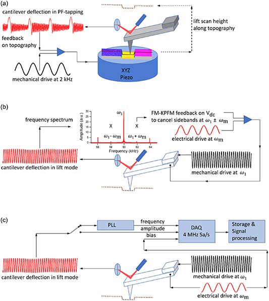
Figure 1. (a) Schematic of the peak-force tapping performed in the first pass of the CL and OL sideband FM-KPFM modes to track the topography of the sample; (b) Schematic of the lift mode performed in the second pass of CL sideband FM-KPFM where the topography acquired in (a) is followed at a given height above the surface. Concurrently with the mechanical and electrical modulations applied on the cantilever the feedback-loop is adjusting the  voltage to match the surface potential; (c) Schematic of the lift mode performed in the second pass of OL sideband FM-KPFM where no feedback on
  is engaged but, instead, either the deflection or frequency response of the cantilever is sampled at high speed, simultaneously with the electrical modulation.
Download figure:
Standard image High-resolution imageThe high-speed OL measurements were performed in the configuration shown in figure 1(c) with the bias voltage feedback-loop disengaged. In this mode, two signals, the bias voltage and either the deflection or resonance frequency of the cantilever, were recorded by a NI PCI-6111 data acquisition board (National Instruments, Austin, Texas, USA) at a rate of 4 MHz. The high-speed data collection was triggered at the beginning of the lift mode and acquired either in the trace or retrace parts of the lift mode. For OL sideband FM-KPFM amplitude measurements, the cantilever deflection was directly sampled from the signal access module of the AFM whereas for OL sideband FM-KPFM frequency measurements the cantilever deflection signal was feed through a phase-lock loop system (PLL) and the shift in the resonance frequency measured along with the bias modulation, also at 4 MHz sampling rate. The PLL used was from an UHFLI lock-in amplifier (Zurich Instruments, Zurich, Switzerland) and it was configured as an internal PLL, without applying any drive on the AFM probe but only to track the induced changes in the resonance frequency. The bandwidth of the PLL filter was increased up to 12.5 kHz to properly track the frequency response of the cantilever to the modulations used by the FM-KPFM. For completeness, AM-KPFM measurements were also done in PeakForce AM-KPFM, referred to as CL AM-KPFM, with an electrical bias at the first resonance frequency of the cantilever and 2 V amplitude. The CL PeakForce AM-KPFM mode is a two-pass scanning with topography acquired in the first pass by PeakForce tapping and CL AM-KPFM performed in the second pass at a lift height above the surface; both trace and retrace were made in each pass.
Short segments of high-speed data measurements for OL sideband KPFM are shown in figure 2 for both amplitude (figure 2(a)) and frequency (figure 2(c)) measurement configurations. Both measurements were performed above an Au region of the Au/Si/Al test PFKPFM sample (Bruker AFM Probes, Camarillo, CA, US) at locations close to each other. Both raw signals have a strong carrier oscillation at the first resonance of the cantilever (mechanical drive)  but also include a low-frequency modulation. The frequency components of these modulations are displayed by the fast Fourier transform (FFT) amplitude spectra of the signals, in figure 2(b) for amplitude and in figure 2(d) for frequency shift. In both cases, strong peaks are observed at
  and
and  as well as at the modulation frequency
  and its harmonics, both at low frequency and around the driving frequency,
  and its double
  ; modulation are also present at higher harmonics of
  . The response conveyed by the envelope modulation can be easily retrieved by applying a low-pass frequency filter to retain only the low frequency components. The filter was a finite impulse response Blackman filter from IgorPro (WaveMetrics, Lake Oswego, OR, USA) with end of pass band at 10 kHz and start of reject band at 15 kHz. As is shown in the FFT of the filtered signals (figures 2(b) and (d)), all the high-frequency content above 15 kHz is removed and the filtered signals (figures 2(a) and (c)) resemble the modulated envelopes of the measured signals. Alternatively, the separation of the electrostatic response from the mechanical dynamics of the cantilever can be done by deconvoluting the transfer function of the cantilever from the FFT spectra of the measured signals [28].

Figure 2. (a) Raw (orange) and filtered (black) cantilever deflection signals from high-speed OL sideband FM-KPFM amplitude; (b) FFT of the raw (orange) and filtered (black) signals shown in (a); (c) raw (light blue) and filtered (dark blue) of the frequency shift signals from high-speed OL sideband FM-KPFM; (d) FFT of the raw (light blue) and filtered (dark blue) of the signals shown in (c).
Download figure:
Standard image High-resolution image4. Results and discussion
Besides the common analysis of the parabolic bias-dependence of the KPFM response given by equation (5), either in amplitude or frequency, another way of looking at this in high-speed measurements is to consider the time-dependence of the response. This is to fit the response functions (filtered amplitude or frequency signals) to

where  ,
,  ,
,  , and
, and  are fit parameters and
  and
and  are fixed parameters,
  = 4.75 V and
  = 1.95 kHz in this work. In equation (6) the variable is
  whereas in equation (5) the variable is
  . The
. The  parameter is to consider possible voltage offsets and baseline adjustment after signal conditioning. The
  parameter is proportional to the capacitive gradient specified by equation (1) but its physical meaning and content of information (e.g. for dielectric characterization) will not be further detailed in this study. Regarding the
  used, it should be mentioned that the nominal value of
  as the applied bias on the tip was 5.0 V in the AFM settings but measured as 4.75 V, the 5% difference being related to possible internal offsets of the instrument; 4.75 V was the actual applied bias on the tip. In figures 3(a) and (c) are shown two amplitude sequences of three consecutive bias periods over the Au and Al regions of the sample, respectively. For the middle period, each of these signals was fitted by equation (6) with 0.09 V and 0.83 V for the fit parameter
  on Au and Al, respectively. The variations for
  as determined from the time series analysis given by equation (6) were not more than 5 mV from period to period whereas the parabolic fit (equation (5)) showed variability around 50 mV within each bias period and from period to period. In figure 3(b) are shown two such parabolic fits for the regions marked in figure 3(a) as R1 (bias going from positive to negative voltages) and R2 (bias going from negative to positive voltages) but in terms of amplitude versus bias as used in equation (5). Similarly, in figure 3(d) are shown the parabolic bias fits for the regions marked as R3 and R4 in figure 3(c). The reason why the temporal fit (equation (6)) performs better than the parabolic fit (equation (5)) is that the entire oscillation is followed in the temporal fit, including the response around maximum, minimum, as well as around zero bias voltages whereas only the region around zero bias is probed by the parabolic fit. The results for
  from parabolic fits are considerable improved at higher frequency modulations when many values are determined and averaged over each scan location [28, 46]. It should be also noted the characteristic response of the amplitude-modulated time series for small and large values of
  . At small values of
  (refer to figure 3(a)) there is a negligible change in the magnitude of the oscillation's amplitude between the side with positive bias gradient (bias increasing from
  to
to  ) and the side with negative bias gradient (bias decreasing from
  to
to  ); as shown by equation (6) there will be no shift when
  = 0 V. However, at large values of
  (refer to figure 3(c)) there is a significant change in the magnitude of the amplitude from one side to another of the oscillation's amplitude. This is because
  is not changing the sign and has a different contribution to the negative and positive bias ramps.

Figure 3. (a) Sequence of low-pas filtered amplitude time series over three consecutive bias periods over the Au region of the sample (the amplitude signal is assigned to the left axis and bias signal to the right axis); (b) Parabolic dependence of the measured amplitude versus bias voltage within the regions R1 and R2 marked in (a); (c) Sequence of low-pass filtered amplitude time series over three consecutive bias periods over the Al region of the sample (the amplitude signal is assigned to the left axis and bias signal to the right axis); (d) Parabolic dependence of the measured amplitude versus bias voltage within the regions R3 and R4 marked in (c). The thicker dashed lines in (a) and (c) over the central period are fits of the amplitude versus time given by equation (6) (see text for details).
Download figure:
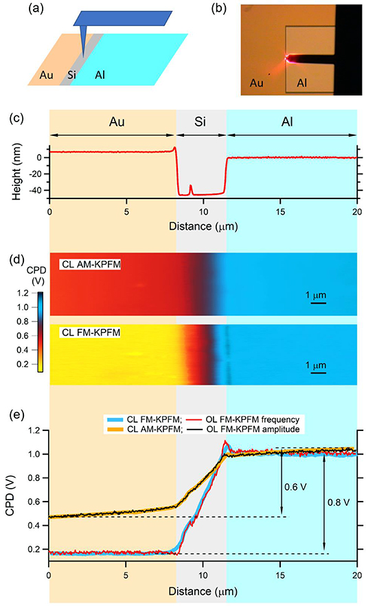
Standard image High-resolution imageSimilarly, the time series analysis described by equation (6) can be applied to OL sideband FM-KPFM frequency measurements. In figure 4, results from high-speed OL sideband FM-KPFM amplitude and frequency measurements are compared side by side over one of the Au/Si/Al trenches of the sample. For reference, the values of  from CL AM-KPFM and CL sideband FM-KPFM scan lines across the same trench are also plotted. While the four types of measurements were not done simultaneously over the exact locations, the scan lines were performed within few micrometers from each other and are representative for the values and trends of each method. The scan lines discussed in figure 4 were over 20 micrometers in length covering about 7.5 micrometers of Al and Au regions on each side of the Si trench. As is shown in figures 4(a) and (b), the AFM cantilever was almost entirely hovering over the Au part during scanning. The position of the cantilever with respect to the scanned area will be carefully noted in the following due to its relevance to the AM-KPFM results. For both OL sideband FM-KPFM amplitude and frequency modes, a scan line consists of about 488 points, the value at each point being the average of
  values obtained from 4 consecutive bias oscillations (1950 oscillations per line/4
  488 pixels per line); the period of the bias oscillation was 512 μs. The measured frequency shifts were with respect to the frequency locked by PLL, which was very close to but not necessarily the exact free-resonance frequency of the cantilever.

Figure 4. (a) Schematic and (b) picture from above of the AFM probe (tip + cantilever) during scanning over the Al/Si/Au trench. (c) Traces of CPD from CL AM-KPFM, CL sideband FM-KPFM, and OL sideband FM-KPFM amplitude and frequency scan lines over the Al/Si/Au trench. (d) and (e) Time series of the bias modulation and low-pass filtered OL sideband FM-KPFM amplitude and frequency shift over Al and Au, respectively. The central modulation period was fitted by equation (6) (see text for details).
Download figure:
Standard image High-resolution imageAs can be seen in figure 4(c), very good agreement was obtained between the  values determine from CL AM-KPFM and OL sideband FM-KPFM amplitude modes on one hand and CL sideband FM-KPFM and OL sideband FM-KPFM frequency modes on the other hand across every region of the sample: Au, Si, and Al. The main observation here is that the
  values determined from OL sideband FM-KPFM frequency and CL sideband FM-KPFM modes account for a CPD of about 0.8 eV between Al and Au, whereas those determined from OL sideband FM-KPFM amplitude and CL AM-KPFM modes make only about 0.6 eV difference in the surface potentials of these two metals. In addition to that, both amplitude-based measurements (CL AM-KPFM and OL sideband FM-KPFM amplitude modes) show a broader transition at the Al/Si and Si/Al interfaces than their frequency-based (CL sideband FM-KPFM and OL sideband FM-KPFM frequency modes) counterparts. While it might be tempting to qualify AM-KPFM as less sensitive than FM-KPFM, the above observations are direct evidence of the cantilever-sample capacitance contribution to the electrostatic force measured by AM-KPFM. As discussed above, the gradient-type measurement implied by FM-KPFM significantly minimizes this cantilever-sample coupling and provides a more accurate measurement for the tip-sample CPD. Indeed, from figure 4(c) it is clearly observed that the measurement accuracy of the AM-KPFM mode is altered only over the Si and Al parts that are not directly overlooked by the cantilever during scanning. In this case, there is a heterogeneity in the sample-cantilever stray capacitance due to the difference in the CPD between the cantilever and the scanned region (Si or Al) and CPD between the cantilever and the sample underneath (Au in this case). As it was detailed in previous works [38], these sample heterogeneities are convoluted into the weighted average of the CPD reported by AM-KPFM. On the other hand, when the AFM probe scans over the Au part, where the cantilever resides, both the AM and FM modes (either OL and CL) provide the same weighted average of the CPD because in this case the CPD variability introduced by various regions of the sample to the stray capacitances, sample-probe and sample-cantilever, is minimum, i.e. the scanned area and its surroundings show low heterogeneity in terms of surface potential. The results discussed here correlate with previous reports on the difference in the CPD determined from electrostatic force and force gradient detection of the OL band-excitation KPFM: It has been observed that the CPD of an Au strip deposited on a Si substrate is about 465 mV smaller when measured by force than force gradient, most likely due to the stray capacitance contributions from the non-local electrostatic couplings between the AFM probe and sample [49].
In figures 4(d) and (e) are shown short time series of the low-pass filtered signals of the OL sideband FM-KPFM amplitude and frequency measurements on Al and Au, respectively. Both types of signals are very well fitted by the time-dependence given by equation (6), with the characteristic change in magnitude between consecutive bias ramps: More pronounced for large CPD (figure 4(d) over Al) and less pronounced for small CPD (figure 4(e) over Au). The results from such fits for one modulation period are shown on the plots in terms of the CPD values and their fit uncertainties. The CPD values differ by about 0.2 V between frequency and amplitude measurements on Al and good match is between these modes on Au. It should be noted that the amplitude and frequency shift traces shown in figures 4(d) and (e) were not recorded simultaneously with each other but each of them was simultaneously with its driving AC bias; the overlaps were assembled by using similar segments of their bias signals.
To further detail the responsivity of the OL sideband FM-KPFM amplitude and frequency under even a larger voltage difference than that given by the surface potential of the materials studied, negative voltages of −0.5 V and −1.0 V were applied on the sample (refer to figure 5). The same measurement geometry as in figure 4(a), with the cantilever over the Au region, was chosen also here; a topographical trace line over the trench is shown in figure 5(a). In figure 5(b) are shown sequential maps (2.5 μm × 20 μm) of the CPD from CL sideband FM-KPFM under three test sample bias voltages: 0.0 V, −0.5 V, and −1.0 V respectively. As specified by the color scale bar, the various patches of color extend over 2 V range, which is given by the combination between CPD and applied voltages. Representative CL sideband FM-KPFM and OL sideband FM-KPFM amplitude and frequency traces for these measurement conditions are collected in figure 5(c). For any of these voltages (the traces at 0.0 V are those discussed above in figure 4), there is a perfect match between the CL sideband FM-KPFM and OL sideband FM-KPFM frequency measurements across the three regions of the trench. On the other hand, a significant lower CPD is measured in OL sideband FM-KPFM amplitude mode over the Al region than the value obtained from CL sideband FM-KPFM and OL sideband FM-KPFM frequency measurements. This is due, as discussed above, to the heterogenous contributions of the cantilever capacitive coupling during scanning: The weighted average of the CPD reported by AM-KPFM over the Al region is extensively distorted by the cantilever electrostatic interaction with the Au region underneath. This distortion becomes even more pronounced with the increase in the sample voltage, i.e. at −0.5 V and −1.0 V, as less defined shoulders can be observed in the CPD trace around the Al/Si and Si/Au interfaces with the increase in voltage.

Figure 5. (a) Topographical trace over the Al/Si/Au trench; (b) CPD maps over the three regions of the trench at different sample voltages; (c) CPD traces from CL sideband FM-KPFM (extracted from the maps shown in (b)), OL sideband FM-KPFM amplitude, and OL sideband FM-KPFM frequency modes over the three regions of the trench at different sample voltages. All the plots in (a), (b), and (c) are superimposed over the three regions of the trench as indicated by the vertical color stripes.
Download figure:
Standard image High-resolution imageA side by side comparison between the CPD values determined from CL sideband FM-KPFM and OL sideband FM-KPFM frequency measurements over Al and Au regions at the three sample voltages discussed above is summarized in table 1. The results from OL sideband FM-KPFM amplitude measurements were not included due to the continuous variation of the CPD over each of the metallic regions. As it can be observed, the CPD values and their uncertainties from both FM-KPFM modes presented in table 1 agree very well on each of the regions and at any of the sample voltages applied. This demonstrates that the time series analysis of the OL sideband FM-KPFM frequency measurements provides CPD values as good as those from CL sideband FM-KPFM. Table 1 also provides the difference between CPD values at −0.5 V and −1.0 V sample voltages and CPD values at 0.0 V sample voltage over Al and Au regions. These differences cancel out the surface potentials of the sample and the probe, so they should solely match the applied voltage differences. On each of the regions, however, systematic deviations as large as 6% are observed from these voltage differences, for both −0.5 V and −1.0 V cases. These deviations are in line with the above-mentioned electronic offsets for the internal voltages applied on the probe.
Table 1. Statistics of the CL and OL sideband FM-KPFM frequency measurements from scan lines over Al and Au regions. On each region, 85 points (approximatively over 3.3 μm) were considered for the statistics with the average referring to the arithmetic mean of the data and the standard deviation representing one standard deviation from the mean on each set of data.
| CL FM-KPFM | OL FM-KPFM frequency | ||||
|---|---|---|---|---|---|
| Region | Sample bias (V) | CPD (V) Δ CPD (V) CPD (V) Δ CPD (V)||||
| Al | 0.000 | 1.045 ± 0.004 | 0 | 1.036 ± 0.006 | 0 |
| −0.500 | 0.511 ± 0.004 | −0.534 | 0.503 ± 0.007 | −0.533 | |
| −1.000 | −0.021 ± 0.004 | −1.066 | −0.023 ± 0.006 | −1.059 | |
| Au | 0.000 | 0.267 ± 0.003 | 0 | 0.257 ± 0.004 | 0 |
| −0.500 | −0.260 ± 0.003 | −0.527 | −0.279 ± 0.005 | −0.536 | |
| −1.000 | −0.795 ± 0.002 | −1.062 | −0.809 ± 0.005 | −1.066 | |
The inherent contribution of the cantilever capacitive coupling to the AM-KPFM measurements of CPD was also probed in the configuration shown in figures 6(a) and (b) with the cantilever located over the Al side of an Au/Si/Al trench. As with the previous geometry discussed in figures 4 and 5, very good match between the CPD values determined from CL AM-KPFM and OL sideband FM-KPFM amplitude modes on one hand and the CPD values determined from CL and OL sideband FM-KPFM frequency modes on the other hand is observed also in this configuration across the three regions of the trench (refer to figure 6(e)). As shown in the CL AM-KPFM and CL sideband FM-KPFM maps in figure 6(d) and selected traces in figure 6(e), the difference in CPD values determined from AM-KPFM between Al and Au is only about 0.6 eV whereas from FM-KPFM this difference accounts to 0.8 eV. Although these CPD differences between Au and Al are the same as in the previous case when the cantilever was over the Au region, now the CPD values determined from AM-KPFM are matching those from FM-KPFM on the Al region over which the cantilever is and are reduced by 0.2 eV over the Au region. These trends are confirmed in both CL and OL modes. The reduction in the CPD determined from AM-KPFM over the Au region is because the largest distortion in the weighted average of the CPD is introduced now by the Al-cantilever capacitive coupling when the tip is over the Au region. This distortion is also continuously changing with the distance from the Au/Si and Si/Al interfaces as the weighted contributions from the stray capacitive couplings between the cantilever and the three different regions change. Previously, variations in the CPD measured by CL AM-KPFM were observed to be related to the cantilever orientation with respect to the scanned features [33]: On a sample consisting of two metal electrodes separated by a trench, the CPD between the biased electrodes was found to be smaller when the cantilever was positioned across the trench than along the trench and, in both cases, smaller than the applied bias voltage difference. Notably, the measurements were matched by three-dimensional modeling that considered the various tip-sample and cantilever-sample capacitive couplings over the scanned area of the device.
Figure 6. (a) Schematic and (b) picture from above of the AFM probe (tip + cantilever) during scanning over the Au/Si/Al trench. (c) Topographical trace over the Au/Si/Al trench; (d) CPD maps over the three regions of the trench in CL AM-KPFM and CL sideband FM-KPFM; (e) CPD traces for CL AM-KPFM and CL sideband FM-KPFM (extracted from the maps shown in (d)) and OL sideband FM-KPFM amplitude and OL sideband FM-KPFM frequency modes over the three regions of the trench. In all the measurements the sample was grounded. All the plots in (c), (d), and (e) are superimposed over the three regions of the trench as indicated by the vertical color stripes.
Download figure:
Standard image High-resolution image
5. Conclusions
In this work, the measurement of CPD was consistently investigated in various KPFM modes (CL AM-KPFM, CL sideband FM-KPFM, and OL sideband FM-KPFM amplitude and frequency modes) over adjacent materials of different surface potentials. While the CL configurations are routinely implemented on commercial AFM instruments and OL AM-KPFM was recently proposed as a viable alternative for reducing the feedback-loop effects, OL FM-KPFM is largely unexplored. The net advantage of FM-KPFM variants over those of AM-KPFM is their enhanced local sensitivity in CPD measurements due to the screening effect of the force-gradient on the cantilever stray capacitive couplings. Indeed, the same tip-confinement sensitivity of the CL sideband FM-KPFM was demonstrated here for the OL sideband FM-KPFM frequency mode. The CPD values determined by OL sideband FM-KPFM frequency mode showed the expected difference given by the surface potentials of the materials investigated, no artifacts introduced by stray capacitive couplings, and insensitivity to the cantilever location over the region scanned. In contrast to OL sideband FM-KPFM frequency mode, the cantilever capacitive couplings with various heterogeneous regions of the sample significantly distort the weighted average values determined for the CPD by OL sideband FM-KPFM amplitude mode. This can greatly reduce the spatial resolution of OL AM-KPFM especially on samples with large variations in surface potential within the investigated region. For both OL sideband FM-KPFM amplitude and frequency modes the time series analysis has been demonstrated to be superior to the more commonly used parabolic voltage dependence analysis of the CPD extraction. Although OL modes come with issues of storage and processing of large data sets, the great promise of these type of measurements is on a more inclusive measurement and description of the electrostatic probe-sample interaction that can enable complementary characterization of the sample properties.
Disclaimer
Certain commercial equipment, instruments or materials are identified in this document. Such identification does not imply recommendation or endorsement by the National Institute of Standards and Technology nor does it imply that the products identified are necessarily the best available for the purpose.