
Abstract
We present a phase-field (PF) model to simulate the microstructure evolution occurring in polycrystalline materials with a variation in the intra-granular dislocation density. The model accounts for two mechanisms that lead to the grain boundary migration: the driving force due to capillarity and that due to the stored energy arising from a spatially varying dislocation density. In addition to the order parameters that distinguish regions occupied by different grains, we introduce dislocation density fields that describe spatial variation of the dislocation density. We assume that the dislocation density decays as a function of the distance the grain boundary has migrated. To demonstrate and parameterize the model, we simulate microstructure evolution in two dimensions, for which the initial microstructure is based on real-time experimental data. Additionally, we applied the model to study the effect of a cyclic heat treatment (CHT) on the microstructure evolution. Specifically, we simulated stored-energy-driven grain growth during three thermal cycles, as well as grain growth without stored energy that serves as a baseline for comparison. We showed that the microstructure evolution proceeded much faster when the stored energy was considered. A non-self-similar evolution was observed in this case, while a nearly self-similar evolution was found when the microstructure evolution is driven solely by capillarity. These results suggest a possible mechanism for the initiation of abnormal grain growth during CHT. Finally, we demonstrate an integrated experimental-computational workflow that utilizes the experimental measurements to inform the PF model and its parameterization, which provides a foundation for the development of future simulation tools capable of quantitative prediction of microstructure evolution during non-isothermal heat treatment.
Export citation and abstract BibTeX RIS

Original content from this work may be used under the terms of the Creative Commons Attribution 4.0 license. Any further distribution of this work must maintain attribution to the author(s) and the title of the work, journal citation and DOI.
1. Introduction
Polycrystalline materials are composed of an ensemble of grains with different crystallographic orientations, separated by grain boundaries. Since these boundaries possess excess energy, their reduction drives larger grains to grow and smaller grains to contract and eventually disappear during annealing. This phenomenon is referred to as normal grain growth (NGG). In NGG, after sufficient evolution, a self-similar state can be reached in which the scaled distribution of grain sizes remains unchanged [1, 2]. In some situations, however, a few grains grow exceptionally faster than others, leading to a non-self-similar grain-size distribution (GSD) [1, 3]. This phenomenon is referred to as abnormal grain growth (AGG). While AGG can be detrimental to materials properties in some situations [4, 5], it has been found to be useful in some applications, such as the fabrication of large-grained Fe–Si electrical steels with low core loss [6] and superior magnetic properties [7], and the production of Fe-based shape memory alloys with superior pseudoelastic properties [8]. Therefore, many studies have been conducted to identify its origin. For example, AGG was reported to occur within materials with a strong texture component [9–11] developed during recrystallization. Due to the presence of such texture, most of the grain boundaries have a low misorientation and thus possess a low grain boundary energy, leading to a small driving force for grain boundary migration to occur between these grains [1]. A few grains, however, may contain a different texture, which results in high-energy grain boundaries. These boundaries tend to migrate much faster than the other ones, leading to AGG [1]. Additionally, in two-phase systems, the second-phase particles are proposed to exert a pinning pressure on the grains in the matrix phase [12]. As a result, when the average grain size reaches a certain limit, which depends on the number and size of the second-phase particles, only those grains that are significantly larger than the average grain size can grow [2], resulting in the phenomenon of AGG.
In addition to the theories mentioned above, Omori et al [13] proposed that the subgrain structures formed within the preexisting grains in the process of cyclic heat treatment (CHT) play an important role in driving AGG. They first annealed a shape memory alloy of composition Cu71.6Al17Mn11.4 at a high temperature (at which only body-centered-cubic (BCC)  phase exists at equilibrium) and then repeatedly cooled and heated the sample to below and above the face-centered-cubic (FCC)
  solvus temperature, during which they observed AGG. Kusama et al [14] further developed the annealing schedule and showed that large single crystals can be produced under multiple cycles of the heat treatment. Omori et al [13] postulated that the recurrent precipitation and dissolution of
  phases within the
  matrix during the non-isothermal annealing resulted in the loss of coherency of
  –
– interfaces, leading to the generation of dislocations within the sample. Consequently, subgrain structures form, which remain after precipitates dissolve. Omori et al [15] and Kusama et al [14] calculated the energy of subgrain boundaries to estimate the additional driving force for AGG upon CHT.
Higgins et al [16] interpreted this additional energy as the strain energy stored as dislocations, a common term that describes the driving force for recrystallization [17]. They postulated that the stored energy introduced within the grains via the formation of dislocations during the process of non-isothermal annealing would give rise to a driving force for the grains with lower stored energy to consume grains with higher stored energy, leading to the reduction of the total energy. They justified their hypothesis by performing real-time x-ray imaging experiments during CHT and showing that the grains in a Cu–Al–Mn sample with high dislocation density were consumed by those with low dislocation density. After ruling out the effects from texture and particle pinning, they proposed the stored energy due to the presence of dislocation is the primary mechanism for AGG during CHT of the Cu–Al–Mn alloy. Since the stored energy implicitly accounts for the energy associated with subgrain boundaries, as well as the lack thereof in the low-misorientation regions where subgrains are not identified, it provides a more general measure of the driving force relevant to CHT. We follow this approach herein to further evaluate the effect of this additional driving force on grain growth microstructures.
To work in concert with the experimental characterization tools to provide an in-depth understanding of how the combined effects of grain boundary energy and the stored energy impact the microstructure evolution within a sample undergoing CHT, a computational model that considers both driving forces is necessary. Phase-field (PF) models are commonly utilized to simulate microstructure evolution [18–20], such as solidification [21–24], recrystallization [25, 26], and chemical reaction [27–29]. In a PF model, the thermodynamics for the material system being modeled is incorporated into the free energy functional that is used to compute the driving force for evolution, and the microstructure is described by field variables (often referred to as order parameters) that can be conserved or non-conserved over the domain. For the study of grain growth [30–32], order parameters are employed to indicate the volume occupied by individual grains as well as the boundaries between these grains. A few PF models have been developed to study the influence of anisotropy in grain boundary energy [33], anisotropy in grain boundary mobility [34, 35], and second-phase particles [36] on the dynamics of AGG. Higgins et al presented a PF model [16] that extended recrystallization models developed by Moelans et al [37] and Gentry and Thornton [25] to account for the contribution of stored energy as the driving force for grain boundary migration. Their simulations showed that the additional driving force allows for the grains with a low dislocation density to consume the grains with a high dislocation density. This model assumes that each grain possesses a spatially uniform dislocation density, and that the region traversed by a grain boundary inherits the dislocation density value of the grain that grows into this region. However, recent imaging experiments (detailed in section 2) suggest that the dislocation density is inhomogeneous even within an individual grain and that the traversed region appears to have a reduced dislocation density, resulting in a variation in the intra-granular dislocation density. In order to capture the effects of these features on microstructure evolution undergoing CHT, it is necessary to extend the PF model presented by Higgins et al [16].
In this work, we introduce a PF model to simulate the evolution of microstructure with variation in the intra-granular dislocation density and show how synchrotron high-energy x-ray diffraction microscopy (HEDM) data of a sample undergoing CHT can inform this model. We first demonstrate that the proposed PF model yields results that closely resemble the experimental data, and then we apply the model to simulate the microstructure evolution on a larger scale to examine the effect of CHT.
2. Real-time experimental study of microstructure evolution in Cu–Al–Mn
We performed a single cycle of heat treatment on a cylindrical Cu71.6Al17Mn11.4 alloy, following the protocol given in [13, 14]. HEDM experiments were conducted on this material at the 1-ID beamline of the Advanced Photon Source at Argonne National Laboratory, using a new infrared furnace described in [16]. The cylindrical samples were vertically mounted on the rotation stage and rotated about an axis parallel to gravity, which is orthogonal to the plane defined by the line focused beam. In a near-field geometry [38], the detector captured 720 diffraction images (0.25° intervals spanning 180°) for each quasi-two-dimensional (2D) 'slice' of the sample, where slices were separated by 7 µm in the first two states and 14 µm in the third, along the axis of rotation. Data were collected at sample-to-detector distances of 10 mm and 12 mm. The schedule for dynamic annealing is shown in figure 1.

Figure 1. Schematic of dynamic annealing schedule in the interrupted in-situ HEDM experiment. The axes are not to scale. The data acquisitions are indicated by blue star; the red solid lines indicate heating, while the blue dash lines indicate cooling. The  -solvus temperature is indicated by the black dash line.
Download figure:
Standard image High-resolution imageThe first acquisition ( ) was performed at room temperature on a fully recrystallized sample of the BCC-
 phase, before any annealing was conducted to promote grain growth. Diffraction patterns from in-situ far-field HEDM were used to monitor the microstructure evolution upon annealing in real time, such that the sample was air quenched when the FCC-α (second-phase particles) spot intensities stopped increasing. The second acquisition (
 ) was performed on this particle-rich state. The annealing process then resumed with a fast ramp up to the previous temperature followed by a slower ramp toward and exceeding the FCC-α solvus temperature. After the FCC-α rings disappeared in the far-field HEDM images, the sample was air quenched. The third acquisition (
 ) was performed on the particle-depleted state. The set of three acquisitions (
 →
→  →
→  ) represents one cycle of heat treatment. After the experiment, the diffraction images were reconstructed in 2D via the forward model [39, 40] based HEXOMAP [16] and analyzed via PolyProc [41].
To demonstrate the integrated experimental-computational workflow, we utilize the reconstructed microstructure and dislocation density obtained in the experiments to inform our PF model. While the simulation should ideally be done in three dimensions, in this work, we chose to conduct 2D simulations, which are computationally efficient and sufficient for demonstrating the integrated workflow. Even though matching the experimental and computational results is not our primary focus, we find that simulation predictions agree qualitatively with the experimentally observed evolution, as we discuss later.
We employ the grain and dislocation density maps within a 2D slice of the sample at states  and
and  , as shown in figure 2. This particular slice is selected since it includes an apparently confined region (i.e. the outer boundaries of this region are nearly static throughout the experiment). By considering this confined region, which consists of several grains in the
  state, indicated by a black contour in figure 2(a) (
 ) and (b) (
 ), we reduce the cost of the simulations while allowing for a comparison between experiments and simulations. Additionally, it appears that only few new grains emerge from state
  to
to  (by comparing figures 2(a) and (b)), indicating that the microstructure evolution along the dimension perpendicular to the slice plane does not greatly influence the microstructure evolution within this slice. By comparing figures 2(c) and (d), it is also clear that the grain
  is consuming the surrounding grains and is the only grain that remains at state
  . The dislocation density of the confined region at
  (see figure 2(e)) is relatively uniform, which is expected since the sample has not yet been dynamically annealed. As the sample is progressively heated from
  to
to  , the dislocations are formed within each grain with a different density, which could be attributed to the difference in the density of second-phase particles precipitated during annealing [16]. As noted previously, differences in dislocation density provide a driving force for the grains with a lower dislocation density to consume those grains with a higher dislocation density. Figure 2(f) shows the dislocation density of the confined region at state
  . It can be observed that the dislocation density is higher within the region initially occupied by
  , as compared to the surrounding area, which suggests that the dislocation density in the region traversed by the grain boundary is reduced.
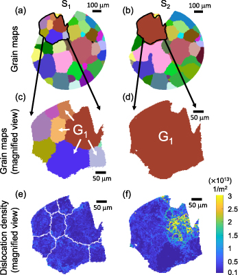
Figure 2. Grain and dislocation density maps for a selected cross-sectional slice of the cylindrical sample, measured at state  (left column) and
  (right column). (a), (b) Grain maps at state
  and
and  , respectively. An apparently confined region is indicated by a black contour. Each grain is indicated by a unique, random color. The same color is assigned to the same grain appearing in both states. (c), (d) Magnified view of the grain map for the confined region at state
  and
and  , respectively. Grain
  consumes the surrounding grains from state
  to
to  , respectively. (e), (f) Dislocation density field within the confined region at state
  and
and  , respectively.
Download figure:
Standard image High-resolution imageTo examine the effect of CHT on the microstructure evolution, it is necessary to track the change of the GSD over time, which requires a sufficiently large number of grains for meaningful statistics throughout the simulation. Since state  contains a large number of grains and corresponds to the starting point of the heat treatment cycle in the experiment, we use the GSD in state
  (evaluated from the entire volume; see figure 3(a)) to initialize a microstructure for the large-scale simulations. Likewise, the GSDs for states
  and
and  are shown in figures 3(b) and (c), respectively. Given the fact that the average grain radius for the entire three-dimensional (3D) volume increases by ∼40% from state
  to
to  in the experiment, we set this percentage of increase in the average grain radius as the stopping criteria in our simulation of one heat treatment cycle.
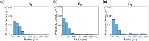
Figure 3. Grain size distribution for the entire volume of (a) state  , (b) state
  , and (c) state
  determined from the HEDM data. The grain size is evaluated as the equivalent radius, assuming a circular shape of the grain.
Download figure:
Standard image High-resolution image3. Methods
3.1. Individual dislocation density field
To account for the variation in intra-granular dislocation densities observed in the HEDM experiments, we introduce an individual dislocation density field,  , for each grain
  , which stores not only the initial dislocation density value for that grain but also what the dislocation density value would be if the grain boundary of the grain were to reach that position. While the exact mechanism by which the reduction in the dislocation density occurs has yet to be investigated, there are multiple mechanisms that would lead to an elimination of dislocations as a grain boundary migrates, including annihilation of dislocation pairs and absorption of dislocations onto grain boundaries [42, 43]. The enhancement of the rate by which these processes occur (vs. recovery in the bulk, which appears to be slow on the time scale of the experiment) is expected from the fact that grain boundary migration requires atomic rearrangements and consequently changes the strain fields. Below, we derive a model for dislocation density evolution that accounts for such a process, which is used to define
  .
.
Mathematically, it is reasonable to assume that the dislocation density is reduced at a rate,  , that is proportional to how many dislocations per unit volume exist at the grain boundary position as the grain boundary migrates:

where  is the distance traversed by the grain boundary and the inverse of
  provides the rate constant for the decay. This differential equation can be solved analytically, yielding

where  is the dislocation density just behind the initial grain boundary and the constant
  can now be identified as the length scale at which the dislocation density decays by a factor of
  in the wake of the migrating grain boundary. We assume that grain boundaries migrate in their normal direction, which is a simplifying assumption, and therefore the value of
  can be determined from a signed distance function using the level-set method (detailed in section S1 of the supplementary material).
We now describe how this model is implemented. As in figure 2, we denote the grain with index  as
as  . For each grain
  , we employ a time- and position-dependent order parameter field
  to track its evolution. The value of
  is 1 within the grain, 0 outside the grain, and varies smoothly from 1 to 0 across its interface. In this work, we omit the effect of recovery, and therefore the dislocation density at a certain position,
  , retains its initial value until the grain boundary from another grain reaches this point, at which time a reduced dislocation density is assigned, according to equation (2). Since we do not allow dislocation density to evolve otherwise, this model introduces discontinuities in the gradient of dislocation density, which persist; if we consider recovery, the magnitude of such discontinuities would gradually reduce and eventually vanish. We precompute the reduced dislocation density for each grain in regions not initially occupied by the grain and store these values into its individual dislocation density field
  , along with its initial dislocation density values within the grain. Specifically,
  is defined as

Here,  is the initial dislocation density within grain
  ,
,  is the dislocation density just behind
  's initial boundary, and
  is the signed distance between the point
  and the nearest point to the
  's initial boundary; note that the sign of
  is taken to be positive within the grain and negative outside, and therefore
  in equation (3). The term
  in equation (3) denotes a baseline dislocation density, i.e., the lower bound for the dislocation density measured in the experiment, that remains even after a long period of annealing. In general,
  is a spatially varying quantity, but we here assume it to be a constant for each grain, as discussed in section 3.4.2. We found that simulations with
  = 20
= 20  yield results that closely resemble the experimental observations, and thus we employ this value throughout this work. We estimate the baseline dislocation density
  to be
to be  m−2 by taking the average of the dislocation densities at state S2 for the regions outside grain
  's initial position (indicated in figure 2(c)). While this may slightly overestimate the base value because it may include some enhanced dislocation density near the initial grain boundaries, we deemed this assumption to be reasonable given the statistical variation and uncertainties in the measurements [44]. In addition, the determined value of
  is of the same order of magnitude as dislocation densities in well-annealed metals (
 m−2 to
  m−2 [45]), which supports the validity of the assumption. Further details are provided in section 3.4.2.
It is necessary to note that the values of  outside the boundaries of the initial grains should not be considered as physical values, other than the fact that it sets the value of the dislocation density if the grain boundary of
  sweeps past the point. Rather, at any point in time, the actual dislocation density is given by constructing it from
  , along with the set of order parameters
  , using the following interpolation function:

This formula is identical to those used in [16, 25, 37, 46], except that in these previous works,  was a constant associated with the
  grain, and therefore these models could not treat intra-granular inhomogeneity nor a decay in the dislocation density as the grain boundaries migrate.
To facilitate our understanding of dislocation density evolution based on the above formulation, we provide schematics in figure 4 showing the change in the dislocation density field as grain  consumes its surrounding grains. The grains that are adjacent to
  are omitted in figure 4(a) for clarity. Grain
  , indicated in blue, initially possesses dislocation density
  at the position of its grain boundaries. As it progressively consumes its surrounding grains with higher dislocation density (denoted by
  in figure 4) and reaches the point
  at time
  , the dislocation density reduces to a value given by
  . As the grain continues to grow to point
  at time
  , where by
  , the dislocation density value behind the migrating grain boundary reduces to the baseline dislocation density
  , which is the lower bound of the dislocation density. Beyond this point, the dislocation density behind the grain boundary remains at
  ; for example, when the grain boundary reaches point
  at time
  , the dislocation density at point
  reduces to
  .
.
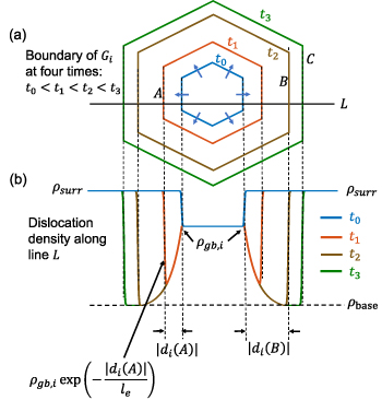
Figure 4. Schematics showing the evolution of a dislocation density field at four time-points when grain  consumes its surrounding grains, assuming an exponential decay of dislocation densities. For illustrative purposes, the first cycle is assumed. (a) Grain boundaries of
  at four times,
  , which are indicated in blue, red, brown, and green, respectively. The grains that are adjacent to
  are omitted for clarity. (b) The dislocation density field along the line
  in (a) at the four times. The baseline dislocation density, dislocation density at the grain boundary, and dislocation density of the surrounding grains are denoted by
  ,
,  , and
, and  , respectively. Note that the signed distance
  outside of the region initially occupied by the grain.
Download figure:
Standard image High-resolution image3.2. PF equations
A total free energy functional that encodes the thermodynamics of the polycrystalline material is given by the volume integral of the sum of three energy density terms:

We utilize the functional form proposed by Moelans et al [47] to calculate the bulk energy density,  :
:
where  is the bulk energy density coefficient, and
  is set to ensure a symmetrical order parameter profile across an interface, as discussed in [47]. The gradient energy density [20, 48],
  , is employed to penalize a sharp interface,

where  is the gradient energy coefficient. The values of
  and
and  are determined based on the grain boundary energy,
  , a material parameter, and the grain boundary width,
  , a model parameter, using the formula derived by Moelans et al [47]:


The grain boundary energy for Cu–Zn [49],  J m−2, is employed here for Cu–Al–Mn, due to a lack of data on the latter system. An approximate form [17], which neglects the energy of the dislocation core and assumes isotropic elasticity, is utilized to describe the stored energy density,
  , due to the presence of the dislocation density,
  , as
, as

where  GPa is the shear modulus for the
  phase of Cu–Al–Mn alloy at 650
  C, calculated by [14] based on [50]. The magnitude of the Burger's vector for the FCC copper [51],
  nm, is used here as an estimate value for the copper-rich Cu–Al–Mn alloy. The evolution of the order parameter
  is obtained via steepest descent, using Allen–Cahn dynamics [52]:

where  is the mobility parameter. Substituting equations (5)–(7) and (10) into equation (11) yields
3.3. Nondimensionalization of PF equations
We chose 40  as the length scale, which is on the order of the radius of a typical grain in our simulations. We divide all the lengths by
  to obtain their dimensionless forms. We select the bulk energy density coefficient
  in equation (6) as the energy scale and divide all the energies by
  to nondimensionalize them. We denote
  as the spatial average of
  over the entire computational domain (excluding the non-solid region defined by the dummy order parameter in section 4.1) and utilize this value to scale
  and
and  . After these scaling quantities are chosen, we set the time scale to

We divide the time by this scale, and rearrange the resulting equation, which results in the dimensionless form of equation (12). The dimensional and dimensionless quantities are summarized in table 1. The dimensionless quantities are denoted by their counterpart accompanied by an asterisk ( ) in their superscripts. We employ the dimensionless quantities for the study, which can be converted into dimensional quantities based on the scaling factors.
Table 1. Dimensional and dimensionless phase-field variables.
| Variable | Nondimensionalized variable |
|---|---|

|

|

|
|

|

|

|

|

|

|

|

|

|

|
3.4. Methods for setting up initial conditions
The initial condition for each simulation is composed of two parts: an initial microstructure described by a set of order parameters  , and a set of corresponding individual dislocation densities,
  . In this work, we perform two sets of 2D simulations. The first set of simulations directly imports a grain map from the experimental cross-sectional data containing a relatively small number of grains, while the second set of simulations leverages the GSD from the experimental data to initialize a synthetic microstructure that contains a large number of grains.
3.4.1. Initialization of order parameters.
First, the microstructure at state  captured in the experiment is processed to produce a set of binary fields
  . For the first set of simulations, the 2D grain map,
  , of the confined region at
  , which marks the region of each grain with a unique but consecutive integer, is used to initialize a set of
  fields according to

For the second set of simulations, the GSD calculated from the entire 3D volume of the sample at the  state (figure 3(a)) is converted to a 2D GSD by implementing an established method in stereology [53, 54] in a reversed manner, as detailed in section S2 of the supplementary material. The 2D GSD is then used to inform the selection of the locations of
  seeds of grains, as detailed in section S3 of the supplementary material. A set of binary fields
  is then constructed from the locations of
  seeds of grains, using the method discussed in section 3.5.
For both cases, the set of binary fields  is evolved via Allen–Cahn dynamics without the stored-energy for a dimensionless time of
  , just long enough to obtain the order parameters with diffuse interfaces,
  . The parameters employed for this smoothing process for the small- and large-scale simulations are summarized in tables 2 and 3, respectively. As mentioned earlier, the grain boundary energy for Cu–Zn [49],
  J m−2, is employed here for Cu–Al–Mn, which was consistent with Kusama's study [14]. For interfacial width, domain size, and grid spacing, both dimensionless and dimensional values are presented. Since bulk energy coefficient and gradient energy coefficient are model parameters that are calculated from the dimensionless values of grain boundary energy and grain boundary width, only dimensionless values of them are presented. The conversion of dimensionless time to dimensional time is complicated because it requires the mobility parameter
  , which depends on the temperature and was not reported for Cu–Al–Mn alloy under a non-isothermal annealing condition. Thus, this study focuses on qualitative agreement between the dynamics observed in simulations and experiments. Note that the initial microstructure for the small-scale simulations is derived from the experimental measurement and contained tiny grains that cannot be resolved by the PF model. Therefore, it was necessary to apply the smoothing operation longer (about twice as long) until these grains are eliminated during the smoothing process. In addition, slight adjustments were needed in the grid spacing and related parameters due to the domain size change.
Table 2. Parameters employed for the small-scale simulations to generate the order parameters from the binary fields. Dimensional values in parentheses denote numerical parameters (not physical parameters).
| Parameters | Variable | Value (dimensionless) | Value (dimensional) |
|---|---|---|---|
| Grain boundary energy |

| 1.67 
|
 J m−2 J m−2
|
| Grain boundary width |

| 0.1 | (4  m) m) |
| Domain size |

|

| 4.80  102 102
 m m |
| Grid spacing |

|

| (1  m) m) |
| Bulk energy coefficient |

|

| Not applicable |
| Gradient energy coefficient |

|

| Not applicable |
| Time step size |

|

| Not available |
| Duration |

| 100 | Not available |
Table 3. Parameters employed for the large-scale simulations to generate the order parameters from the binary fields. Dimensional values in parentheses denote numerical parameters (not physical parameters).
| Parameters | Variable | Value (dimensionless) | Value (dimensional) |
|---|---|---|---|
| Grain boundary energy |

| 1.46 
|
 J m−2 J m−2
|
| Grain boundary width |

|

| (3.5  m) m) |
| Domain size |

|

| 2.78  103 103
 m m |
| Grid spacing |

|

| (0.876  m) m) |
| Bulk energy coefficient |

|

| Not applicable |
| Gradient energy coefficient |

|

| Not applicable |
| Time step size |

|

| Not available |
| Duration |

| 50 | Not available |
3.4.2. Construction of individual dislocation density fields.
As seen in equation (3), the initial dislocation density  and the distance function
  for each grain
  are two required components to construct an individual dislocation density field
  . Although in reality a cycle of heat treatment involves continuous dislocation generation and microstructure evolution, we model this process by injecting all the generated dislocations,
  , at the start of the thermal treatment cycle; thus, this term is added to the baseline value before the microstructure evolution is simulated. A more sophisticated approach that considers the dynamic generation of dislocations during precipitation will be left for future work. Given the experimental observations that a majority of the second-phase particles is found on or near the grain boundaries and the fact that a small grain has a higher line length per unit area in two dimensions (equivalent to surface area per unit volume in three dimensions) than a large grain, we propose that the density of second-phase particles is higher in a small grain. Additionally, it is reported in [16] that the relationship between the grain-averaged dislocation density and the density of second-phase particles can be roughly described by a positive linear correlation. We therefore postulate that the value of
  is inversely proportional to the equivalent radius (assuming a circular shape),
  , of grain
  , according to

The value of  is estimated by substituting the known values of
  and
and  for grain
  within the confined region (see figure 2) into equation (15). To do so,
  is estimated by subtracting the baseline dislocation density from the average dislocation density of
  at
at  within its initial position at
  . The value of the equivalent radius
  is determined for
  based on its area at
  . Accordingly, the value of
  is found to be
  m−1.
m−1.
When considering multiple cycles, each cycle must be initialized based on either the initial state of the sample or the state from the previous cycle. Hereafter in this section, we add the cycle number on the superscript of the dislocation density to indicate the cycle number. The individual dislocation density at positions initially within grain  for the first cycle,
  , is set by adding
  to the baseline dislocation density
  :
:

To set the individual dislocation density at positions initially outside of grain  we first apply the level-set method discussed in section S1 of the supplementary material to obtain the distance function,
  , based on the order parameter
  . Since
  is a constant for the first cycle, as indicated by equation (16) and illustrated in figure 4(b) (see the blue line), the individual dislocation density at the grain boundary,
  , is equal to this constant value given by

Equation (3) is then employed to generate the individual dislocation density field  for the first cycle.
To reinject dislocations at the beginning of each subsequent cycle  , the value of the individual dislocation density at positions initially within
  for the subsequent cycle,
  , is set by adding
  to its individual dislocation density at the end of the previous cycle,
  :
:

We assume that after each cycle of grain growth, the value of dislocation density at the grain boundary of each remaining grain is reduced to a value that is sufficiently close to the baseline dislocation density. Thus, for simplicity, the individual dislocation density at the grain boundary for the cycle  (where
  ),
),  , is set again using equation (17). Then, equation (3) is employed to generate the initial dislocation density field
  , where
  .
.
3.5. Assigning multiple grains to an order parameter
Although the implementation is simple when an order parameter is used to track one grain, the computation becomes expensive when the simulation involves a large number of grains, as in the second set of simulations. To enable large-scale simulation of microstructure evolution in an efficient manner, we require the capability to track multiple grains with one order parameter, which reduces the total number of order parameters required for the simulations. However, it is necessary to ensure that the grains tracked by the same order parameter do not overlap during the microstructure evolution to avoid grain coalescence (and, for our model, that the decaying individual dislocation density fields do not overlap, which would introduce numerical artifacts). The grain remapping schemes [32, 55, 56] have been proposed in the literature for PF simulations of grain growth, which reassign a grain to a different order parameter when the grain is too close to another grain tracked by the same order parameter. However, the standard remapping scheme cannot be applied without modifications because of the necessity to track the decay in the dislocation density outside of the grains. Therefore, we take a simpler approach in which grains are placed sufficiently far apart initially and are not dynamically remapped. In practice, we assign up to nine grains to one order parameter to reduce the number of required order parameters (and thus the number of equations to be evolved) and employ a corresponding individual dislocation density field to track the decay in dislocation densities for these grains. The detailed procedure is described in section S4 of the supplementary material.
4. Results and discussion
4.1. Microstructure evolution within a confined region
In this section, we apply the PF model to study the evolution of microstructure and dislocation density within a confined region observed in the experiment (see figures 2(c)–(f)), as discussed in section 2. We select  as the interfacial width, which is ∼1/10 of the radius of a typical grain in our simulations and is sufficient to resolve the grains in the confined region. The order parameters are initialized using the method discussed in section 3.4.1. Since the boundary of the confined region is not rectangular, we utilize a dummy order parameter, which is not evolved throughout the microstructure evolution, to describe the area surrounding the confined region. The individual dislocation densities are initialized using equation (3), with
  given by equation (16) and
  given by equation (17). The dimensionless parameters employed for the simulation are summarized in table 4.
Table 4. Parameters employed in the simulation for microstructure evolution of the confined region. Dimensional values in parentheses denote numerical parameters (not physical parameters).
| Parameters | Variable | Value (dimensionless) | Value (dimensional) |
|---|---|---|---|
| Grain boundary energy |

| 1.67 
|
 J m−2 J m−2
|
| Grain boundary width |

| 0.1 | (4  m) m) |
| Domain size |

|

| 4.80  102 102
 m m |
| Grid spacing |

|

| (1  m) m) |
| Bulk energy coefficient |

|

| Not applicable |
| Gradient energy coefficient |

|

| Not applicable |
| Time step |

|

| Not available |
The initial microstructure is shown in figure 5(a). Each grain is assigned to a unique number from 1 to 8. The color indicates the dislocation density within the grains. As shown in figure 5(b), grain 2 is rapidly consumed by the neighboring grains 3, 4, and 7. This behavior is expected since grain 2 possesses a higher dislocation density and a smaller size than the surrounding grains, leading to a large combined driving force due to capillarity and stored energy. As microstructure evolution proceeds, grains 3, 4, 5, and 6 are continuously consumed, as shown in figures 5(c) and (d). It is worth noting that the traversed regions that are far away from the initial boundary of the growing grains, such as the left regions of grains 1 and 8, have a nearly uniform deep blue color, implying the reduction of dislocation density to a baseline value. In addition, some of the grain boundaries, such as the one between grains 1 and 8 in figure 5(d), become curved during microstructure evolution. Such curved boundaries, often associated with island grains or peninsula grains, have been reported in samples that have undergone mechanical deformation and subsequent (isothermal) annealing leading to AGG [57, 58]. The simulation results thus indicate that such curved grains could also be induced by heat treatment alone without mechanical processing. Since grain 8 (with radius ∼92  m) is slightly larger than grain 1 (with radius ∼90
  m), the assigned initial dislocation density for grain 8 (∼1.17 × 10¹³ m−2) is lower than that for grain 1 (∼1.19 × 10¹³ m−2). Consequently, grain 8 eventually consumes grain 1, as shown in figures 5(e) and (f), which does not agree with the experimental observation that grain 1 consumes grain 8, as shown in figures 2(c) and (d).
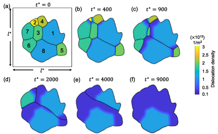
Figure 5. The evolution of microstructure and dislocation density within a confined region found in the experiment (see figure 2). A unique number from 1 to 8 is assigned to each grain. Dislocation densities of all the grains are initialized with equation (16). The color indicates the dislocation density. A black box is plotted in (a) to indicate the simulation domain.
Download figure:
Standard image High-resolution imageThe disagreement could arise from a few potential reasons. First, the simulation is confined to 2D, and the evolution of a cross section within a 3D volume may differ from that of a 2D simulation. Moreover, although the density of the second-phase particles is in general expected to be larger within a smaller grain, there may be statistical variations due to the stochastic nature of precipitate nucleation, growth, and subsequent dissolution that produce dislocations. Finally, it has been known that grain boundary energies are anisotropic, depending on not only the crystalline orientations of the pair of grains but also the relative orientation of the grain boundary plane [59]. The resulting variation in grain boundary energies would result in different probabilities of precipitating second-phase particles on or near grain boundaries, leading to a spread in the density of dislocations produced by the precipitates. Therefore, in reality, the dislocation density within a grain will likely not follow equation (15) exactly, and it is plausible that grain 1 has a lower dislocation density than grain 8. By conducting a parametric sweep, we determined that when the dislocation density of grain 1 is reduced by ∼16% to 1013 m−2, grain 1 consumes grain 8 during the simulated evolution. The results of this simulation are shown in figure 6. The early evolution of the two simulations are very similar, as can be seen by comparing figures 5(a)–(c) and 6(a)–(c). On the other hand, during the later stage, grain 1 progressively consumes grain 8, as shown in figures 6(d) and (e), and it is the only grain that remains at the end of the simulation, as shown in figure 6(f). The high dislocation density at grain 1's initial position and the low dislocation density in the surrounding region closely resemble the experimental observations from figure 2(f). Although a quantitative agreement is not expected because of the 2D nature of the simulations and is therefore not a goal of this work, the observed similarities provide support for the proposed model.

Figure 6. The evolution of microstructure and dislocation density within a confined region found in the experiment (see figure 2). As in figure 5, a unique number from 1 to 8 is assigned to each grain. Dislocation densities of grains 2 through 8 are initialized with equation (16). The dislocation density of grain 1 is reduced by ∼16% from the value given by equation (16), which resulted in a better match with the experimental observation. The color indicates the dislocation density. A black box is plotted in (a) to indicate the simulation domain.
Download figure:
Standard image High-resolution image4.2. Large-scale simulations
In this section, we perform a set of large-scale simulations to examine the effect of CHT on the microstructure evolution. To maintain computational feasibility, the smallest resolvable grain in the simulations is chosen to have a radius of  . This grain radius requires the interfacial width (defined by order parameter values from ∼0.1 to ∼0.9) to be no larger than 3.5
  such that the bulk region within the smallest grain occupies at least 50% of the area, assuming a circular shape of the grain. We initialize the order parameters using the method discussed in sections 3.4.1 and 3.5. The individual dislocation densities are initialized using equation (3). For this equation, the values of
  are given by equation (16) when the dislocations are injected for the first time and by equation (18) when the dislocations are injected for the second and the third times. The values of
  are given by equation (17). The dimensionless parameters employed for the simulations are summarized in table 5. Periodic boundary conditions are utilized throughout the simulations.
Table 5. Parameters employed in the large-scale simulations. Dimensional values in parentheses denote numerical parameters (not physical parameters).
| Parameters | Variable | Value (dimensionless) | Value (dimensional) |
|---|---|---|---|
| Grain boundary energy |

| 1.46 
|
 J m−2 J m−2
|
| Grain boundary width |

|

| (3.5  m) m) |
| Domain size |

|

| 2.78  103 103
 m m |
| Grid spacing |

|

| (0.876  m) m) |
| Bulk energy coefficient |

|

| Not applicable |
| Gradient energy coefficient |

|

| Not applicable |
| Time step (with stored energy) |

|

| Not available |
| Time step (without stored energy) |

|

| Not available |
The initial microstructure, which contains 1778 grains, is shown in figure 7(a). It can be observed from the figure that a number of small grains are clustered in a chain-like structure. This arrangement is reasonable in 2D given the facts that a large portion of small grains was observed in the experiment at state  (see figure 3(a)) and that these small grains would have to cluster in order to avoid an unphysical (non-equiaxed) grain morphology. The high dislocation density of these small grains yields a high stored energy as compared to their surrounding grains, and consequently, these grains are rapidly consumed, as shown in figure 7(b). The microstructure at the end of the first cycle is shown in figure 7(c). Most grains with high dislocation densities (i.e. yellow grains) are consumed by their surrounding grains at this stage and the large grains next to these small grains become larger. The corresponding GSDs are shown in figure 8. Note that the probability is scaled to yield an area of unity under the curve. It can be seen that GSD broadens during this cycle (figures 8(a) and (b)), primarily due to the increase in the average grain size. A second cycle is then simulated, which consists of reinjections of dislocations to the microstructure and subsequent microstructure evolution. The increase of dislocation densities is inversely proportional to the grain radius (equation (15)), and therefore the smaller grains experience a higher increase in dislocation densities, as shown in figure 7(d). Microstructures at an intermediate stage and at the end of the second cycle are shown in figures 7(e) and (f), respectively. The GSD continues to broaden, as shown in figure 8(c). A second peak in the GSD appears after the third cycle, as shown in figure 8(d). The comparison of scaled GSDs for each cycle is provided in figure S4(a) of the supplementary material, in which all the radii are divided by the average radius. The scaled GSD for the simulation with stored energy is clearly not self-similar. Instead, it continues to evolve throughout the three simulation cycles, exhibiting a slight broadening especially at the later cycles, and a bimodal distribution may start to develop at the end of the third cycle. It has been suggested that a bimodal GSD is one of the signatures of AGG [2, 3].
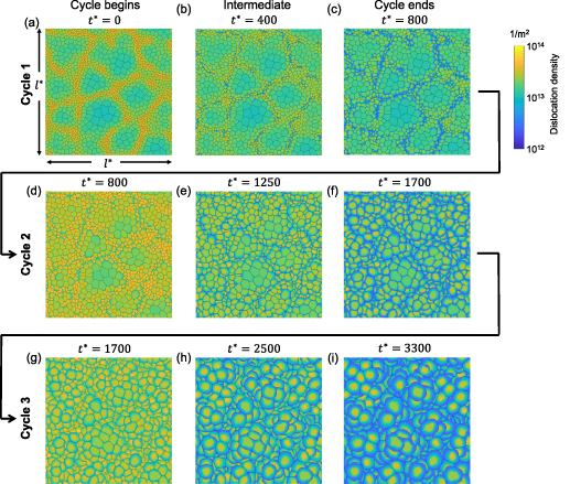
Figure 7. Stored-energy-driven microstructure evolution, after dislocations were injected (a)–(c) once, (d)–(f) twice, and (g)–(i) three times. Each cycle ends when the average grain radius increases by 40%. The dimensionless time  is labeled. The color indicates the dislocation density.
Download figure:
Standard image High-resolution image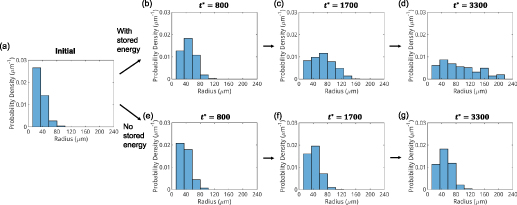
Figure 8. Grain size distributions (GSDs) during the microstructure evolution: (a) at the initial time; (b)–(d) after first, second, and third cycles with stored energy, where  ,
,  , and
, and  , respectively, note the cumulative time; and (e)–(g) at
  ,
,  , and
, and  for a simulation without stored energy. The probability is scaled to yield an area of unity under the curve.
Download figure:
Standard image High-resolution imageWe note that the GSD calculated from the simulated data (figure 8(b)) do not match the experimental result in the  state (see figure 3) on the extreme ends of the distribution. Besides the difference in the dimensionality between the simulation and experiment, there are additional reasons for the discrepancies. On the low end of the radii, the simulation misses some of the smallest grains due to the diffuse interface effect, while the experiment may overestimate the number of small grains due to the noise in the data. On the high end of the radii, the experiment had temperature gradient over the sample, which led to faster grain growth in the hotter end, where the large grains were identified. Furthermore, the timing of the end of the cycle is approximated by the increase in the radius, which introduces additional uncertainty.
To confirm that dislocation injections are necessary to yield persistent AGG [60], a simulation that omits the driving force due to the stored energy difference is performed. To allow for a direct comparison, an identical initial microstructure is employed, as depicted in figure 9(a). The microstructure at times  ,
,  , and
, and  during the evolution is shown in figures 9(b)–(d), respectively, which correspond to the final net times of the three cycles for the stored-energy-driven grain growth (see figures 7(c), (f), and (i)). In this case, the large grains still progressively consume the smaller grains surrounding them, due to capillarity. To quantify and compare the rate of the microstructure evolution between the simulations with and without the stored energy, we show the average grain radius as a function of time for the two cases in figure 10. The average grain radius during the microstructure evolution with stored energy for cycles 1, 2, and 3 are indicated by red, blue, and black dots, respectively. The average grain radius during the microstructure evolution without stored energy is indicated by green dots. A much faster increase in the average radius is observed when stored energy is considered, which indicates that the microstructure evolution proceeds more rapidly when dislocations are injected via CHT. Additionally, at the start of each cycle, there is a rapid increase in the average radius, which is due to the large variation in initial dislocation densities. Then, the growth rate decreases as the stored-energy driving force reduces and the system shifts toward NGG. An additional abrupt increase in the average radius in the middle of cycle 3, observed from time
  to
to  , is caused by a significant fraction of grains (14 out of 246 grains) that disappeared between these two times. Unlike the apparent broadening of the GSD observed in the evolution of microstructure with dislocations, the GSD for capillary-driven grain growth only slightly broadens (see figures 8(e)–(g)). In addition, none of the grains are observed to grow abnormally faster than the others. Consequently, the GSD remains singly peaked from
  to
to  . The convergence to self-similarity is observed in the scaled GSD, as shown in figure S4(b) of the supplementary material.
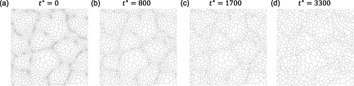
Figure 9. Capillary-driven microstructure evolution, using the same initial microstructure as in figure 7(a). Four snapshots are shown at times (a)  , (b)
, (b)  , (c)
, (c)  , and (d)
  .
.
Download figure:
Standard image High-resolution image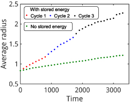
Figure 10. Dimensionless average grain radius vs. dimensionless time. The red, blue, and black dots indicate the average grain radius during microstructure evolution with the stored energy contribution for cycles 1, 2, and 3, respectively. The green dots indicate the average grain radius during microstructure evolution without the stored energy contribution.
Download figure:
Standard image High-resolution image
To further examine the necessity of recurrent dislocation injections to continuously provide stored-energy driving force, we performed an additional simulation in which the dislocations are only injected once at the beginning. The average grain radius as a function of time from this simulation is shown in figure S3 of the supplementary material, in which red crosses indicate the continued portion, along those of the three-cycle simulation. The microstructure evolution with one-time dislocation injection gradually turns slower, and eventually the rate reduces to a value that is close to that of capillary-driven grain growth, suggesting a progressive transition from stored-energy-driven grain growth to capillary-driven grain growth. In order to prevent such transition, dislocation reinjections are necessary, which provide continuous stored-energy driving force to maintain the rate of microstructure evolution.
5. Conclusions
We developed a PF model for the evolution of microstructure with a spatially varying dislocation density and a reduction in the dislocation density as a grain boundary migrates. We conducted simulations based on the assumption that the smaller grains having higher grain boundary length per unit area (equivalent to surface area per unit volume in 3D) have a higher density of second-phase particles and thus a higher density of dislocations injected. The simulation predicted a microstructure that closely resembles the experimentally observed microstructure within a region that was confined within a nearly static boundary in the experimental dataset. In addition, the model was utilized to simulate three cycles of stored-energy-driven grain growth within a large microstructure, during which non-self-similar evolution was observed. In contrast, a simulation without the effect of stored energy yielded a near self-similar evolution. In particular, when the stored energy was included assuming that density of dislocations that is injected scales as the inverse of the grain radius (which is expected if the source of dislocations is due to precipitation and dissolution of second-phase particles on or near grain boundaries), it was found not only that grains grew much faster but also the larger grains preferentially grew. Moreover, although the rate of grain growth with stored energy is much faster at the beginning of each cycle as compared to that without stored energy, the former decreases at the later stage of each cycle as the stored-energy driving force reduces with time and the system shifts toward NGG. Therefore, CHT (multiple repetitions of thermal cycling) is necessary to provide an inexhaustible stored-energy driving force.
These simulation results offer a possible mechanism behind persistent AGG during CHT. Additionally, we provided an integrated experimental-computational workflow, which utilizes the information from experiments to inform grain-growth models and its parameterization. While we here limited our efforts to 2D simulations as a proof-of-concept, the workflow can be easily adapted to perform more time-consuming, but more accurate, 3D simulations, as well as to include additional physical considerations, such as recovery. Therefore, our work provides a foundation for future development of simulation tools capable of quantitative predictions of microstructure evolution during non-isothermal heat treatment, which will ultimately facilitate the design of optimized processes for solid-state manufacturing.
Acknowledgments
This work was supported by the United States National Science Foundation under Award No. DMR-2104786. The computational resources for model development and validation were provided by (1) the National Energy Research Scientific Computing Center, a US Department of Energy Office of Science User Facility located at Lawrence Berkeley National Laboratory, operated under Contract No. DE-AC02-05CH11231 and (2) Stampede2 at the TACC through allocation No. TG-DMR110007 from the Extreme Science and Engineering Discovery Environment, which was supported by National Science Foundation Grant Number #1548562. The computational resource for the large-scale simulations reported in this work was provided by Anvil at the RCAC through allocation No. TG-DMR110007 from the Advanced Cyberinfrastructure Coordination Ecosystem: Services & Support (ACCESS) program, which is supported by National Science Foundation Grants #2138259, #2138286, #2138307, #2137603, and #2138296. The authors would like to thank David Montiel for the useful discussion. The data presented in this work [61] is published at Materials Commons (materialscommons.org) [62].
Data availability statement
The data that support the findings of this study are openly available at the following URL/DOI: https://doi.org/10.13011/m3-x0qx-yf02.
Code availability
All codes from this study are available from the corresponding author upon reasonable request.
CRediT authorship contribution statement
Guanglong Huang: conceptualization, methodology, formal analysis, investigation, writing—original draft, writing—review & editing, visualization. Alexander Mensah: methodology, investigation, software, writing—review & editing. Marcel Chlupsa: conceptualization, investigation, methodology, formal analysis, writing—original draft, writing—review & editing. Zachary Croft: validation, investigation, formal analysis, writing—original draft, writing—review & editing. Liang Qi: methodology, writing—review & editing. Ashwin J. Shahani: conceptualization, funding acquisition, investigation, project administration, supervision, writing—review & editing. Katsuyo Thornton: conceptualization, funding acquisition, investigation, methodology, project administration, resources, supervision, validation, writing—review & editing.
Conflict of interests
The authors declare that they have no known competing financial interests or personal relationships that could have appeared to influence the work reported in this paper.
Supplementary material (0.7 MB PDF) Supplementary material for the main text