

Abstract
Thermally induced phase transformation in NiTi shape memory alloys (SMAs) shows strong size and shape, collectively termed length scale effects, at the nano to micrometer scales, and that has important implications for the design and use of devices and structures at such scales. This paper, based on a recently developed multiscale model that utilizes molecular dynamics (MDs) simulations at small scales and MD-verified phase field (PhF) simulations at larger scales, reports results on specific length scale effects, i.e. length scale effects in martensite phase fraction (MPF) evolution, transformation temperatures (martensite and austenite start and finish) and in the thermally cyclic transformation between austenitic and martensitic phase. The multiscale study identifies saturation points for length scale effects and studies, for the first time, the length scale effect on the kinetics (i.e. developed internal strains) in the B19' phase during phase transformation. The major part of the work addresses small scale single crystals in specific orientations. However, the multiscale method is used in a unique and novel way to indirectly study length scale and grain size effects on evolution kinetics in polycrystalline NiTi, and to compare the simulation results to experiments. The interplay of the grain size and the length scale effect on the thermally induced MPF evolution is also shown in this present study. Finally, the multiscale coupling results are employed to improve phenomenological material models for NiTi SMA.
Export citation and abstract BibTeX RIS
1. Introduction
Experimental and/or computational study of the martensitic phase transformation (MPT) in SMAs such as NiTi is demanding, mainly because of the complexity and stochasticity in the formation of different martensite variants [1–8]. Free surfaces interfere with the formation of variants, leading, especially at small scales where the ratio of free surface area to volume is large, to significant size and scale effects, collectively termed as length scale effects [9–15]. Not only the length scales affect the phase fraction evolution and the thermally cyclic hysteresis, but also affect the transformation temperatures (martensite and austenite start and finish) and the overall constitutive response of the material. Size effects have been studied recently [8, 11–15], but shape effects have not, even though a lot would be learned from such studies that would aid the design and development of nanoscale SMA-based devices such as sensors and actuators. Computational studies employing classical molecular dynamic (MD) simulations at the atomic level [11, 13–15] or stochastic phase field (PhF) simulation methods at the mesoscale level [8, 16] demonstrate size effects (due to the presence of free surfaces) on the phase transformation process of NiTi SMA. Findings (experimental or computational) include: (a) equiatomic NiTi thin samples [9, 10, 17] and nanoparticles [11, 13] showing nucleation and growth of unexpected stable crystal structures at the nanometer scale; (b) multiple transformation paths from B2 to B19' variants [13, 18, 19] in nanograins NiTi; and (c) highly stable square nanowires against torsional buckling, as compared to circular ones [20].
During thermally induced MPT internal strains develop in both B2 (austenite) and B19' (martensite) phases. Recent experimental studies by Ahadi and Sun [21–23] demonstrate the effect on grain size on the stress-induced martensitic phase transition process, in polycrystalline superelastic NiTi SMA, at the nanoscale. It is concluded that, with the reduction in grain size (less than ∼60–68 nm), the stress hysteresis loop size and temperature dependence of phase transformation stress reduce drastically, leading to the vanishing of the stress hysteresis and to the collapse of the Clausius–Clapeyron equation [21]. Also, measurement of lattice parameters and associated lattice strains shows that with reduction of grain size, the phase transformation mechanism changes into a continuous lattice deformation (inside the nano grains), as compared to the conventional nucleation and growth mode in coarse-grained polycrystals [23]. In another study by Ahadi and Sun [22] it is observed that for polycrystalline NiTi SMA, the effect of strain rate on the hysteresis loop area and transformation stress reduces with the reducing grain size and vanishes for any grain size below approximately 10 nm. Therefore, it becomes very important to have an appropriate understanding of the nature and evolution kinetics of such internal strains, because (a) they govern the stability of different phases and (b) they can be used in constitutive modeling of the SMA as an internal variable in conjunction with the B19' variants and B2 phase fraction. These strains have been computationally studied for the B2 phase [24], but not explicitly for the B19' phase. This is mainly because the developed internal strain in the martensite variants varies with the variants. Based on crystallographic theory [25–27], it is possible to obtain the internal strain tensor of individual B19' variants, thus, based on the phase fraction of different B19' variants, these strain tensors can be used to obtain the total internal strain in the spatial domain of B19'. However, evolution of different phases and internal strains are intercoupled, thus, to study the entire phase transformation process (B2 ↔ different B19' variants) requires a large number of nonlinear simulations which is computationally challenging, at least for the atomic and mesoscale scales. The complexity increases for polycrystalline NiTi due to the presence of grain boundaries. Despite of its importance, the interplay of cell/specimen size and grain size has received little attention at fine and meso scales, perhaps because of the difficulties in addressing it. Some attempts to shed light in such interplay are reported in [28, 29] albeit for mechanical properties.
Along the same lines, it has been observed that due to the evolution of different variants of B19' and B2 phases, the phase transformation process becomes inherently stochastic in nature [1, 3, 8] and occurs hierarchically over a very wide range of spatiotemporal scales [1, 3, 8, 15]. However, the ins and outs of such aspects remain poorly understood. It is worth studying and understanding such length-scale-dependent stochastic phase transformation and then linking the length scales to the propagation or transfer of stochasticity from micro and meso scales to macro/continuum scales. Such multiscale coupling would not only provide a robust material model at the continuum level, but would also enable the incorporation of the effects of length scales in the evolution kinetics of the phase transformation process. In this context, review papers [30, 31] and other field specific studies [32–34] provide details about computational modeling of relevant multiscale and multiphysics problems (MSMPs). Wavelet-based MSMP methods have received sufficient attention for addressing both spatial [8, 35–37] and temporal scaling [38–41]. Further, wavelet-based techniques provide advantages over other multiscale methods because of their ability to perform scale-wise data fusion, flexibility in upscaling and downscaling of the dynamic features, and finally, capability in preserving non-stationary features in the dynamics which is lost or significantly distorted by other types of infinite basis transforms (e.g., Fourier analysis). Therefore, herein, small size NiTi samples are studied via MD simulations, and larger size samples are studied via stochastic PhF simulations. A concurrent multiresolution (wavelet) based multiscale methodology, namely the compound wavelet method (CWM) [8, 35–40] is used to link the MD and PhF simulations along spatial scales, yielding a length-wise compound representation of the thermally induced MPT process. Finally, the CWM method is used to feed the information on length scale effects (obtained from the MD and PhF simulation of NiTi single crystals), onto a phenomenological material model, which was originally developed by Zotov et al [42] based on their experimental study.
It can be expected that, at the atomic to meso scales, interaction of the different phases (B2 and B19') with the free surfaces causes significant variation in the phase fraction evolution process and transformation kinetics, as briefly addressed in recent computational studies by the authors [8, 15]. However, in those previous studies by authors [8, 15], as well as in some other relevant studies [11, 13], the coupled effect of grain size and length scale, on the thermally induced MPT was not addressed. Rather, all those previous studies [8, 11, 13, 15] mainly explore the effects of the side length (thin samples of constant thickness i.e. 2 nm) or the size effect (nano particles or spheres) on the thermally induced MPT process for NiTi single crystal. A general spatial multiscale coupling framework is proposed by the authors [8], to transfer information from fine to coarse scales in the solid to solid phase transformation process. In that study [8], considering a single size case (i.e. for the simulation cell where the martensite phase fraction (MPF) saturates), uncertainties in the evolution (due to the temperature) of B2 (austenite) phase and different B19' variants (martensite) are propagated from small scales (micro/meso level) to coarse scales (continuum level). Thus, this study extensively broadens the results from the previous studies by the authors [8, 15] and in addition:
- Explicitly studies the effect of length scale (i.e. thickness and side length) on phase transformation process i.e. evolution kinetics and transformation temperatures of single crystal NiTi sample.
- For the first time, shows, computationally, the effect of length scales and temperature, on the development of internal strain in the B19' phase.
- Performs MSMP simulations to link different length scales and transfer the statistical information of length scale effects from micro (i.e. atomic) and meso (i.e. PhF) scales to the macro (continuum) scale.
- Develops a unique and novel multiscale method for indirect modeling of the phase transformation process in polycrystalline NiTi by employing the wavelet coefficients from single crystal simulations of various size cells.
- Employs PhF simulations to demonstrate the interplay of grain size and length scale effect on the thermally induced MPF evolution, for polycrystalline NiTi.
- Finally, using the MSMP coupling results, improves already existing, continuum scale, phenomenological constitutive models.
2. Simulation methods and multiscale coupling
The MD and PhF methods used in this study, as well as the CWM methodology for linking the results from the two simulation methods are described in detail in a very recent study by the authors [8]. Heat diffusion is modeled herein using the lattice Boltzmann method (LBM), similarly to what is used in [8]. Therefore, a brief description of those methods are provided herein. The key points that relate to the objective of the present paper are only addressed, and the paper concentrates on the results relevant to shape effects and internal strain in the B19' phase, the strains developed in B19' and on modeling polycrystalline samples.
2.1. MD potential, simulation process and structural characterization
MD simulations are performed employing the Finnis–Sinclair many body interatomic potential [4, 8, 11, 14, 15, 43], developed based on the embedded atom method (EAM) and considering a tight binding second moments approximation (TBSMA) theory. Quasi-static MD simulations are performed in LAMMPS [44], for temperature driven phase transformation process. Brief description of the simulation process is provided subsequently, while more details are available in recent studies by the authors [8, 15]. This EAM potential was initially proposed by Lai and Liu [43], based on the second-moment approximation of tight-binding theory (TBSMA). According to this potential, the total energy of the system over all atoms is expressed as
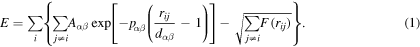
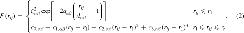
The first term in (1) indicates the pairwise interaction energy and the second term represents many-body effects. Recently the many-body interaction part (second term in (1)) of Lai and Liu potential has been modified by Zhong et al [4, 45], where the second term in (1) is expressed through
In (1) and (2),  and
and  denote atoms,
  denote the type of atoms (i.e. Ni or Ti), and
  and cut-off radius
  are adopted as 4.0 Å and 4.2 Å, respectively. Different parameters of this potential are determined through fitting the properties (i.e. lattice parameters, cohesive energy, elastic constants and vacancy formation energy) of the B2 phase at 0 K temperature, from first principles calculations [4]. More details about this EAM potential parameters are provided in Zhong et al [4].
To study length scale effects, free boundary conditions in all three directions of the simulation cell are imposed. In doing so, periodic boundary condition is used in all sides, with vacuums (empty space) all around the simulation cell are considered. In every direction, a minimum 20 Å empty space is provided, while the potential cutoff radius  is 4.2 Å. This eliminates the possibility of interaction between surface atoms, due to the periodic boundaries and thus enables the capturing of length scale effects. Based on such boundary conditions, at constant temperature, at first NPT simulation, followed by NVT equilibration is performed. The size and thickness of the examined cells are described in the results and discussion section. Initially, pristine B2 crystal structures, i.e. 3D simulation cells with the crystallographic orientation [110], [
 10] and [001] are considered. For the horizontal plane, directions along thickness [110] and along one side length [
 10] are considered. For the vertical direction, the [001] crystal orientation is considered. The simulation process is as follows. First, a pristine austenite sample is relaxed using an energy minimization method. Then the sample is subjected to a velocity distribution (at a constant temperature, controlled via proper thermostat and barostat) and held for 360 ps, under an NPT stabilization where the systems pressure is kept constant at 0 bars. The NPT stabilized sample is then subjected to NVT conditions for an additional 240 ps. The atomic coordinates were averaged over 20 ps in order to avoid effects from thermal fluctuations. In each case of NPT or NVT stabilization, the adopted time step is
  ps. During simulation, the temperature and pressure are controlled by a Nose–Hoover thermostat and Berendsen barostat. It has been verified that the simulated cells are well-equilibrated and the fluctuations in the total energy and temperature are smaller than the 0.001 eV/atom and 0.50 K, respectively. Finally, the well equilibrated NVT simulations (i.e. averaged over last 20 ps) is used to report the results.
To distinguish austenite B2 phase from the different martensite B19' phase variants, the bond length based order parameter proposed by Mutter and Nielaba [8, 11, 12, 15, 46] was adopted. This order parameter has a value of −1.0 and +1.0 for pristine B2 and B19' structures, respectively. It is expressed as

where bond length parameters are  The order parameter becomes +1.0 for the martensite B19' phase when
  and
and  For the austenite B2 phase
  and thus the value of the order parameter becomes −1.0. However, the lattice parameters of B2 and B19' phases change due to the linear thermal expansion or contraction
  and due to the internal strains
  that develop during the phase transformation process. Thus the order parameter shows a narrow Gaussian distribution around −1.0 and +1.0 for the B2 and B19' phases, respectively [8, 15, 24]. More details about this order parameters can be found in [8, 11, 12, 15, 24], and in the supplementary material.
2.2. PhF simulation: model and method
PhF simulations, a widely used and validated methodology [7, 16, 24], is employed to simulate the MPF evolution, based on the Ginzburg–Landau type polynomial energy function [7, 8]. In PhF simulations, austenite B2 transforms into 12 different variants of monoclinic martensite B19', with all field variables evolving stochastically over the simulation domain. The growth or evolution rate of the ith field variable  can be expressed through the time dependent Ginzburg–Landau (TDGL) kinetic equation as [7, 8]

where  is the kinetic coefficients matrix,
 and
and  represent the driving force acting on the jth field variable due to the local free energy density
  gradient energy density
  and elastic energy density
  respectively, and
  is the Langevin noise term to incorporate the stochasticity in the evolution of the B19'variants.
For  the driving force on the ith PhF variable is considered that it does not affect the evolution of jth PhF variable, thus
  where
where  is the Kronecker delta. Further, from the fluctuation–dissipation theorem [7], the correlation function of the Langevin noise term in the spatiotemporal domain can be expressed as a function of temperature
  where
where  is the Boltzmann constant,
  is simulation temperature and
  is the Dirac delta function. With this, (4) results into

Next, the energy density functions can be expressed as [7, 8]


In (6a),  represents the free energy density of the austenite phase,
  the difference in the free energy between austenite and martensite phase at temperature
  and
and  are constants that control the shape of the free energy function. In (5b), for isotropic gradient energy coefficient
  is assumed the same for all the field variables, i.e.
  and thus (6b) will can be rewritten as [7, 8]

In (6c),  is the linearized strain tensor, i.e.
 is the nonlinear stress-free strain due local phase transformation, i.e.
  and
and  is the 6 × 6 isotropic elasticity tensor in the Voigt notation system [7, 8]. Elastic interactions play a critical role in the evolution of MPF, thus, the accurate estimation of the elastic energy density is important. Since in the present study no external strain is applied (i.e.
  ), (6c) can be written as [7, 8]
where  represents the transformation strain tensor associated with the ith PhF variable [7, 8]. More details about the estimation of
  is provided in the supplementary material. Here,
  represents the stress-free strain (i.e. internal strain tensor in B19'), which arises due to local MPT from B2 to B19', expressed as

Therefore, the associated driving forces for the evolution of jth field variable can be described through the following set of equations


With all the terms in TDGL kinetic equation in (5) obtained, the stochastic spatiotemporal evolution of any field variable (e.g. the jth field variable) can be expressed as [7, 8]
Equation (11) is easily normalized in terms of length and time scale. By employing evenly spaced grid size  and time steps
  in (11), it follows that
where dimensionless time and time steps are expressed in terms of real time  and time steps
  i.e.
i.e.  and
and  and the dimensionless spatial coordinate system is expressed in terms of the grid size
  i.e.
i.e.  and
and  denotes the normalized isotropic gradient energy coefficient. Finally, the normalized Langevin noise term
  is generated as a random number from the spatiotemporally uncorrelated normal distribution with zero mean and variance of
For the simulation process, initially 2D B2 simulation cells of different sizes (from 32 nm to 2048 nm) are considered. The crystallographic orientation of the B2 simulation cells are adopted as [110] (along x direction) and [001] along (y direction) and then the simulation cells are stabilized at constant temperature, as detailed subsequently. The spatial and temporal resolutions are adopted as  and
and  respectively, and simulations are performed for a total time of
  out of which, for the first
  the simulation is perturbed by uncorrelated Langevin noise. Convergence of the simulation process is ensured by comparing different statistical measures of the MPF between two consecutive iteration steps, i.e. iteration is stopped once
  Here, for any variable
  the difference in value between two consecutive iteration steps is expressed as
  and the tolerance limit is adopted as
  Further details about the PhF simulation process is provided in [8].
2.3. LBM: heat transfer
Heat transfer in the simulation domain is modeled with the LBM that has received significant attention in simulation of transport processes [47–53]. Considering an isothermal process for heat transfer, Peng's implementation of thermal LBM [48] is a simplified form of He et al [47] thermal LBM. It considers that heat diffuses through the NiTi medium, and heat is dissipated during phase transformation. For the transient case, the heat diffusion equation with energy dissipation can be expressed as

where 

 and
and  are the density, thermal conductivity, heat capacity and heat energy dissipation, respectively.
Here, the LBM solves the generalized heat diffusion equation via propagation and collision steps, employing specific so-called elements [8, 51–53]. In the present study, the D2Q9 lattice configuration is used for the transport process [8, 51–53]. The temperature dependent thermal conductivity, heat capacity and heat energy dissipation are obtained from different experimental studies [54–56] and further details are available in [8]. In the LBM framework for heat transfer through a solid, all velocity components are zero, i.e.  It is considered that during the heat diffusion process, heat energy dissipates due to phase transformation, thus, for the transient condition, the generalized heat diffusion equation solved by LBM contains a heat source term. In two-dimensions (2D), both mass and heat transport can be described by the lattice Boltzmann equation, expressed as [8, 47–53]

where  the space coordinates or position vector;
  the discrete velocity components,
  the velocity vector;
  the lattice constant (grid size)/spatial resolution;
  the time step/temporal resolution;
  and
and  are the dimensionless relaxation time for mass transport and heat energy transfer, respectively,
  is the kinematic viscosity of the medium,
  the speed in the lattice that depends on the spatial and temporal resolution, expressed as
  and is related to the speed of sound in the lattice through
  where
where  is the universal gas constant and
  is absolute temperature of the system. Further,
  and
and  denote the density and heat energy distribution function, respectively,
  and
and  denote the equilibrium density and the heat energy distribution function, respectively, and
  is the discrete velocities components for the D2Q9 element (as shown in figure S4 of supplementary material available online at stacks.iop.org/MSMS/25/045002/mmedia). More details about those quantities is provided in the supplementary material.
Finally, the density, velocity and temperature at any node are calculated by [8]


2.4. Multiscale coupling of phase transformation process: CWM method
In this study an important predictive feature is added to the CWM method, mainly based on the recent study by Gur et al [8, 41] on the wavelet based surrogate time-series generation for heterogeneous catalysis. The following 1D example illustrates the methodology [8, 41].
Considering a 1D discrete data vector  of length
  the WT of
  hierarchically decomposes
  into
into  number of scales and returns
  wavelet transform (WT) coefficients. The first
  WT coefficients represent the finest characteristics of the original signal, the next
  WT coefficients represent the next level (coarser) information in the data and so on. This process is well documented in the literature [8, 37, 39–41]. Thus, the WT of
  will yield
  i.e. a set of wavelet coefficients, where
  represents scale and
  stands for spatial coordinate in the fine scale simulation. Now,
  is decomposed as

where  denotes scale wise association in the wavelet formalism,
 denotes the WT at scale
  with the scaling interval
  and
and  represents the WT at the coarsest scale in fine scale simulation for a particular scaling function.
Based on the WT, the multiscale coupling of MPF evolution is performed via the CWM method, as discussed subsequently. If, for thermally induced martensite phase transformation the MPF,  is only available at specific and slightly overlapping wavelet space scales, e.g.
  at fine MD territory scales,
  and
and  at coarse PhF territory scales,
  given the WT of
  at fine scales,
  and that at coarse scales,
  with the
  and
and  denoting the location in MD and PhF domain, then the wavelet synthesis or fusion process, implies that

i.e. the union (with proper weights for overlapping scales) of the WT at fine and coarse scales. Next, the inverse wavelet transform  is performed on the compounded wavelet coefficients, to obtain the MPF vector after compounding, thus

The CWM multiscaling process was described above for simplicity in 1D, yet its extension to 2D is straightforward. In the 2D case, both coarse and fine scale simulations are performed in 2D, and so is the forward and inverse WT.
The relevant flow chart and more details about the CWM method with the component for predicting the fine scale wavelet coefficients is provided in [8]. However, the algorithm is provided here in table 1, showing the main relevant steps of the multiscale coupling method, where  and
and  denote the WTs and the IWT, respectively, and
  and refers to the Heaviside function defined as

Also, a represents the coarsest scale resolved by the PhF simulation method, c the smallest scale resolved by the MD simulation method and b the cutoff scale, chosen based on the dominant scales resolved by the coarse and fine (by comparing the energy at the different wavelet scales). For more details about the CWM based multiscale coupling method, we refer to [8, 35–41].
Table 1. Algorithm of multiscale coupling framework via CWM method.
 with with ![${\boldsymbol{X}}\in [{{\boldsymbol{X}}}_{n},{{\boldsymbol{X}}}_{n}+{\rm{\Delta }}{\boldsymbol{X}}]$](https://content.cld.iop.org/journals/0965-0393/25/4/045002/revision2/msmsaa6662ieqn123.gif) and and  with with ![$x\in [{{\boldsymbol{X}}}_{n},{{\boldsymbol{X}}}_{n}+{\boldsymbol{x}}];$](https://content.cld.iop.org/journals/0965-0393/25/4/045002/revision2/msmsaa6662ieqn125.gif) where where 
|
![${W}_{{\xi }_{{\rm{c}}{\rm{o}}{\rm{a}}{\rm{r}}{\rm{s}}{\rm{e}}}}({\rm{s}},{\boldsymbol{X}})={\mathscr{W}}[{\xi }_{{\rm{c}}{\rm{o}}{\rm{a}}{\rm{r}}{\rm{s}}{\rm{e}}}({\boldsymbol{X}})]$](https://content.cld.iop.org/journals/0965-0393/25/4/045002/revision2/msmsaa6662ieqn127.gif) and and ![${W}_{{\xi }_{{\rm{f}}{\rm{i}}{\rm{n}}{\rm{e}}}}(s,{\boldsymbol{x}})={\mathscr{W}}[{\xi }_{{\rm{f}}{\rm{i}}{\rm{n}}{\rm{e}}}({\boldsymbol{x}})]$](https://content.cld.iop.org/journals/0965-0393/25/4/045002/revision2/msmsaa6662ieqn128.gif)
|
 and and 
|

|
![${\xi }_{{\rm{c}}{\rm{w}}{\rm{m}}}(s,X)={\rm{CWM}}({\xi }_{{\rm{c}}{\rm{o}}{\rm{a}}{\rm{r}}{\rm{s}}{\rm{e}}}({\boldsymbol{X}}),{\xi }_{{\rm{f}}{\rm{i}}{\rm{n}}{\rm{e}}}({\boldsymbol{x}}))={{\mathscr{W}}}^{-1}[{W}_{{\xi }_{{\rm{c}}{\rm{w}}{\rm{m}}}}(s,{\boldsymbol{X}})]$](https://content.cld.iop.org/journals/0965-0393/25/4/045002/revision2/msmsaa6662ieqn132.gif)
|
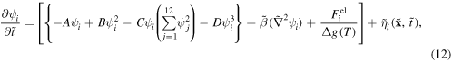
3. Evolution kinetics and material modeling
This section provides a brief description of the temperature dependent MPF evolution kinetics, phase transformation temperatures (martensite and austenite start and finish), and the thermo-mechanical material model of polycrystalline NiTi SMA at continuum level.
3.1. Phase fraction evolution
Phenomenological models based on extensive continuum level experimental data on thermally induced martensitic phase fraction have been proposed [8, 15, 42, 57–59]. Experiments are reported on annealed (at a temperature of 750 °C) polycrystalline austenite NiTi SMA (mainly [110] B2 crystal with weak [ 11] B2 crystal), with cooling and heating rate of 20 °C min−1, under various concentrations of Ni and Ti [42]. The model considered herein, essentially captures the kinetics of phase transformation rate as a function of phase fraction. It is assumed that, (a) the austenite transformation rate at any given temperature is proportional to the nucleation rate of austenite per unit volume and (b) the size of the austenite nucleus increases linearly with the austenite phase fraction. According to the model, the temperature dependent austenite phase fraction evolution is described through the Richards equation [42], i.e.

where  is the temperature dependent austenite phase fraction,
  the temperature of interest in K,
  the temperature corresponding to the maximum transformation rate, while
  and
and  (unitless) are the fit parameters which dictate the transformation or growth rate of the austenite phase. Equation (20) is adopted here to represent the martensitic phase fraction evolution as a function of temperature at coarse scales or continuum level. More details about this phenomenological model are available in [8, 15, 42, 57–59].
3.2. Thermo-mechanical continuum material model
The shape memory effect and super-elasticity are two paramount properties of SMAs, controlled by the thermo-mechanically induced austenite to martensite (and vice versa) phase transformation process. Above the austenite finish temperature  the SMA is in the austenite phase and upon loading it transforms into martensite and during unloading the martensite back transforms into austenite. Below
  depending on the temperature, the SMA leaves residual strain upon unloading which can be recovered by heating above
  In the process of loading–unloading, the SMA dissipates a large amount of energy through its flag-shaped hysteresis loop which again depends on the temperature and strain rate. Here the SMA material model of Helm and Haupt [60] is adopted, which has been verified experimentally and captures all essential aspects of the SMA behavior. The transformation temperatures considered here are those of NiTi SMA: (i) for the martensite start
  and finish
  temperatures are 295 and 275 K, respectively; (ii) for the austenite start
  and finish
  temperatures are 310 and 335 K, respectively. For uniaxial stress, it is expressed as


where,  is the developed stress, which depend on applied strain
  ambient temperature
  developed internal strain is
  Furthermore,
  is the developed internal strain rate,
  and
and  are the developed internal stress and its rate,
  and
and  are the MPF and its time rate and finally
  is the time rate of temperature evolution. Thus, the material model is expressed as a system of strongly nonlinear equations that need to be solved iteratively at every time step. For detailed description of the SMA material model and the iterative solution algorithm of those system of nonlinear equations i.e. equation (23). (a)–(e), the reader is referred elsewhere [8, 46, 60]. The hysteretic energy dissipation capacity of SMAs and its temperature modulation is addressed below.
4. Results and discussions
Previous experimental [9, 10, 17–19] as well as computational [8, 11, 13–15] studies at the nanometer scale demonstrate rather significant size effects on phase transformation kinetics of NiTi SMA. This section discusses the effect of length scale (shape and size) on the thermally induced phase evolution kinetics of NiTi thin samples. The effects of shape and size on the thermally induced phase fraction evolution kinetics is shown. Results at different length scale provide the basis for the multiscale coupling methodology of phase evolution kinetics in NiTi SMA. Next, the multiscale coupling results are used to improve the existing continuum material model of NiTi SMA.
4.1. Length scale effect on phase transformation kinetics for single crystals
Figure 1 shows MD simulations results on the effects of side length  and thickness
  of NiTi thin samples on the thermally induced MPF. To demonstrate the effect of side length
  the thickness of NiTi thin samples are kept constant i.e. for thickness
  To show the effect of thickness
  the side of the NiTi thin samples is given a constant value i.e.
  For each case, both of the austenitic (
 i.e. heating cycle) and martensitic (
 i.e. cooling cycle) thermally induced phase transformation process is shown, where, M and A are used to abbreviate the martensite and austenite phase, respectively. Figure 1(a) shows the effect of side length of NiTi thin samples on the temperature driven MPF curves for
  Similarly, figure 1(b) shows the effect of NiTi sample thickness on MPF evolution, for thickness
  with constant side length. It can be observed that during austenitic phase transformation, the effect of the simulation cell side length is almost the same for both the austenite start
  and finish
  temperatures, while in the MPT process, this effect is more pronounced in the martensite finish temperature
  than in the start temperature
  However, change in sample thickness causes a similar level of shift in the transformation temperatures (i.e. austenite and martensite start and finish).
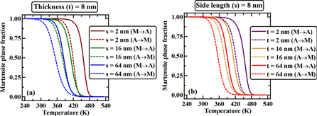
Figure 1. Effect of NiTi thin samples side length and thickness on the evolution of thermally induced martensite phase fraction (a) for constant thickness  with side length
  and (b) for constant side length
  with thickness
Download figure:
Standard image High-resolution imageSize effects are shown in figure 2, where both the side length and thickness of NiTi thin samples are changed proportionally, i.e.  and all three dimensions are increased proportionally from 2 to 64 nm; both heating and cooling cycles (i.e. austenitic and MPT process) are shown. Figure 2(a) shows the thermally induced MPF evolution curves for
  and figure 2(b) shows the same curves for
  It can be observed, at any temperature, with increasing size the MPF value decreases. Furthermore, the austenite start
  and martensite finish
  temperatures show more sensitivity to size than the austenite finish
  and martensite start
  temperatures. A discussion about the shape or the size effects in terms of the thermodynamics and available free surfaces is provided subsequently.
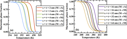
Figure 2. Size effect (variation of both thickness and side length) on the evolution of thermally induced martensite phase fraction in case of NiTi thin f samples (a) for  and (b) for
Download figure:
Standard image High-resolution imageAs discussed here, the length scale effects are attributed to the presence of the free surfaces, which are defects. The available free surface area per unit volume can be expressed as  Thus for any fixed thickness
  or side length
  the ratio of available free surface area per unit volume is
  or
or  with increasing
  or
or  this ratio quantity decreases inversely proportional to
  or
or  i.e.
i.e.  or
or  The presence of free surfaces changes the free energy density (energy per unit volume) of phase transformation. Assuming that energy reduces due to the presence of free surface area as
  (per unit surface), the drop in the free energy density is
  (per unit volume). Thus, increase in
  or
or  decreases the free energy density, which finally increases the total energy of the system. Therefore, to obtain similar level of phase transformation, more driving force is required with increasing
  or
or  In terms of thermodynamics, with increasing
  or
or  more temperature drop is required to obtain similar level of phase fraction. This ultimately shifts the phase evolution kinetics curves more towards low temperature and reduces the transformation temperature with increasing
  or
or 
Similarly to temperature dependent phase fraction evolution, length scales have a strong effect on the transformation temperatures (i.e. 


 and
and  ), as shown in figure 3. Figures 3(a1)–(c1) show the transformation temperatures associated with the austenitic (heating cycle) phase transformation process, while figures 3(a2)–(c2) shows the ones associated with the MPT process i.e. for cooling cycle. In every case, with increasing side length and thickness of the NiTi thin sample, the transformation temperature decreases. Figure 3(d) shows the effect of NiTi thin samples thickness and side length on the width of thermal hysteresis between the austenitic and MPT process, which represent the difference of temperature between the heating and cooling cycle for the same MPF. Interestingly, the width of the thermal cycle initially decreases with increasing thickness for samples of small side length. However, with increasing side length, this trend changes, i.e. the width of the thermal cycle initially decreases and after a critical thickness it increases. In every case, solid lines represent the shape effect, where only the side length changes while keeping the thickness constant. Whereas, the dotted line represents size effects, where both the side length and thickness of thin samples change. A nonlinear least-square minimization process on the data in figures 3(a1)–(c2) (through MATLAB 2014) shows a power law variation for the transformation temperatures with respect to side length. Thus, all of the phase transformation temperatures decrease with increasing side length, following a certain power law and the power law constant and exponent shows logarithmic variation with thickness, i.e. they decrease logarithmically with increasing thickness. In general, the transformation temperature model can be expressed as (i.e. as a function of
  and
and  )
)

where  (in nm) and
  (in nm) are constants, respectively, and
  (unitless) and
  (in nm) are constant for the power law exponent. Here,
  represents the shape and size dependency of the transformation temperatures i.e.


 and
and  and
and  represent the transformation temperatures associated with the bulk.
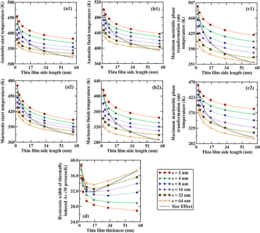
Figure 3. Effect of shape and size (i.e. both thickness and side length) on phase transformation temperatures and on thermal hysteresis width (a1) austenite start  (b1) austenite finish
  and (c1) maximum austenitic phase transformation rate temperature
  (a2) martensite start
  (b2) martensite finish
  and (c2) maximum martensitic phase transformation rate temperature
  (d) width of thermal cycle between austenitic and martensitic phase transformation process.
Download figure:
Standard image High-resolution imageA similar power law model of phase transformation temperature as the function of size has been proposed previously for other cases of nanostructures (such as for nanoparticles) [11, 13]. Those models, and the one proposed here, are only applicable at certain range of length scales, because any size below a critical length scale does not show phase transformation, as reported in [9–11, 13, 17–19]. In this context, Fu et al [9] reported that the growth of the surface oxide and its interfacial diffusion exert dominant constraining effects that produce high residual stress and low recovery capability. Experimental studies by Waitz et al [10, 17–19] show the effect of grain size and interaction of grain boundaries on the martensite phase transformation process due to the presence of nanograins for polycrystalline samples. The presence of grain boundaries and the interaction between grains play an important role in the evolution (nucleation and growth) and stabilization of different phases (B2 and B19' variants). In contrast to those studies, the present study, mainly shows results for single crystals (with crystal orientation of [110], [ 10], [001]) and thus any effect due to the residual stress or due the interaction between different crystals is not considered. However, to address the effect of grain size, grain boundaries, interaction between different grains and with the simulation cell size, PhF simulations for polycrystalline NiTi are performed. Also, an indirect method (based on the multiscale approach) is proposed to mimic the phase fraction evolution kinetics in polycrystalline NiTi. Here, the simulation results from different size single crystals i.e. the wavelet coefficients of MPF, for crystal orientation of [100], [110] and [111] are used in a unique way to reproduce the effects of polycrystals. Details about this are provided in section 4.4, for the polycrystalline NiTi case.
Therefore, it is important to note that, in the present study, the reported size effects are due to the presence of free surfaces, which act as defects and trigger phase transformation. With decreasing simulation cell size, the surface area per unit volume increases, and this creates the dependency of the phase transformation process (transformation temperatures and phase fraction) on size. Mutter and Nielaba [11] and Zhang et al [13] demonstrate the phase transformation process for single crystal nano-scale NiTi simulation cells, by employing an EAM potential similar to the one used in this study. Importantly, in the Zhang et al [13], it is found that below size (diameter) of 1.15 nm, no phase transformation occurs. In this study, the minimum size or side length of any simulation cell is adopted as 2.00 nm, which is above 1.15 nm. Finally, in the previous studies mentioned above, experiments and/or simulations are performed at constant temperature rates, which can play an important role in the phase transformation process, whereas in the present study quasi-static simulations (equilibrations) are performed at constant temperature. Thus, as potential future work, it will be very interesting to verify the model by employing experimental or simulation data for polycrystalline NiTi samples and obtain the model parameters.
4.2. Length scale effects on phase fraction and internal strain evolution in single crystals
The evolution of martensite phase faction and the development of internal strain in B19' due to the evolving martensite phase are the two most important quantities that govern the NiTi material model. Thus, it is important to accurately study the evolution of these two internal variables and transfer all relevant information to the continuum scales via multiscale coupling.
Figure 4 shows the length scale effects at the mesoscale and their linkage to microscale i.e. atomistic simulation results. At the mesoscale, 2D stochastic PhF simulation are performed and are linked to 3D atomistic (MD) simulations. For all MD simulations, the thickness  and a range of side lengths,
  is considered, with free boundary conditions in all directions. At the mesoscale level, the range of simulation cell sizes is from
  with free boundary conditions in all directions (x, y and z). Therefore, the side length cases of
  correspond to the MD and PhF overlap domain, where the two simulation methods are cross checked, showing very good agreement with each other. The error bars in the figures 4(a)–(c) are the results of uncertainty in the evolution of different phases (B2 and B19' variants). The uncertainty is quantified by performing a total of 25 Monte Carlo (MC) simulations at each temperature and for each size. In MD simulations, depending on the temperature, random velocities (based on Gaussian distribution) are provided to each atom and thus at the end of each simulation, the atomic coordinates are not the same as those obtained from other simulations at the same temperature and same size. Similarly at the beginning of stochastic PhF simulation, depending on the temperature, a Langevin noise term is added at every material point [7, 8]. This causes small but noticeable differences in the evolution of MPF, which ultimately produces uncertainties in the development of internal strain. Therefore, to account for those uncertainties, MC simulations are performed.
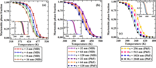
Figure 4. Evolution of martensite phase fraction with respect to temperature as a function of simulation cell size (a) within MD simulation domain, (b) within MD and PhF overlap simulation domain and (c) within PhF simulation domain.
Download figure:
Standard image High-resolution imageAnother important parameter is the internal strain in B19' that governs the stability of different phases (i.e. B2 and different variants of B19'). Since strong length scale effects are present in the phase evolution kinetics of NiTi (at both atomic and meso scales), it can be expected that similar effects should also be present for the transformation induced internal strain. However, this is not examined in the present work. In the MD simulations, the lattice parameters (bond lengths a, b and c, monoclinic bond angle β) of the B19' unit cell phase are measured. Here, it is important to mention that, in our MD simulations, with the adopted crystal orientation of B2 (i.e. [110], [ 10] and [001]) only two B19' variants are observed, which are favorable due to the requirement of low twining energy with respect to B2, as also reported in other MD studies [4, 8, 13–15] employing a similar interatomic potential. It is found from our MD simulations that, for the twin B19' unit cell, the twinning energy is
  with the difference in energy (i.e. the excess energy in reference to the single phase of B19') of
  which shows very good agreement with the values reported in the Zhong et al [4] study. Similarly, the twin boundary energy (i.e. the excess energy per unit boundary area of twin, in reference to the single phase of B19') is also estimated and found that its value is very small compared to the other B19' variants for the twining case, i.e.
  [4]. Finally, all of this indicates the possible reason for evolution of those two B19' variants, in our, as well as in other MD studies. Then, the deformation gradient matrix
  for the martensitic (B2 to any variants of B19') phase transformation is estimated based on the lattice parameters of the B19' unit cell phase and of the pristine B2 phase (a0). Since the lattice parameters of the B19' phase change with length scale
  and temperatures
 becomes a function of
  and
and  More information about
  for B2 → B19' phase transformation is available in previous studies [4, 25]. Next, to determine the transformation induced strain tensor of different variants of the B19' phase, the Green–Lagrange strain tensor
  for each of the variants is estimated as

Finally, knowing the fraction of B19' variants in the MD simulation cell (determined from the monoclinic bond angle β), at every temperature and for every size, the internal strain tensor in the B19' phase is estimated through

Now, the mean value of the internal strain tensor of the B19' phase  and associated uncertainty (standard deviation) are estimated from 25 MC MD simulations. Length scale effects in the average internal strain in the B19' phase is due to the differential fraction evolution among the different B19' variants. More information about the internal strain is provided in supplementary material. In PhF simulations, at any material point the internal strain associated with any B19' variant (
 for the ith field variable) [7, 26, 27] and its fraction (
 for the ith field variable), is used to estimate the total internal strain in B19' phase, as expressed trough
  (for the 12 variants). Here it is important to mention that, although during the simulation process the possibility of evolution of all 12 B19' variants is considered, only four B19' variants (1, 2, 6 and 8) are observed. It is due to the consideration of 2D simulation cell, as discussed in [8]. Interestingly, it is found here that for both MD and PhF simulations, the mean internal strain tensor
  is orthorhombic in nature. The mean value
  and its associated uncertainty is measured based on the number of MC simulations (here
  25) and number of material points
  in each simulation cell. Since the fractional evolution of B19' variants depends on the temperature and size of the simulation cell, the evolution of the average internal strain in the B19' phase is a function of temperature and simulation cell size. Next, from the mean internal strain tensors
  in the B19' phase, strains in three orthonormal directions (i.e.
 and
and  ) are shown in figure 5. This provides the direct estimation of temperature and size dependent lattice strains that B2 experiences during the MPT process. A recent relevant study by Ahadi and Sun [23] provides similar measures of lattice strains (in terms of stretches) and demonstrates the effect of grain size and applied strain on the evolution of lattice strain in NiTi SMA. As shown in figure 5, strong interplay between the average internal strain in B19' and the length scale of the simulation cell is present. With increasing length scale, a strong decay is observed in all components of the maximum value of the average internal strain in B19' i.e.
  It is clear that during the martensitic transformation process, the
 ![$[110]$](https://content.cld.iop.org/journals/0965-0393/25/4/045002/revision2/msmsaa6662ieqn260.gif) and
and ![$[001]$](https://content.cld.iop.org/journals/0965-0393/25/4/045002/revision2/msmsaa6662ieqn261.gif) directions of B2 experience compressive strain, while the
directions of B2 experience compressive strain, while the ![$[\bar{1}10]$](https://content.cld.iop.org/journals/0965-0393/25/4/045002/revision2/msmsaa6662ieqn262.gif) of B2 experiences tensile strain (as shown in figure 5(c)). Interestingly, for any length scale, the temperature dependency of the normalized
of B2 experiences tensile strain (as shown in figure 5(c)). Interestingly, for any length scale, the temperature dependency of the normalized  in B19' (normalized with respect to the maximum value i.e.
  ) follows the same Richard's equation as the one for the evolution kinetics of the MPF, i.e.

Figure 5. Evolution of average internal strains in B19' with respect to temperature as a function of simulation cell length scale (a)  in
in ![${[100]}_{{\rm{B}}19^{\prime} }$](https://content.cld.iop.org/journals/0965-0393/25/4/045002/revision2/msmsaa6662ieqn266.gif) or
or ![${[110]}_{{\rm{B}}2}$](https://content.cld.iop.org/journals/0965-0393/25/4/045002/revision2/msmsaa6662ieqn267.gif) direction, (b)
direction, (b)  in
in ![${[001]}_{{\rm{B}}19^{\prime} }$](https://content.cld.iop.org/journals/0965-0393/25/4/045002/revision2/msmsaa6662ieqn269.gif) or
or ![${[001]}_{{\rm{B}}2}$](https://content.cld.iop.org/journals/0965-0393/25/4/045002/revision2/msmsaa6662ieqn270.gif) direction and (b)
direction and (b)  in
in ![${[010]}_{{\rm{B}}19^{\prime} }$](https://content.cld.iop.org/journals/0965-0393/25/4/045002/revision2/msmsaa6662ieqn272.gif) or
or ![${[\bar{1}10]}_{{\rm{B}}2}$](https://content.cld.iop.org/journals/0965-0393/25/4/045002/revision2/msmsaa6662ieqn273.gif) direction; obtained from MD and PhF simulations.
direction; obtained from MD and PhF simulations.
Download figure:
Standard image High-resolution imageThe other components of internal strain tensor i.e.  and
and  does not follow a relation similar to equation (25). The relevant direct relation between the MPF and the internal strain tensor component
  implies that
  is mainly responsible for the stabilization of the B19' variants and B2. Using a fitting process, it is found that the different parameters of the evolution equation (equation (25)) i.e.
 and
and  vary with the length and can be expressed as


where  and
and  (unitless) are the constants corresponding to the bulk,
  is the temperature corresponding to the maximum martensite transformation rate of the bulk,
  (unitless) and
  (unitless) are constant for the power law exponent,
  (in nm),
  (in nm) and
  (in nm) are constants representing the length above which the length scale effect on
 and
and  is negligible, and
  and
and  represent the intercept and slop of the
  versus
  line.
line.
Since the off diagonal terms of the mean internal strain tensor are negligible, the diagonal terms furnish the principal components of the internal strain tensor. Interestingly, it is found that while the diagonal terms are only present in the mean value of the transformation induced total internal strain tensor of the B19' phase, the mean value of the total volumetric strain developed due to the MPT process (at any temperature and size) is almost zero, i.e. 
Figure 6 shows the effects of length scale on the phase transformation temperatures (martensite start, maximum transformation rate, and finish in figure 6(a)) and absolute maximum value of different elements of average internal strain tensor (i.e. 
 and
and  ) in B19' (in figure 6(b)). As can be observed from figure 6(a), all transformation temperatures decrease with increasing length scale, following a linear trend with log of the length scale i.e.
  Thus, each of the transformation temperatures can be described through an equation similar to equation (26c), where the slope of the line is the same yet the intercepts are different. Similarly to the transformation temperatures, the absolute maximum value of each of the components of the internal strain tensor in B19' phase decreases with length scale and can be expressed as
i.e. asymptotically converging to zero as size increases. Here,  (in %),
  (unitless) and
  (in nm) are constants.
Figure 6. Variation of the (a) martensite start  maximum martensitic transformation rate
  martensite finish
  temperature and (b) absolute maximum value of different components of the average internal strain in B19' (i.e.
 and
and  ) due to thermally induced martensitic phase transformation with respect to the simulation length scale. Empty and filled stars correspond to results from MD and PhF simulations, respectively, while the regression lines (solid or dotted lines) result from a fitting process.
Download figure:
Standard image High-resolution image4.3. Multiscale coupling of length scale effects
This section describes the multiscale/multiphysics coupling results for the thermally induced phase transformation process. Multiscale coupling via the CWM methodology is performed on the MPF evolution. Here, the statistical information of length scale effects on the MPF evolution kinetics (obtained via MD and PhF simulations), is transferred/propagated from micro and meso scales to the macro scale. Furthermore, the CWM results are compared with continuum level experimental data and with macroscopic constitutive relations for NiTi SMA. Essentially, the continuum level experimental data/evolution law predicts an exponential dependency of MPF evolution on temperature, while the macroscopic constitutive relations are linear. Therefore, in this section, the experimental data is referred to as the 'exponential' model and MPF obtained from macroscopic constitutive relations is referred as the 'linear' model.
Figure 7 demonstrates the ability of the CWM method to transfer the trend and uncertainties of MPF to the continuum level. In this context, it is important to noted that, the experimental sample is the polycrystalline with mostly contain [110] B2 crystals, i.e. similar like the CWM simulations. Thus, it can be expected that, in the CWM method, the effect of the grain boundary energy and internal strain, on the MPF evolution is captured sufficiently, as is the case for the experiments. Figure 7(a) shows the evolution of MPF as a function of temperature predicted by the CWM method, experimental data, described above in section 3.1, and from the continuum level thermo-mechanical constitutive relation (mentioned in section 3.2). It can be observed that the evolution of MPF predicted by the CWM method matches very well the experimental data/exponential model i.e. the blue curve [8, 42]. Also, the CWM method transfers the statistics of length scale effects, as shown in figure 7(a), in terms of the uncertainty bars on the CWM curve. However, the continuum level linear material model shows significant deviation from the experimental and/or CWM results. To demonstrate the deviation, the differences between values from experimental data and from CWM and continuum material model are shown in figure 7(b). The difference between experimental data/exponential model and CWM predicted values is small or even negligible when uncertainties are considered, whereas this difference becomes very large for the case of experimental data and linear model obtained from continuum level thermo-mechanical constitutive relations.
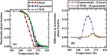
Figure 7. Variation of the (a) martensite phase fraction and (b) difference in martensite phase fraction with respect to the temperature, from different sub methods and material model. In figure 7(a), the blue curve (exponential) represents the experimental data [8, 42] and the red curve (linear) the one from macroscopic constitutive relations.
Download figure:
Standard image High-resolution image4.4. Multiscale modeling and length scale and grain size effects in NiTi polycrystals
The interplay of cell/specimen size and grain size on the thermo-mechanical properties such as phase transformation process in SMAs has received little attention despite its importance [16], perhaps because of the difficulties in addressing it. In some recent studies [1, 21–23], attempts are made to model or experimentally demonstrate the effect of grain size on stress induced MPT (i.e. for superelasticity) in NiTi SMA. However, the interaction between sample size and grain size and their coupled effects on the MPT process was addressed in those studies. Therefore, differing from the previous studies [1, 21–23], in this study, some attempts are made to shed the light on the effect of such interplay. Here, 2D PhF simulations are used to address the interplay of simulation cell size and grain size on the thermally induced MPF evolution, while for the multiscale modeling, simulation results (of different size single crystal) from both MD and PhF are adopted, as discussed subsequently.
In order to perform PhF simulation of polycrystalline NiTi, simulation cells with the polycrystalline grain boundaries or interfaces are generated via Poisson–Voronoi tessellations, employing the MATLAB toolbox. To introduce the effect of grain boundary a gradient energy term is added, as mentioned in the Ahluwalia et al study [16]. This gradient energy term is expressed as the function of interfacial energy  width of the grain boundary
  and field variable
  The value of the interfacial energy term
  for all different type of interfaces (such as interface between all B2 and B19' crystals, as well as B2-B19' interface) is considered the same, as assumed in other studies [7, 16]. However, the effect of different B2 crystal orientation on the MPF evolution is incorporated in the PhF model through the elastic strain energy term [7, 8, 16]. This elastic strain energy depends on the transformation strain tensors for B2 to B19' variants
  which again depends on the crystal orientation (with respect to [100] B2 crystal) [7, 8, 16]. Therefore, before using those transformation strain tensors, they are rotated through the rotation matrix
  i.e.
i.e.  is converted into
  [7, 8, 16]. Here, this rotation matrix depends on the crystal orientation of a particular B2 grain, with respect to the [100] B2 crystal. Thus, based on the aforementioned process, the effects of interface/grain boundary and crystal orientation are incorporated in the PhF model.
An indirect method (based on the multiscale approach) is used to mimic the results of polycrystalline NiTi SMA. For that, the wavelet coefficients of MPF from different size single crystal simulations (with the crystal orientation of [100], [110] and [111]) are used in a very unique way. Here, to construct the coefficients of the CWM of the polycrystalline NiTi, wavelet coefficients of different single crystal NiTi are fused from different length scales, i.e. from different size samples. In case of single crystals (with orientations [100], [110] and [111]), depending on the size of the cells, simulations are performed employing MD and PhF, as mentioned in section 2. It is important to mention that, before mixing the wavelet coefficients (obtained from different size single crystals of NiTi), they are multiplied by appropriate weight factors. These weight factors are adopted based on the fraction of the relevant crystal present in the simulation cell. Adopting these weight factors is important, since they act as a step up or step down operator and thus amplify or reduce the value of the wavelet coefficients of single crystal NiTi, such that similar (to a close approximation) wavelet coefficients of polycrystalline NiTi are obtained. Since, in this indirect method the CWM is constructed, it is referred to as the 'Hybrid CWM' and this term is used subsequently.
To demonstrate the coupled effect of grain size and length scale on MPF evolution and its associated multiscale modeling, a simulation cell of size  nm is adopted and simulations are performed at four different temperatures (T = 300, 313, 325 and 350 K) with different grain sizes. Figure 8 shows the effect of grain size on the thermally induced MPF evolution, for simulation cell size
  nm. The average values of the grain size and corresponding MPF are directly plotted in figure 8, while their corresponding uncertainties are represented through the error bars. In order to directly compare the single crystal and polycrystal simulations, MPF values (mean and standard deviation) are provided for the four different temperatures. Figure 8(a) shows the coupled effects of grain size and simulation cell size, on the thermally induced MPF evolution, at T = 313 K. Also, figure 8(a) demonstrates the efficiency of the hybrid CWM method in mimicking the MPF evolution of polycrystalline NiTi SMA as a function of grain size, for T = 313 K. It is seen that the MPF obtained from the direct polycrystal 2D PhF simulations and the hybrid CWM method are in very good agreement with each other. Further, those results are compared with a reported computational study [16] and an experimental study [42]. Results from the computational study [16] agree very well with our direct polycrystalline NiTi simulation, as well as with the hybrid CWM predictions. However, the experimental value stays a little off from all other cases. Such deviation can be attributed to size effects for the NiTi samples/cells and due to the constant temperature simulation. The experiments [42] were conducted at the continuum level, with a fixed temperature rate (20 °C min−1 cooling and heating rate).
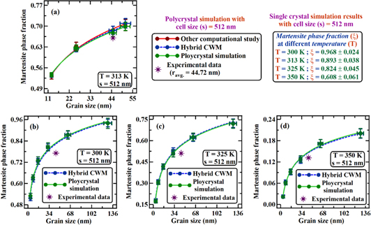
Figure 8. Variation of martensite phase fraction as a function of grain size for polycrystalline simulation cell of size  nm, at temperature (a)
  (b)
(b)  (c)
(c)  and (d)
  Other study result (computational study for the polycrystalline NiTi) and experimental data are from the [16, 42], respectively. Deviation between experiments and simulations is attributed to size effects as discussed in the text.
Download figure:
Standard image High-resolution imageNext, to conform and emphasize the efficiency and prediction capability of the hybrid CWM method, results are generated at different temperatures (T = 300, 325 and 350 K) and compared to the direct simulation results of polycrystalline NiTi SMA. As shown in figures 8(b)–(d), the hybrid CWM results agree very well with the direct polycrystalline simulation results. Further, the deviation of the experimental MPF values from the simulation ones (from both the direct simulation and hybrid CWM) decreases with increasing temperature. For all examined temperatures, when the results from polycrystalline NiTi are compared to the results from single crystal NiTi, a significant difference in the MPF value is observed. Such noticeable difference in MPF value arises from the presence of grain boundary. Further, the simulations confirm that with the reduction in grain size, the evolution of the MPF decreases drastically and thus below a critical grain size MPT will not be observed in case of the polycrystalline NiTi SMA, as reported in many other studies [1, 10, 17–19, 21–23].
The above results show the coupled effect of grain size and simulation cell size on thermally induced MPF evolution, but do not clearly show the interplay between grain size and cell size and their effect on the MPF evolution. Figure 9 shows such interplay for three different temperatures (T = 300, 325 and 350 K), the interplay becoming prominent for smaller grain sizes. To clearly investigate the interplay, direct polycrystalline PhF simulations are performed. For each temperature (and mainly for T = 300 and 325 K), with the increase in simulation cell size (i.e. removal of length scale effects), the grain size effect becomes more pronounced, causing a drastic decrease in MPF evolution with decrease in grain size. This can be explained as follows. For larger simulation cell with smaller grain size, the effective amount (length) of grain boundary is high, which increases the total grain boundary energy. High grain boundary energy provides a driving force opposing the MPT process and thereby prevents the nucleation and growth of martensite (different variants of B19') from austenite (B2). Interestingly, it can be observed that with the increase in simulation cell size, as the length scale effect is removed, polycrystalline NiTi simulation results start agreeing very well with experimental data. To further demonstrate the effect of grain size in polycrystalline NiTi, results of single crystal NiTi simulations are also shown in figure 9. Finally, the relation between normalized MPF and normalized grain size can be express as

where,  and
and  are the MPFs corresponding to polycrystalline and single crystal NiTi SMA, respectively,
  and
and  are the grain size and simulation cell size, respectively,
  is a unitless constant which represent the normalized MPF value for a sample with very large grain size, and
  is a constant representing the normalized MPF and normalized grain size (in log scale) curve.

Figure 9. Variation of martensite phase fraction as a function of grain size for polycrystalline simulation cell of size  nm, shows the interplay of grain size and the simulation cell size on martensite phase fraction evolution, at temperature (a)
  (b)
(b)  and (c)
Download figure:
Standard image High-resolution image4.5. Stress–strain response
This section describes the application of multiscale coupling to macroscopic continuum scale constitutive relations. In order to improve the continuum thermo-mechanical material model of NiTi SMA described previously, the temperature dependent MPF and its spatial uncertainties (obtained from multiscale coupling) are transferred into the continuum constitutive model. In the present version of the continuum model it is assumed that the MPF varies linearly with temperature.
Figure 10 shows the stress strain hysteretic loops and the associated energies obtained from different methods and from experimental data. The linear evolution law for the thermally induced MPF shows noticeable deviation from the experimental stress–strain data, while the exponential evolution law (expressed in equation (20)) and the CWM provided thermally induced MPF show very good agreement with the experimental data. The same holds for energy dissipation capacity of NiTi SMA (figure 10(b) for single cycle and figure 10(c) for multiple cycles). Thus, the improvement in the material modeling of NiTi SMA is rather significant, at least for those cases where NiTi SMA is used as an energy dissipative medium, such as in NiTi SMA based vibration dampers or actuators.

Figure 10. (a) Stress strain hysteresis loop of NiTi at T = 300 K obtained by employing different methods and experimental data. Comparison of hysteresis energy dissipation capacity at various temperatures (b) in single cycle and (c) in multiple cycles.
Download figure:
Standard image High-resolution imageThe improvement in the continuum material model is demonstrated for other temperature cases in figure 11. It can be observed that within the transformation temperature zone, the stress–strain hysteresis loops obtained from the linear evolution law deviates from that obtained from CWM and from exponential evolution law. However, outside the transformation temperature regime, such differences in the stress–strain hysteresis loops diminish. Here at T = 200 K, the MPF obtained from different models is the same, thus in figure 11(a) stress–strain hysteresis loop obtained from different models are indistinguishable.

Figure 11. Constitutive behavior of the NiTi SMA at different temperatures obtained from different methods.
Download figure:
Standard image High-resolution imageThe uncertainties associated with thermally induced MPF obtained from the multiscale coupling are used to demonstrate the hysteretic stress–strain response of NiTi SMA at different temperatures. In figure 12, for each temperature, five curves are plotted, i.e. at mean phase fraction value and at mean with two different levels of uncertainties  It can be observed that within the transformation temperature regime, uncertainty in the thermally induced MPF has a pronounced effect on the stress–strain response. However, this effect of uncertainties diminishes outside the transformation temperature zone.
Figure 12. Effect of uncertainties in the thermally induced martensite phase fraction on the stress–strain response of NiTi SMA at different temperatures.
Download figure:
Standard image High-resolution image
5. Conclusions
This study demonstrates the effects of length scale (i.e. shape and size effects) on thermally induced MPF evolution kinetics in NiTi SMA and implements a relevant multiscale and multiphysics model. To study the evolution kinetics of B2 and of B19' variants, different methods, MDs simulations for fine scale, PhF simulations for meso scale, and experimental data for continuum level, are used. The LBM is employed for simulating the heat diffusion process in NiTi thin samples and multiscale coupling is performed through the CWM method. Results of this study show strong length scale effects, which are linked to the presence of free surfaces. Change of size and shape of NiTi thin samples causes substantial changes in the transformation temperatures, as well as in the width of thermal cycles. With increasing side length and thickness of the thin sample, the transformation temperatures decrease. The temperature dependent evolution of MPF follows the phenomenological Richard's equation. Strong length scale effects are also noticed for the evolution kinetics of the average internal strain in the B19' phase, and its maximum value decreases exponentially with increasing simulation cell size. Interestingly, it is found that, the same Richard's equation can be used to express the temperature dependency of the normalized average internal strain in the B19' phase. Through multiscale coupling, the length scale effects on thermally induced MPF evolution and its associated uncertainties are propagated into the continuum level and used to improve existing constitutive models for NiTi SMA. The efficiency and robustness of the multiscale modeling method is further demonstrated for polycrystalline NiTi samples at different temperatures, and shows the coupled effects of grain size, simulation cell size, and temperature on the MPF evolution kinetics. The interplay between grain size and length scale on the thermally induced MPF evolution shows that for large simulation cell size (where the length scale effect is negligible) and small grain size, the MPT process arrests. The effect becomes more pronounced for large size simulation cells, where, with decreasing grain size, the MPF decreases drastically. Employing the multiscale modeling results, the continuum level thermo-mechanical constitutive relation is modified appropriately. The modified material model significantly improves the predicted stress–strain response and energy dissipation capacity of NiTi SMA and shows good agreement with experimental data. Furthermore, the uncertainties in MPF evolution show noticeable effects in the macroscopic stress–strain response. It can be concluded that improvement in material model and consideration of such uncertainties are important, at least for designing NiTi SMA base devices such as dampers and actuators. In future work, it will be interesting to study the interplay of grain size in polycrystalline NiTi SMA and cell size in the evolution kinetics (nucleation and growth of different phases) and their effect on phase transformation temperatures.
Acknowledgments
The reported exploratory work became possible through the support of SG by the University of Arizona. Also the authors would like to acknowledge Prof Ting Zhu (from Woodruff school of mechanical engineering at Georgia Institute of Technology) for providing the interatomic potential parameters.