Exact computation of projected sphere centres in cone beam x-ray projections

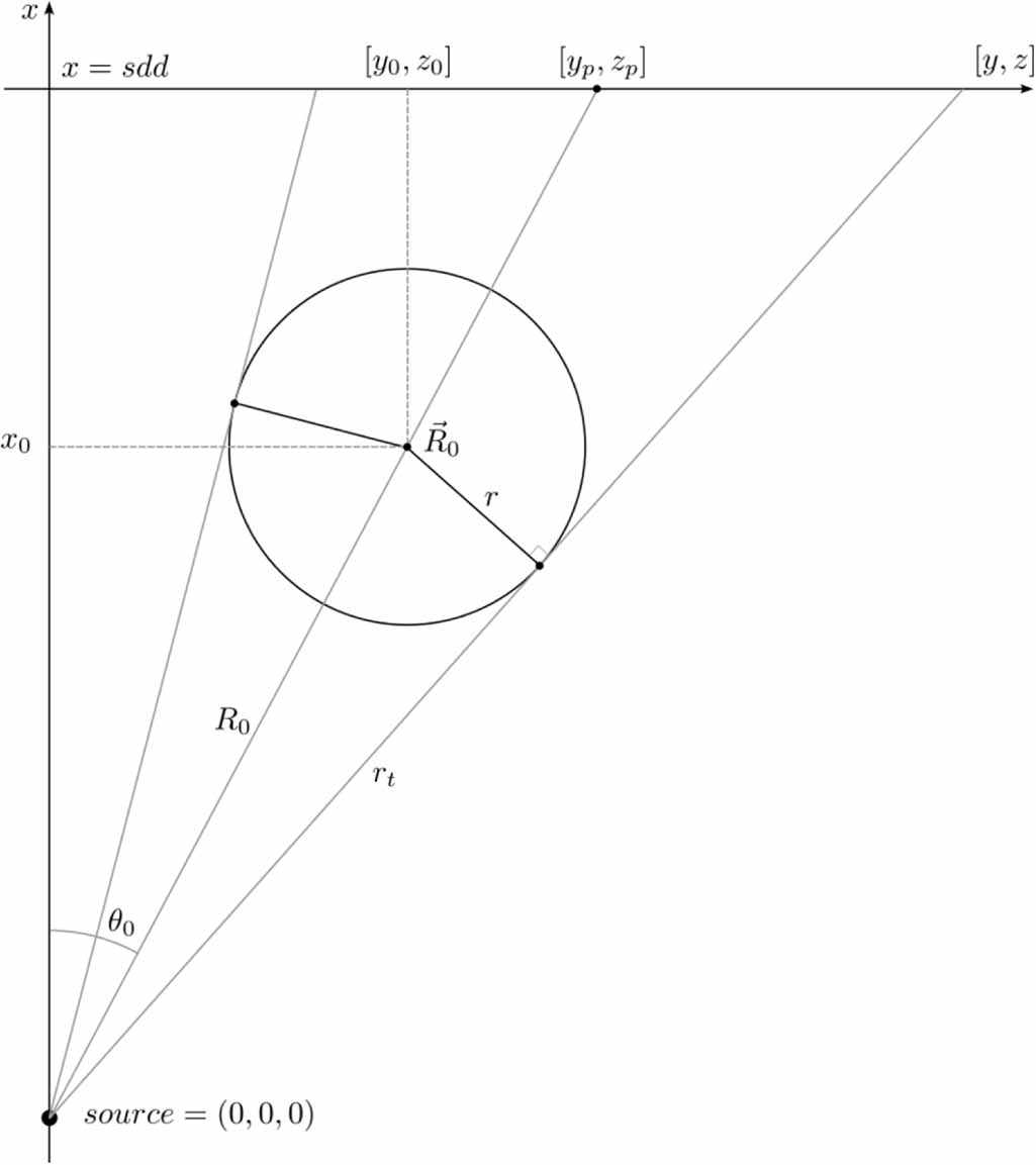
For the description of the sphere projection geometry, we define a coordinate system with an ideal (point-like) x-ray source at the origin and a detector in the plane perpendicular to the x-axis at coordinate $x = sdd$ (source detector distance). An ideal sphere of radius $r$ is placed at coordinates ${\overset{{\scriptscriptstyle\rightharpoonup}} {R} _0} = \left( {{x_0},{y_0},{ }{z_0}} \right)$ with ${x_0} > 0$ and ${R_0}: = | {{{\overset{{\scriptscriptstyle\rightharpoonup}} {R} }_0}} | = \sqrt {x_0^2 + y_0^2 + z_0^2}$ as depicted in figure 1. Due to the symmetry of a sphere, the projection of the sphere edge must be described by a cone that is tangential to the sphere and has its apex at the origin (x-ray source). The intersection of this tangent cone with the sphere edge must be a circle and all points on this circle have the same distance ${r_t} = \sqrt {R_0^2 - {r^2}}$ from the origin.

Zoom In Zoom Out Reset image size

The points on the tangent circle must therefore satisfy 2 equations for the distance from the sphere centre and from the origin:

$$\begin{align}{r^2} &= {\left( {x - {x_0}} \right)^2} + {\left( {y - {y_0}} \right)^2} + {\left( {z - {z_0}} \right)^2}\end{align} \tag{ 1 }$$

$$\begin{align}r_t^2 &= {x^2} + {y^2} + {z^2} = R_0^2 - {r^2} = x_0^2 + y_0^2 + z_0^2 - {r^2}.\end{align} \tag{ 2 }$$

Equation (2) can be rewritten as

$$\begin{equation}{x_0} = \sqrt {r_t^2 + {r^2} - y_0^2 - z_0^2} .\end{equation} \tag{ 3 }$$

For bringing the tangent circle equation into a usable form, we use a coordinate system that we call directional coordinates and define as

$$\begin{align} R: &= \sqrt {{x^2} + {y^2} + {z^2}} \nonumber\\ \eta : &= \frac{y}{R} = \frac{y}{{\sqrt {{y^2} + {z^2}} }}\frac{{\sqrt {{y^2} + {z^2}} }}{R} = \cos \varphi \sin \theta \nonumber\\ \zeta : &= \frac{z}{R} = \frac{z}{{\sqrt {{y^2} + {z^2}} }}\frac{{\sqrt {{y^2} + {z^2}} }}{R} = \sin \varphi \sin \theta \end{align} \tag{ 4 }$$

where the definition of the angles $\varphi ,\theta \,$ shown in figure 2 is not necessary but illustrates the link to the more commonly used spherical coordinates.

Zoom In Zoom Out Reset image size

The purpose of this choice is that any point of the sphere and its projection onto the detector have the same $\eta ,\zeta$ coordinates in this coordinate system.

An illustration of the conversion of a circle and an ellipse in Cartesian coordinates to directional coordinates is shown in figure 3.

Zoom In Zoom Out Reset image size

Cartesian coordinates are expressed in directional coordinates as

$$\begin{align} y &= R \cdot \eta \nonumber \\ z &= R \cdot \zeta \nonumber \\ x &= \sqrt {{R^2} - {y^2} - {z^2}} = R\sqrt {1 - {\eta ^2} - {\zeta ^2}} .\end{align} \tag{ 5 }$$

And therefore

$$\begin{equation}R = \frac{x}{{\sqrt {1 - {\eta ^2} - {\zeta ^2}} }}.\end{equation} \tag{ 6 }$$

Expressing equation (1) in directional coordinates and applying equation (3) yields

$$\begin{align}{r^2} &= {\left( {R\sqrt {1 - {\eta ^2} - {\zeta ^2}} - \sqrt {r_t^2 + {r^2} - y_0^2 - z_0^2} } \right)^2} + {\left( {R\eta - {y_0}} \right)^2} \nonumber \\ &\quad + {\left( {R\zeta - {z_0}} \right)^2}.\end{align} \tag{ 7 }$$

Using the fact that $R = {r_t}$ for all points of the tangent circle and dividing by $r_t^2$, equation (7) becomes

$$\begin{align} {\left( {\frac{r}{{{r_t}}}} \right)^2} &= {\left( {\eta - \frac{{{y_0}}}{{{r_t}}}} \right)^2} + {\left( {\zeta - \frac{{{z_0}}}{{{r_t}}}} \right)^2} + \left(\sqrt {1 - {\eta ^2} - {\zeta ^2}} \right.\nonumber\\ &\quad \left.- \sqrt {1 + {{\left( {\frac{r}{{{r_t}}}} \right)}^2} - {{\left( {\frac{{{y_0}}}{{{r_t}}}} \right)}^2} - {{\left( {\frac{{{z_0}}}{{{r_t}}}} \right)}^2}} \right)^2 .\end{align} \tag{ 8 }$$

Equation (8) describes in directional coordinates both the cone tangent circle of a sphere and the edge of the sphere's projection on the detector with 3 fit parameters

$$\begin{equation*}\frac{r}{{{r_t}}},\,\frac{{{y_0}}}{{{r_t}}},\frac{{{z_0}}}{{{r_t}}}.\end{equation*}$$

These parameters do not yet correspond to the sphere centre in directional coordinates, but they can be converted using the relation

$$\begin{equation}\frac{{{r_t}}}{{{R_0}}} = \frac{{{r_t}}}{{\sqrt {r_t^2 + {r^2}} }} = \frac{1}{{\sqrt {1 + {{\left( {\frac{r}{{{r_t}}}} \right)}^2}} }}.\end{equation} \tag{ 9 }$$

The sphere centre in directional coordinates and the sphere radius relative to the sphere distance from the origin are therefore obtained as

$$\begin{equation}\begin{aligned} \frac{{{y_0}}}{{{R_0}}} &= \frac{{{y_0}}}{{{r_t}}} \cdot \frac{{{r_t}}}{{{R_0}}} = \frac{{{y_0}}}{{{r_t}}} \cdot \frac{1}{{\sqrt {1 + {{\left( {\frac{r}{{{r_t}}}} \right)}^2}} }} \\ \frac{{{z_0}}}{{{R_0}}} &= \frac{{{z_0}}}{{{r_t}}} \cdot \frac{{{r_t}}}{{{R_0}}} = \frac{{{z_0}}}{{{r_t}}} \cdot \frac{1}{{\sqrt {1 + {{\left( {\frac{r}{{{r_t}}}} \right)}^2}} }} \\ \frac{r}{{{R_0}}} &= \frac{r}{{{r_t}}} \cdot \frac{{{r_t}}}{{{R_0}}} = \frac{r}{{{r_t}}} \cdot \frac{1}{{\sqrt {1 + {{\left( {\frac{r}{{{r_t}}}} \right)}^2}} }} \end{aligned} .\end{equation} \tag{ 10 }$$

From the directional coordinates of the sphere centre, the Cartesian coordinates $[{x_p},{y_p},{z_p}]$ of the sphere centre projection can be calculated from equations (5) and (6) as

$$\begin{equation}\begin{aligned} {x_p} &= sdd \\ {y_p} &= \frac{{{y_0}}}{{{R_0}}} \cdot \frac{{sdd}}{{\sqrt {1 - {{\left( {\frac{{{y_0}}}{{{R_0}}}} \right)}^2} - {{\left( {\frac{{{z_0}}}{{{R_0}}}} \right)}^2}} }} \\ {z_p} &= \frac{{{z_0}}}{{{R_0}}} \cdot \frac{{sdd}}{{\sqrt {1 - {{\left( {\frac{{{y_0}}}{{{R_0}}}} \right)}^2} - {{\left( {\frac{{{z_0}}}{{{R_0}}}} \right)}^2}} }} \\ \end{aligned} \end{equation} \tag{ 11 }$$

and analogously, the sphere radius magnified to $sdd$ is

$$\begin{equation}{r_p} = \frac{r}{{{R_0}}} \cdot \frac{{sdd}}{{\sqrt {1 - {{\left( {\frac{{{y_0}}}{{{R_0}}}} \right)}^2} - {{\left( {\frac{{{z_0}}}{{{R_0}}}} \right)}^2}} }}.\end{equation} \tag{ 12 }$$

For fitting the projection of a sphere with equation (8) in directional coordinates using the coordinate transformation in equation (4), the detector pixel grid first has to be converted into Cartesian coordinates as described in the following section.

Note that while a general fit of an ellipse (as the general shape of a sphere projection) in a detector image uses 5 fit parameters (centre y and z coordinates, major and minor axes, orientation angle), equation (8) appears to have only 3 degrees of freedom. The 2 missing parameters are 'hidden' in the coordinate system and given by the pixel coordinates $\left[ {{u_0},{v_0}} \right]$ where the x-ray beam is perpendicular to the detector plane, defined as the intersection of the x-axis with the detector plane in Cartesian coordinates ($y = z = 0$) in figure 1. In a conventional, well-aligned x-ray imaging setup, this perpendicular pixel will normally be close to the detector centre, but it can deviate from the centre in general.

Using the pixel size (side length) ${d_{px}}$ for a given detector and the sign convention defined in figure 2, the conversion from image pixel coordinates $\left[ {u,\,v} \right]$ to Cartesian coordinates of the imaging setup (as defined in figure 1) is given by

$$\begin{equation}\begin{aligned} x &= sdd \\ y &= - \left( {u - {u_0}} \right) \cdot {d_{px}} \\ z &= - \left( {v - {v_0}} \right) \cdot {d_{px}} \end{aligned} .\end{equation} \tag{ 13 }$$

Conversely, the pixel coordinates $\left[ {{u_p},{v_p}} \right]$ of the projected sphere centre are obtained as

$$\begin{equation}\begin{aligned} {u_p} = - \frac{{{y_p}}}{{{d_{px}}}} + {u_0} \\ {v_p} = - \frac{{{z_p}}}{{{d_{px}}}} + {v_0} \end{aligned} .\end{equation} \tag{ 14 }$$

For an x-ray projection image containing $n$ (spatially separated) spheres, fitting all sphere projections with ellipses requires $5n$ fit parameters (or $4n + 2$ if the orientation of the ellipses is restricted to point towards the image centre). The method described here, however, only requires $3n + 2$ parameters, since the orientation of the detector with respect to the x-ray beam is independent of the number or position of spheres that are placed in the cone beam and the eccentricity of the projection ellipse is incorporated in the coordinate system.

Using a projection of multiple spheres (or multiple projections of variable sphere positions with fixed detector orientation) can therefore allow for fitting the perpendicular pixel coordinates $\left[ {{u_0},{v_0}} \right]$ from the shapes of the projected spheres without knowing the actual sphere positions or diameters.

In some cases, it may be more convenient to model the position of the edge of a sphere projection rather than its centre. For instance, if the projection of a sphere is overlapped by some sort of support structure to one side of the sphere, fitting the edge pixels on the support side will be inaccurate or unstable and influence the fitted sphere centre, but the edge pixels on the clear side may still be fitted accurately.

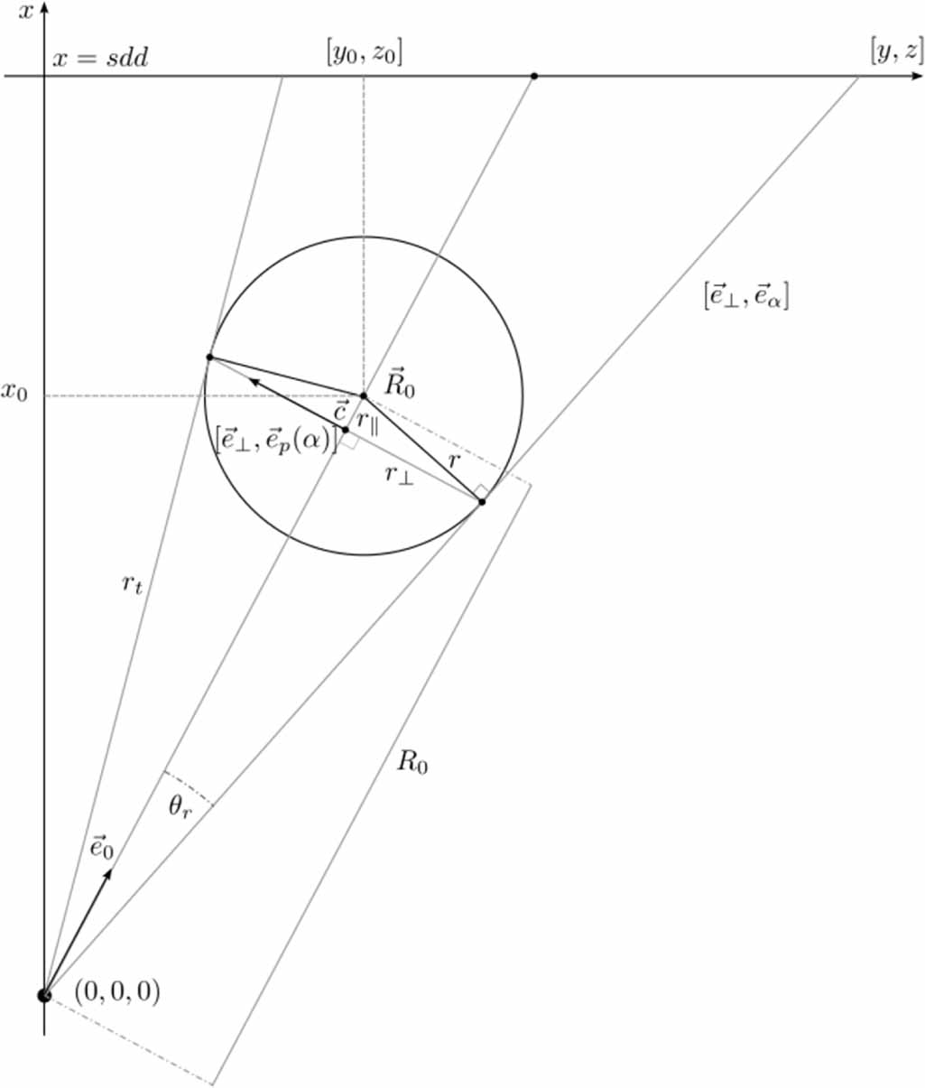
In order to be able to model the edge of a sphere projection with subpixel resolution, a parametrization of the tangent circle of the sphere was derived.

Using geometric similarity (or trigonometric identities and the half cone angle ${\theta _r}$) in figure 4, it can be seen that

$$\begin{equation}\begin{aligned} \frac{{{r_ \bot }}}{r} &= \frac{{{r_t}}}{{{R_0}}} = \frac{1}{{\sqrt {1 + {{\left( {\frac{r}{{{r_t}}}} \right)}^2}} }} \\ \frac{{{r_\parallel }}}{r} &= \frac{r}{{{R_0}}} = \frac{r}{{{r_t}}} \cdot \frac{1}{{\sqrt {1 + {{\left( {\frac{r}{{{r_t}}}} \right)}^2}} }} \end{aligned}. \end{equation} \tag{ 15 }$$

Zoom In Zoom Out Reset image size

And using equations (9) and (10)

$$\begin{equation}\begin{aligned} \frac{{{r_ \bot }}}{{{r_t}}} &= \frac{{{r_ \bot }}}{r} \cdot \frac{r}{{{r_t}}} = \frac{{\frac{r}{{{r_t}}}}}{{\sqrt {1 + {{\left( {\frac{r}{{{r_t}}}} \right)}^2}} }} \\ \frac{{{r_\parallel }}}{{{r_t}}} &= \frac{{{r_\parallel }}}{r} \cdot \frac{r}{{{r_t}}} = \frac{{{{\left( {\frac{r}{{{r_t}}}} \right)}^2}}}{{\sqrt {1 + {{\left( {\frac{r}{{{r_t}}}} \right)}^2}} }} \end{aligned} .\end{equation} \tag{ 16 }$$

The unit vector ${\overset{{\scriptscriptstyle\rightharpoonup}} {e} _0}$ pointing from the origin to the sphere centre ${\overset{{\scriptscriptstyle\rightharpoonup}} {R} _0}$ can be expressed in directional coordinates of the sphere centre:

$$\begin{align}{\overset{{\scriptscriptstyle\rightharpoonup}} {e} _0} &= \frac{{{{\overset{{\scriptscriptstyle\rightharpoonup}} {R} }_0}}}{{{R_0}}} = \frac{1}{{{R_0}}}\left( {\begin{array}{*{20}{c}} {{x_0}} \\ {\begin{array}{*{20}{c}} {{y_0}} \\ {{z_0}} \end{array}} \end{array}} \right) = \frac{1}{{{R_0}}}\left( {\begin{array}{*{20}{c}} {\sqrt {R_0^2 - y_0^2 - z_0^2} } \\ {\begin{array}{*{20}{c}} {{y_0}} \\ {{z_0}} \end{array}} \end{array}} \right) \nonumber\\ &= \left( {\begin{array}{*{20}{c}} {\sqrt {1 - {{\left( {\frac{{{y_0}}}{{{R_0}}}} \right)}^2} - {{\left( {\frac{{{z_0}}}{{{R_0}}}} \right)}^2}} } \\ {\begin{array}{*{20}{c}} {\frac{{{y_0}}}{{{R_0}}}} \\ {\frac{{{z_0}}}{{{R_0}}}} \end{array}} \end{array}} \right).\end{align} \tag{ 17 }$$

An arbitrary unit vector ${\overset{{\scriptscriptstyle\rightharpoonup}} {e} _ \bot }$ perpendicular to ${\overset{{\scriptscriptstyle\rightharpoonup}} {e} _0}$ can without loss of generality be chosen to have 0 z-component, i.e.

$$\begin{equation}{\overset{{\scriptscriptstyle\rightharpoonup}} {e} _ \bot } = \frac{1}{{\sqrt {e_{ \bot ,x}^2 + e_{ \bot ,y}^2\,} }}\left( {\begin{array}{*{20}{c}} {{e_{ \bot ,x}}} \\ {\begin{array}{*{20}{c}} {{e_{ \bot ,y}}} \\ 0 \end{array}} \end{array}} \right).\end{equation} \tag{ 18 }$$

From the requirement of orthogonality,

$$\begin{equation}\begin{gathered} {{\overset{{\scriptscriptstyle\rightharpoonup}} {e} }_ \bot } \cdot {{\overset{{\scriptscriptstyle\rightharpoonup}} {e} }_0} = 0 = {e_{ \bot ,x}}{e_{0,x}} + {e_{ \bot ,y}}{e_{0,y}} \\ \Leftrightarrow = {e_{ \bot ,x}} = - \frac{{{e_{0,y}}}}{{{e_{0,x}}}}\,{e_{ \bot ,y}} = : - {p_0}\,{e_{ \bot ,y}} \\ \end{gathered} .\end{equation} \tag{ 19 }$$

With

$$\begin{equation}{p_0} = \frac{{{e_{0,y}}}}{{{e_{0,x}}}} = \frac{{\frac{{{y_0}}}{{{R_0}}}}}{{\sqrt {1 - {{\left( {\frac{{{y_0}}}{{{R_0}}}} \right)}^2} - {{\left( {\frac{{{z_0}}}{{{R_0}}}} \right)}^2}} }}.\end{equation} \tag{ 20 }$$

Since ${\overset{{\scriptscriptstyle\rightharpoonup}} {e} _ \bot }$ was defined with a normalization factor, we can choose ${e_{ \bot ,y}} = 1$ and obtain

$$\begin{equation}{\overset{{\scriptscriptstyle\rightharpoonup}} {e} _ \bot } = \frac{1}{{\sqrt {1 + p_0^2\,} }}\left( {\begin{array}{*{20}{c}} { - {p_0}} \\ {\begin{array}{*{20}{c}} 1 \\ 0 \end{array}} \end{array}} \right).\end{equation} \tag{ 21 }$$

This orthogonal vector ${\overset{{\scriptscriptstyle\rightharpoonup}} {e} _ \bot }$ can be rotated around ${\overset{{\scriptscriptstyle\rightharpoonup}} {e} _0}$ by an angle $\alpha$ using Rodrigues' rotation formula:

$$\begin{align} {{\overset{{\scriptscriptstyle\rightharpoonup}} {e} }_p}\left( \alpha \right) &={{\overset{{\scriptscriptstyle\rightharpoonup}} {e} }_ \bot }\cos \alpha + \left( {{{\overset{{\scriptscriptstyle\rightharpoonup}} {e} }_0} \times {{\overset{{\scriptscriptstyle\rightharpoonup}} {e} }_ \bot }} \right)\sin \alpha \nonumber \\ &\quad + {{\overset{{\scriptscriptstyle\rightharpoonup}} {e} }_0}\left( {{{\overset{{\scriptscriptstyle\rightharpoonup}} {e} }_0} \cdot {{\overset{{\scriptscriptstyle\rightharpoonup}} {e} }_ \bot }} \right)\left( {1 - \cos \alpha } \right) .\end{align} \tag{ 22 }$$

The parametrization of the tangent sphere edge in Euclidian space is then given by

$$\begin{equation}{\overset{{\scriptscriptstyle\rightharpoonup}} {r} _{\text{edge}}}\left( \alpha \right) = \left( {{R_0} - {r_\parallel }} \right){\overset{{\scriptscriptstyle\rightharpoonup}} {e} _0} + {r_ \bot }{\overset{{\scriptscriptstyle\rightharpoonup}} {e} _p}\left( \alpha \right).\end{equation} \tag{ 23 }$$

And in directional coordinates

$$\begin{equation}\frac{{{{\overset{{\scriptscriptstyle\rightharpoonup}} {r} }_{\text{edge}}}}}{{{r_t}}}\left( \alpha \right) = \left( {\frac{{{R_0}}}{{{r_t}}} - \frac{{{r_\parallel }}}{{{r_t}}}} \right){\overset{{\scriptscriptstyle\rightharpoonup}} {e} _0} + \frac{{{r_ \bot }}}{{{r_t}}}{\overset{{\scriptscriptstyle\rightharpoonup}} {e} _p}\left( \alpha \right).\end{equation} \tag{ 24 }$$

All quantities required to calculate this expression (and transform to pixel coordinates) can be obtained from the sphere projection fit and allow easy numerical calculation of for instance the $\left[ {u,\,v} \right]$ extrema of the sphere edge protection with interpolated (fitted) sub-pixel resolution.

To illustrate the application of the fit method, a projection of a steel sphere is shown in figure 5. The edge of the projected sphere is obtained by calculating the absolute value of the image gradient and binarizing the gradient using a threshold value, resulting in a discrete set of edge pixel coordinates. These pixel coordinates are transformed into directional coordinates and fitted with equation (8).

Zoom In Zoom Out Reset image size

For testing the accuracy of fitting the perpendicular pixel coordinates with an exactly known geometry, a projection of an irregular array of spheres was simulated as shown in figure 10 for different sdd values. To prevent a bias due to a horizontally asymmetric sphere arrangement, the sphere array was horizontally mirrored for a second projection (corresponding to a 180° rotation around a vertical axis in a CT setup).

In order to introduce a horizontal drift in the perpendicular pixel coordinates with changing source detector distance, the detector was rotated around a vertical axis by 0.1° for all simulations.

Zoom In Zoom Out Reset image size

The result of the perpendicular pixel coordinates fit is shown in figure 11 without image noise and in figure 12 with simulated image noise. The accuracy of the fit is approximately on the order of one pixel, with decreasing precision as the source detector distance increases and the cone beam angle decreases. Adding image noise has an insignificant effect on the fit.

Zoom In Zoom Out Reset image size

Zoom In Zoom Out Reset image size

For testing the perpendicular pixel fit on real data, a number of Ø 1 mm steel spheres were glued on a 2 mm thick carbon fibre plate as shown in figure 13, where neither the sphere arrangement nor the spheres themselves were calibrated. Again, two projections offset by a 180° rotation were recorded for multiple sdd values.

Zoom In Zoom Out Reset image size

The result of the perpendicular pixel fit is shown in figure 14. From the slope of the linear fits, a mean detector angle of 0.06° (horizontal) and −0.02° (vertical) relative to the detector movement axis can be calculated.

Zoom In Zoom Out Reset image size