

Abstract
Maximum permissible errors (MPEs) are an important measurement system specification and form the basis of periodic verification of a measurement system's performance. However, there is no standard methodology for determining MPEs, so when they are not provided, or not suitable for the measurement procedure performed, it is unclear how to generate an appropriate value with which to verify the system. Whilst a simple approach might be to take many measurements of a calibrated artefact and then use the maximum observed error as the MPE, this method requires a large number of repeat measurements for high confidence in the calculated MPE. Here, we present a statistical method of MPE determination, capable of providing MPEs with high confidence and minimum data collection. The method is presented with 1000 synthetic experiments and is shown to determine an overestimated MPE within 10% of an analytically true value in 99.2% of experiments, while underestimating the MPE with respect to the analytically true value in 0.8% of experiments (overestimating the value, on average, by 1.24%). The method is then applied to a real test case (probing form error for a commercial fringe projection system), where the efficiently determined MPE is overestimated by 0.3% with respect to an MPE determined using an arbitrarily chosen large number of measurements.
Export citation and abstract BibTeX RIS

Original content from this work may be used under the terms of the Creative Commons Attribution 4.0 license. Any further distribution of this work must maintain attribution to the author(s) and the title of the work, journal citation and DOI.
1. Introduction
When a measurement instrument is purchased from some instrument vendor, the user of the instrument generally requires a guarantee that that instrument will perform in such a way that the measurements produced by that instrument can be trusted. In mature manufacturing industries, trust is established by the rigorous application of specification standards frameworks, which are, in turn, agreed internationally by experts in industry and academia. To this end, in dimensional measurement, the ISO 10360 series [1] is used in the first instance for performance verification of co-ordinate measurement systems [2].
Performance verification allows a measurement system user to verify that said measurement system is performing within its specification and specification standards exit to assist users in performing performance verification [3]. For example, ISO 10360-5 [4] provides instruction for performance verification of co-ordinate measuring machines (CMMs) using single and multiple stylus contacting probing systems. Performance verification is generally performed as part of the commissioning of a new instrument. Following the initial performance verification test upon delivery, performance verification is then commonly used to periodically check the continued performance of a measurement system. Performance verification relies on checking the test system's ability to meet certain performance metrics and is not possible if a system has no supplied performance metrics.
The most used metric within the ISO 10360 framework is 'maximum permissible error' (MPE) [1, 3]. An MPE is the 'maximum difference, permitted by specifications or regulations, between the instrument (reading) and the quantity being measured' [5]. MPEs are used for the description of measuring instruments that do not have a traceable calibration certificate. An MPE can be used either as one influence quantity in an uncertainty evaluation [6] or as the threshold in a performance verification test. MPEs are chosen by the instrument manufacturer, and any performance verification process will involve comparing a test system to the MPE specified by the instrument manufacturer. It is generally expected that instrument manufacturers will specify the smallest possible MPE that will not fail a performance verification test due to random chance. This expectation arises because a smaller MPE may be desirable for marketing purposes, whilst a performance verification test failed due to chance, rather than machine malfunction, will incur unnecessary costs for the manufacturer and may erode the customer's trust in their product.
Manufacturers of measurement systems will generally quote performance metrics in a manner consistent with the relevant international standards, and it should be noted that the methods used by instrument manufacturers to determine MPE are proprietary. However, due to the large amount of time required in collecting many thousands of repeat measurements, it is not unimaginable that some manufacturers might forego rigorous statistical analysis by taking a few tens of repeat measurements and using the maximum error value (potentially multiplied by a proprietary safety factor) as the MPE. If such a method is employed, it is likely to empirically provide a performance verification test that will not commonly fail because of random chance but may provide artificially inflated MPE values.
It is also possible for a measurement system user to wish to quote an MPE for a specific measurement condition that is not covered by manufacturer supplied figures; for e.g. when a system is supplied with incomplete compliance to the respective part of ISO 10360, or for measurement technologies where standards are not yet published. In this case, a user may struggle to fully utilise their system and may be prevented from applying crucial measurement tasks.
Where a minimum MPE is sought, it is desirable to calculate the statistically smallest value that an MPE can take, without allowing a performance verification test to fail due to random chance. To this end, we propose a method of statistical MPE determination; using the smallest number of repeat measurements of calibrated features possible to determine an MPE in a particular measurement case. The perfect-case method of MPE determination would involve an infinite number of real-world measurements, but such a method is practically impossible, and some realistic method must be used to approximate the infinite-measurement case. As such, large numbers of repeat measurements will increase the statistical confidence in the determined MPE, but there will always be a trade-off between the number of measurements and the time taken to acquire the data, with excessive repetition of measurements being unnecessarily expensive and slow. Therefore, determining the MPE with minimal repeat measurements is desirable and requires significant statistical analysis. At present, there is no clear method for the determination of MPE in the literature, and MPEs are commonly used as the primary comparator for commercial systems. There is also a need in academia for a clear method for determining an MPE for novel measurement systems developed in academic contexts. In this paper, we present an efficient method of MPE determination, capable of providing an MPE that we state, with estimated 99.9% confidence, will not be failed due to random chance in 99.9% of measurements and go some way towards presenting a transparent route to MPE determination. We present the method alongside a case study using a fringe projection system, testing the system against the as yet unpublished procedures documented in ISO 10360-13 [2, 7].
2. Terminology and assumptions
To report the method devised for MPE determination, we must first clarify a number of concepts, definitions and assumptions considered throughout this work. We present these concepts, definitions and assumptions here.
2.1. MPEs
A complete performance verification procedure can generally be broken down into separate measurement tasks and associated constituent MPEs, and a single measurement task can be used to test performance against multiple MPEs by analysing the measurement data in multiple ways. In the test case used here, we consider only one MPE and treat it as statistically separate from other MPEs, as any unknown correlation between MPEs does not affect the validity of the presented analysis. However, it should be noted that there may be correlation between the realised MPEs and further treatment may be necessary.
To ensure a representative coverage of the measurement range is achieved, it is common for a measurement task to require multiple varied measurement setups. This approach is intended to ensure sampling of maximum errors across a range of measurement setups and to account for the case in which varying the measurement setup also varies unconsidered confounding influence factors.
2.2. Confidence, prediction and tolerance intervals; and uncertainty
A stated measurement uncertainty is a non-negative parameter characterising the dispersion of the quantity values being attributed to a measurand, based on the information used [8], and the expanded uncertainty is the product of a combined standard measurement uncertainty and a coverage factor k which is larger than unity. Here, the expanded uncertainty represents a coverage interval (CI) surrounding a mean value, within which a measurement value can be expected to lie [9] with a probability equal to some statistical confidence level (referred to within a metrological context as a 'coverage probability' [9]). The width of this CI depends on the ascribed coverage probability. An example of such a measurement uncertainty is when a 95% (or k = 1.96, often approximated to two for an infinite number of degrees of freedom, justified via the central limit theorem [9]) CI is quoted with a measurement. This approach is generally considered as valid for Gaussian uncertainty, in the majority of measurement cases.
It then follows that an MPE is the upper limit of a 100% prediction interval for the measurement error, for a specific measured feature and measurement procedure, where a prediction interval is a range of values that predicts the value of a new observation. A prediction interval represents the interval in which a measurement will fall, given previous observations, with a certain probability. As such, a 100% prediction interval implies that all future measurements made will fall within that interval. A tolerance interval then combines features of both confidence and prediction intervals, by predicting the expected range of values of future samples, with an associated confidence level. Applied to the reporting of an MPE, a tolerance interval would correspond to an interval containing a proportion  of the future population of measurement errors, with a given level of confidence,
  , for a specific measured feature and measurement procedure. Specifically, following the definition of an MPE, the tolerance interval would correspond to saying that 100% of future measurement errors would be less than or equal to the stated MPE, with a given level of confidence of
  , for a specific measured feature and measurement procedure [10].
2.3. Populations and distribution
A set of repeated measurement results represents a sample of the population that contains all possible measurement results, with their distribution being a population distribution. A summary statistic of the sample (e.g. mean, maximum or standard deviation) is an estimator of the population summary statistic. The distribution of the values of estimators calculated on repeated samples is a sampling distribution. Due to the central limit theorem [9], it is possible for the sampling distribution to be considered normal even if the population distribution is not. When using an estimator, there are two main properties that describe their behaviour: bias and consistency [11]. Bias is the difference between an estimator's expected value and the true value of the parameter being estimated. Consistency is the tendency, as the number of sampled data points is increased, for an estimator to converge to the true value of the parameter being estimated.
Whilst it is common within the field of metrology to assume a normal distribution for repeated measurements [9], it is not guaranteed that such a distribution will be a reasonable model, and a generalised extreme value distribution is often more appropriate, as the values taken by any particular measurement are generally bounded by the spatial frequency response of the measurement instrument (i.e. the instrument transfer function) [12]. The class of generalised extreme value distributions is a series of continuous distributions that combine type I–III extreme value distributions, which are an appropriate model for the minimum/maximum of a large number of independent, randomly distributed values from a common distribution [13]. It should be noted here that the conditions in which 'repeat' measurements are made will depend on the specific measurement scenario (e.g. moving the measurement instrument between measurements, or not, as the case may be). Here, we detail those conditions in the specific cases discussed in relation to the method.
Determining which distribution best describes the population of measurements is nuanced, since multiple distributions can appear to fit equally well, especially when there is a small sample size. One graphical representation of the 'goodness of fit' is a Q–Q plot, which, in this scenario, is used to compare the predicted quantiles of a distribution with the experimental data's quantiles. Deviations from linearity of the fitted distribution are deviations of the sample from a perfect fit, with the magnitude, location and pattern of such deviations being important when determining whether the fitted distribution is appropriate.
2.4. Resampling
When attempting to improve the confidence in a measurement, taking more measurements is the obvious first step. However, there are practical and economic limits on the number of repeat measurements possible. Therefore, when the data has been collected, and it would still be desirable to reduce the error on the estimator, resampling the data can be a solution. Resampling is a method of statistical analysis that uses a fixed number of measurements to simulate what would be expected to happen, if more measurements had been taken. Bootstrapping is a common resampling technique that has been applied to metrology problems in the literature (for e.g. see [14, 15]).
2.5. Bootstrapping
'Bootstrapping' is when an original dataset is used to generate the new data sets. This process is possible because the distribution of collected samples approximates the distribution of all possible samples that could be collected. Therefore, a bootstrap sample of the same length as the original sample can be created by randomly selecting individual samples, with replacement. By using random selection with replacement, the distribution of the bootstrap samples approximates the distribution from which the samples are drawn. There are  possible bootstrap samples when sample order is unimportant, which for sample sizes greater than ten (92 378 possible bootstrap samples), means that exhaustive bootstrapping is often not feasible because of the associated computational expense [16]. If the size of each bootstrap is varied from the original number of repeat measurements, we can simulate the standard errors for a varying number of repeat measurements. By varying the bootstrap size, we can calculate the expected standard errors on estimators in the case where more repeat measurements were taken [16]. For bootstrapping to be successful, the distribution of the samples should be a good approximation for the population distribution. In fact, to approximate the 99.9% quantile using purely nonparametric bootstrap, we must 'know' the distribution until that 99.9% quantile well, which itself is quite restrictive: to know this would require at the very least ten observations above the 99.9% quantile, which on average requires
  observations. Here, we have adopted a hybrid approach, between standard resampling (which itself can be used to produce CIs but requires a very large volume of data) and parametric modelling (in which the 99.9% quantile can not only be estimated but also inferred with confidence, since the uncertainty on the mean and standard deviation is known). Particularly, we are estimating the 99.9% quantile using parametric modelling so we can collect the smallest amount of data possible but are combining this approach with standard resampling to provide a more robust input for the parametric modelling approach.
3. A method for the empirical determination of MPE
In this section, we present the proposed method of MPE determination using fabricated synthetic data, to illustrate the various steps of the method. In section 4, we will then present a validation of the method using an example measurement system. The synthetic data was generated from a set of arbitrarily defined normal distributions, from which individual 'measurements' were randomly generated. For this fictitious measurement system and the associated synthetic data, the distributions for the measurement deviations were set up so that the analytically true value of the MPE was 1 arbitrary unit. Throughout this work, we have implemented this method in Matlab [17].
Firstly, we assume that any MPE commonly specifies the expected error in a 'worst case' scenario for any measurement acquired by an instrument within its specification. Measurement instruments generally allow for some variation in measurement setup (e.g. the position of the measurand within the measurement volume, acquisition settings or lighting), and some measurement setups are likely to be more, or less, optimal than others. Some measurement systems present a large array of different measurement setups, so the setups required to determine any particular MPE are generally specified by the relevant ISO standard (e.g. 'measure distance x at y positions within the measurement volume'). Such specification should be followed to prevent undue amounts of work for the user or manufacturer wishing to test any one MPE for a system.
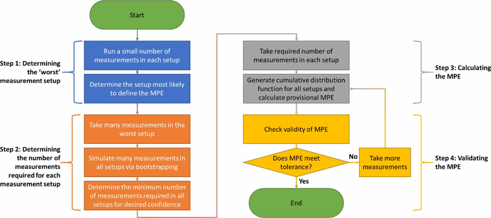
The simplest route to confidence in a determined MPE would be to take a large number of repeat measurements for all measurement setups. However, this 'brute force' method is often excessively time consuming. As such, we propose a targeted procedure for efficient data collection, supplemented by statistical resampling. This procedure follows four steps, outlined here, summarised in figure 1 and detailed throughout the following sections.
- (a)Step 1: Acquire a small number of measurements for each measurement setup and determine the setup most likely to contribute the maximum error measurement.
- (b)Step 2: Take a large number of measurements for this setup and determine the minimum number of repeat measurements required for each other measurement setup to suitably determine the MPE.
- (c)Step 3: Take the required number of repeat measurements in all remaining measurement setups.
- (d)Step 4: If there appear to be multiple setups that could contribute a maximum error measurement, consider taking a large number of measurements for those setups to reduce uncertainty in MPE determination.

Figure 1. Flowchart summarising the MPE determination method.
Download figure:
Standard image High-resolution imageIt should be noted that, while an MPE theoretically represents the upper bound of the 100% prediction interval for the measurement error, it will rarely actually represent the 100% prediction interval in practice. If we assume the value taken by any one measurement acquired using some instrument will lie along some generalised extreme value distribution bounded by the spatial frequency response of the instrument, we must also assume that it is statistically possible to acquire a value for any measurement made by the instrument anywhere between the bounds of the distribution. In practice, this means that any MPE representing the 100% prediction interval must be equal to the largest distance that instrument is capable of measuring, irrespective of how unlikely many measurements are to take this value. Such an MPE would be of little value to either consumers or instrument manufacturers, so, in practice, the MPE must represent the upper bound of some other prediction interval. For this e.g. we have set the coverage level of that interval at 99.9%, though other (high) coverage levels could be used.
3.1. Step 1—determining the 'worst' measurement setup
First, we determine which measurement setups are most likely to provide the largest error (and hence dominate the eventual MPE value). Performing this step allows a drastic reduction in the required number of measurements, made possible by the fact that an MPE is, by definition, an extreme measurement error, which allows us to discard cases where the expected error is small. To make this decision, we must acquire a small number of repeat measurements in each available measurement setup for a given system. We arbitrarily suggest that 50 or more repeat measurements are made in each setup, depending on the available time, and expected inter-measurement variation. Fifty measurements are suggested to present a reasonable distribution in many cases, but this number may differ in certain scenarios (see figure 2 as an example). The important consideration in choosing this number is that the number of measurements must be able to provide an approximate picture of the most influential measurement setup(s). To enable quantitative selection of the critical measurement setups, both the absolute mean error and the variance of each setup must be considered. Setups that have large absolute mean error and/or large variance are more likely to increase the MPE.

Figure 2. Synthetic example data for 50 initial measurement errors for ten measurement setups.
Download figure:
Standard image High-resolution imageIn figure 2, we present ten arbitrarily different, fictitious 'measurement setups', with 50 synthetic 'measurements' generated for each setup. These fictitious setups do not translate to any tangible measurement setups in some real instrument, their only real characteristics are that they differ in an arbitrarily chosen fashion from one another, in terms of the 'measurements' they provide. In the fabricated example, we have deliberately produced data that exhibits an approximately normal distribution for each setup. As can be seen in the figure, some setups result in greater deviations from nominal than others. The synthetic data are simulated by, first, randomly generating means and standard deviations for ten normal distributions with a set of means between −1 and 1 and standard deviations between 0 and 0.3. Some randomness is then added on top for the standard deviations (multiplying the standard deviation by a random floating-point number between 0.5 and 1.5) to blur the hard cut-offs set for the different parameter limits, and the greatest maximal endpoint of the symmetric 99.9% CIs centred on the mean of each of the ten distributions is taken as the MPE. The distributions are then modified so that the MPE is 1 arbitrary unit, by multiplying the mean of each distribution by a normalisation factor equal to 1 divided by the calculated MPE. These final distributions are then, finally, randomly sampled to create the final ten sets of synthetic data with an analytically correct MPE of 1 arbitrary unit.
While in this example, the implication from a visual assessment of the data is that measurement setup 3 is dominant, through examination of figure 2 alone we cannot quantify (or, consequently, automatically determine) which setup is most likely to dominate the MPE determination process. As such, each measurement setup dataset was quantified using a metric, calculated as the endpoint of the 99.9% CI (using t-distributions with 49 degrees of freedom) and taking the maximal endpoint of each synthetic dataset. To calculate these values, a distribution is fitted to each dataset and the CI of that distribution calculated. We then record the absolute values of the endpoints of the CI to determine the dominant measurement setup. The distribution used is chosen based on a reasonable assumption about the distribution of the data. As the synthetic data in this example were deliberately approximately normally distributed, a normal distribution is fitted. The endpoints of the 99.9% CI are then calculated for these normal distributions as:

where  is the estimated mean,
  is the estimated standard deviation and
  is the 99.95% quantile of the normal distribution (see figure 3 for a plot of these values; here
  ). As can be seen in figure 3, the maximal (in absolute terms) endpoint of the 99.9% CI for measurement setup 3 is the greatest, so we assume that this setup is the most likely to dominate the MPE determination process and pass this setup into step 2.

Figure 3. Maximal endpoint of the 99.9% CIs for each measurement setup presented in figure 2.
Download figure:
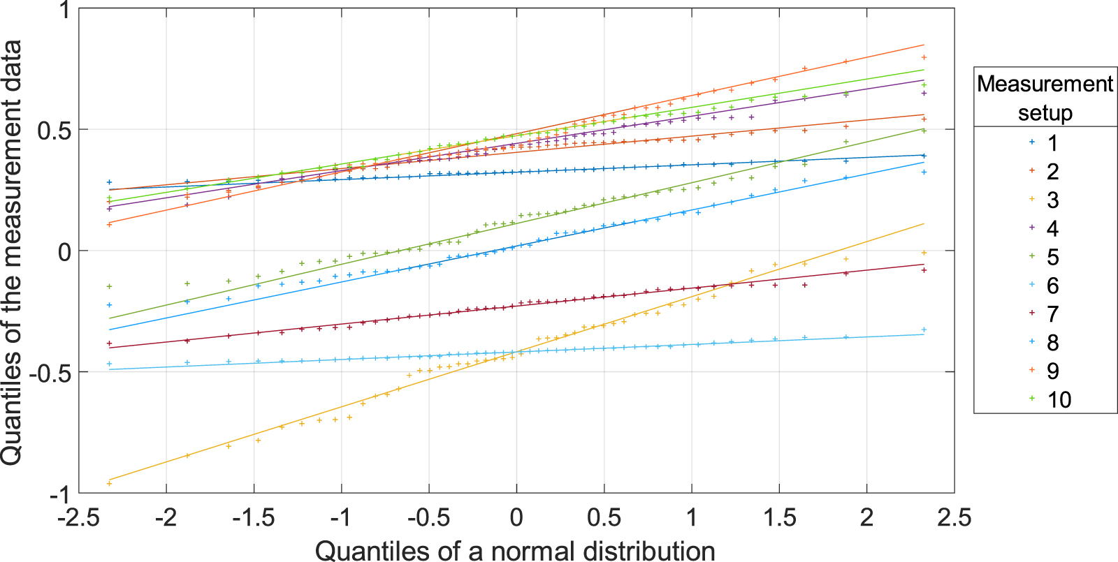
Standard image High-resolution imageBefore moving to step 2, the success of the distribution fitting should also be evaluated, using, for e.g. Q–Q plots. In this synthetic example, the Q–Q plots presented in figure 4 confirm that a normal distribution is appropriate for describing each of the ten samples of 50 observations, as an approximate linear relationship between the quantiles of a normal distribution and the quantiles of the data is present in each measurement setup. For brevity, here, a simple visual check is used but an automatic check could also be carried out using a statistical test (e.g. the Kolmogorov–Smirnov test [18] or the Anderson–Darling test [19]). Visual checks and automatic checks complement each other: automatic checks return a single number that is easy to interpret, while Q–Q plots give more extensive information about the distribution and will indicate where (if any) departures from the model distribution occurs.

Figure 4. Q–Q plots of the 1st 50 synthetic measurements for a normal distribution fitted to each dataset.
Download figure:
Standard image High-resolution image3.2. Step 2—determining the number of measurements required for each measurement setup
Once the measurement setup most likely to define the MPE value is determined, a large number of repeat measurements should be taken for the chosen measurement setup (we arbitrarily suggest at least 1000 measurements where a level of 99.9% is required). Thousand measurements are suggested to present a reasonable distribution in many cases, but this number may differ in certain scenarios. Ultimately, this number should be as large as the user is capable of measuring within a reasonable timeframe. The larger the number of repeat measurements made at this stage, the better—for the synthetic example, we have fabricated a sample of 10 000 measurements (see figure 5(a)).

Figure 5. Determination of the of repeat measurements required for each other measurement setup using measurement setup 3: (a) deviation from nominal value for 10 000 measurements; (b) normal distribution fitted to deviations; (c) PDF of the maximal endpoint of the 99.9% CI for each bootstrap, with a normal distribution fitted to infer the maximal endpoint of the 99.9% CI of the population; and (d) convergence of the setup-specific MPE to the estimated maximal endpoint of the 99.9% CI.
Download figure:
Standard image High-resolution imageWe then use the measurement data to calculate the minimum number of repeat measurements required for other measurement setups. To this end, we fit a normal distribution to the data (figure 5(b)) and calculate the maximal endpoint of the 99.9% CI for this sample, which takes the value of −1.0010 arbitrary units (represented by the dashed vertical line in figure 5(b)). In this instance, the value is negative because setup 3 generally produced negative deviations from the nominal, but a modulus of this value can be taken as the maximum deviation from nominal.
Next, we use bootstrapping to simulate 10 000 bootstrap samples (each containing 10 000 measurements) and calculate the maximal endpoint of the 99.9% CI for each of the bootstrap samples. Ultimately, this number should be as large as the user is capable of simulating in a reasonable timeframe. These 10 000 values for the maximal endpoint of the 99.9% CI of each bootstrap sample are then plotted on a 2nd frequency plot (figure 5(c)). To facilitate the next step in this process, we fit a normal distribution to this plot to create a probability density function (PDF). We then calculate the mean of the PDF, which approximates the mean of the sample of potential endpoints of 99.9% CIs. The mean value in this case was −1.0009 arbitrary units (represented by the dashed vertical line in the centre of figure 5(c)).
With this information, as we are interested in defining an MPE, we can construct a confidence interval for the endpoint of the 99.9% CI at a given confidence level,  %, and think of the appropriate endpoint of this confidence interval as an MPE for this particular setup. The point is to ensure that the provided value is almost always an over-estimate of the 'true' maximal endpoint of the 99.9% CI. A conservatively appropriate choice is p = 0.1%, which ensures that a measurement instrument would fail a performance verification test against this MPE 0.1% of the time, though other confidence levels could be chosen. The value taken by the setup-specific MPE in this example is −1.0155 arbitrary units (represented by the dashed vertical line to the left side of figure 5(c)).
The value taken by the setup-specific MPE depends upon the number of measurements made—with an infinite number of measurements, the value will equal the true 99.9% quantile, with the value diverging further from the true value the smaller the number of measurements. To determine a reasonable minimum number of measurements required in other setups, we propose the following procedure.
- (a)Record the estimated mean of the distribution of endpoints of the 99.9% CI (i.e. the dashed vertical line in the centre of figure 5(c), which here is −1.0008 arbitrary units).
- (b)For a given fictitious sample size, m, calculate the setup-specific MPE based on bootstrap samples of m measurements (for m = 10 000, this would be the dashed vertical line to the left side of figure 5(c)).
- (c)Plot the deviation of the setup-specific MPE in (b) against the estimated mean in (a) as a function of m.
This deviation gives us an idea of the uncertainty in the measurement of the MPE, which should be suitably small to ensure that the calculation of the MPE is reliable. In (a), the mean of the distribution acts as a (hopefully good) estimate of the true value of the endpoint of the 99.9% CI, which is, of course, unknown.
In figure 5(d), the deviation from the estimated maximal endpoint of the 99.9% CI rapidly reduces as the number of measurements increases. Increasing the number of repeat measurements from the 10 000 measured to 15 000 via bootstrapping does not greatly improve the estimator's convergence or the expected standard errors. Fifteen thousand bootstrap samples are used here to simulate the effects of performing significantly more measurements than initially acquired—we (arbitrarily) recommend the number used here should be 150% of the number of measurements acquired in the initial run. The deviation against the number of measurements is presented in figure 5(d) as a mean and upper and lower bound, computed by repeating this step three times, generating new sets of 10 000 bootstrap samples for each number of measurements each time. While we have presented this information in figure 5(d) below, the upper and lower bound lines are almost indiscernible from the mean line because of small deviations between repeat experiments. In figure 5(d), a modulus of the calculated population 99.9% CI is presented to provide a positive maximum deviation from the nominal value.
When calculating the convergence plot (figure 5(d)), continuous sub-sections of size m of the data collected for that measurement setup are first randomly chosen. Bootstrap samples are then created from these sub-sections, also of size m and the setup-specific MPE is calculated for each m from the bootstraps. The deviation of these setup-specific MPEs from the estimated mean of the distribution of endpoints of the 99.9% CI is then plotted against m. This whole process is then repeated three times, and a different continuous sub-section is chosen for each repeat of the process. In the figure, the dashed lines show the envelope of the highest and lowest calculated MPE against the number of measurements, across the number of repeats employed (three, here). In this implementation, if the number of measurements multiplied by the number of convergence test repeats is less than the number of available measurements, the raw data is separated into the same number of sections as there are repeats, and each simulated data collection run is randomly positioned within that section. If the number of measurements multiplied by the number of convergence test repeats is more than the number of available measurements, the beginning of the simulated data collection runs is overlapped with a random offset, without overhanging the end of data collection (as wraparound sampling is not ideal because of the potential presence of drift [8]). If the simulated number of measurements is more than the number of available measurements (so wraparound sampling is unavoidable), the data are tiled to the extent specified by the oversampling ratio and a random starting point offset is again used. This overall procedure is used to limit the influence of small-scale irregularities when the number of measurements is small.
The data presented in figure 5(d) is finally used to determine the number of measurements required for other measurement setups to determine the overall MPE, by applying a threshold to the convergence. The value at which this threshold is applied is ultimately determined by the user; here we have arbitrarily set the value to 5% of the calculated setup-specific MPE (the central dashed line in figure 5(c)), which in this synthetic example is 0.0508 arbitrary units (represented by the dashed horizontal line in figure 5(d)). By examining the intersection between the upper bound of the convergence line and the threshold and rounding up to the nearest integer, in this synthetic example we determine that the required number of measurements is 2147.
3.3. Step 3—calculating the MPE
Once the minimum number of measurements per setup has been determined, that number of measurements is made in all remaining measurement setups (nine setups, in this example). Bootstrapping of all the repeat measurements from these setups is then carried out, creating a very large number of bootstrap samples (100 000 bootstrap samples, in this example). One lakh bootstrap samples are used here to simulate the effects of performing a much larger number of measurements than initially acquired—we (arbitrarily) recommend the number used here should be 1000% of the number of measurements acquired in the initial run. As in step 2, this number should be as large as the user is capable of simulating in a reasonable timeframe. These bootstrap samples contain the number of measurements equivalent to the number of measurements taken for each setup (here, 10 000 for measurement setup 3 and 2147 for all other setups). Frequency plots are generated for each setup (similar to that shown in figure 5(c)) and a normal distribution is fitted to each of these plots). These normal distributions are shown plotted on a single graph in figure 6(a). To generate figure 6(b), we first take the cumulative distribution function (CDF) related to each of the individual frequency functions, and then take the product of all these functions to create the overall CDF presented in the figure. Mathematically, this step corresponds to estimating the CDF of the maximum deviation across the ten independent setups. In this overall CDF, the 99.9% quantile (i.e. corresponding in some sense to a one-sided tolerance interval) then represents the calculated MPE. The calculated value of the MPE is finally 1.0152 arbitrary units (represented by the dashed vertical line to the right side of figure 6(b)).

Figure 6. First-pass calculation of the MPE: top; distribution of the maximal endpoint of the 99.9% CIs from bootstrapped data for each measurement setup; and bottom; product CDF, with the 99.9% quantile highlighted.
Download figure:
Standard image High-resolution image3.4. Step 4—validating the calculated MPE
Having collected and analysed all the required data, it is important to evaluate the quality of the calculated MPE. In this example, measurement setup 3 is clearly the most dominant contributor to increasing the MPE. However, cases are likely to exist in practice where more than one measurement setup will have similar contributions to increasing the MPE, or where the dominant setup is not sufficiently sampled. If there are multiple measurement setups that similarly dominate the MPE determination, or a lack of measurements in the dominant measurement setup, it is prudent to collect further repeat measurements, to reduce overestimation of the MPE due to uncertainty caused by insufficient sampling.
To determine whether the calculated MPE is 'good enough', some user-defined criteria must be employed. In this case, the dominant measurement setup is chosen after the initial set of measurements, steps 1–3 are followed and the MPE recalculated. Then, the areas under the frequency plots presented in figure 6 are examined, and the measurement setup with the greatest area beyond the calculated MPE is chosen. If the 90% interquantile range of the product CDF (given by the curve in figure 6(b)) is greater than some predefined tolerance (here, arbitrarily, 5% of the calculated MPE), then further measurements should be acquired in the chosen measurement setup, the assumption being that the uncertainty on the calculation of the MPE is still too high for this estimate to be reliable. We suggest that this number of measurements is equal to the difference between the large number of measurements used at the beginning of step 2 and the number of measurements already acquired (unless this value is zero, in which case, we suggest taking an extra number of measurements as in the beginning of step 2, i.e. to take 20 000 observations in total if the original number was 10 000).
This process should be iterated until the gap is smaller than the predefined tolerance. In this synthetic example, this test was passed in the 1st MPE calculation and no further measurement was required. As such, the final efficient determined MPE for this synthetic example is 1.0152 arbitrary units, as calculated in step 3. This value is, as expected, over-estimated with respect to the analytically true MPE of 1 arbitrary unit but is, in fact, within 1.6% of that value.
In this example, the method has been used to define an MPE (i.e. corresponding to a prediction interval) that is valid for 99.9% of measurements (i.e. one random failure is to be expected per 1000 measurements). Using the method described here, we can provide a confidence level for that prediction interval, which we have also set at 99.9%. In summary, we are (approximately, and subject to checks on the underlying distribution of measurement deviations) 99.9% certain that this method produces an MPE value that, when tested, will result in one performance verification failure in every 1000 tests, solely as a result of random chance. This statement represents a tolerance interval for this method.
3.5. Synthetic validation
To demonstrate the validity of the method, we repeated the whole process 1000 times, determining 1000 separate MPEs, using an entirely new set of synthetic data each time. Further repetitions are possible, but running the whole experiment is computationally expensive.
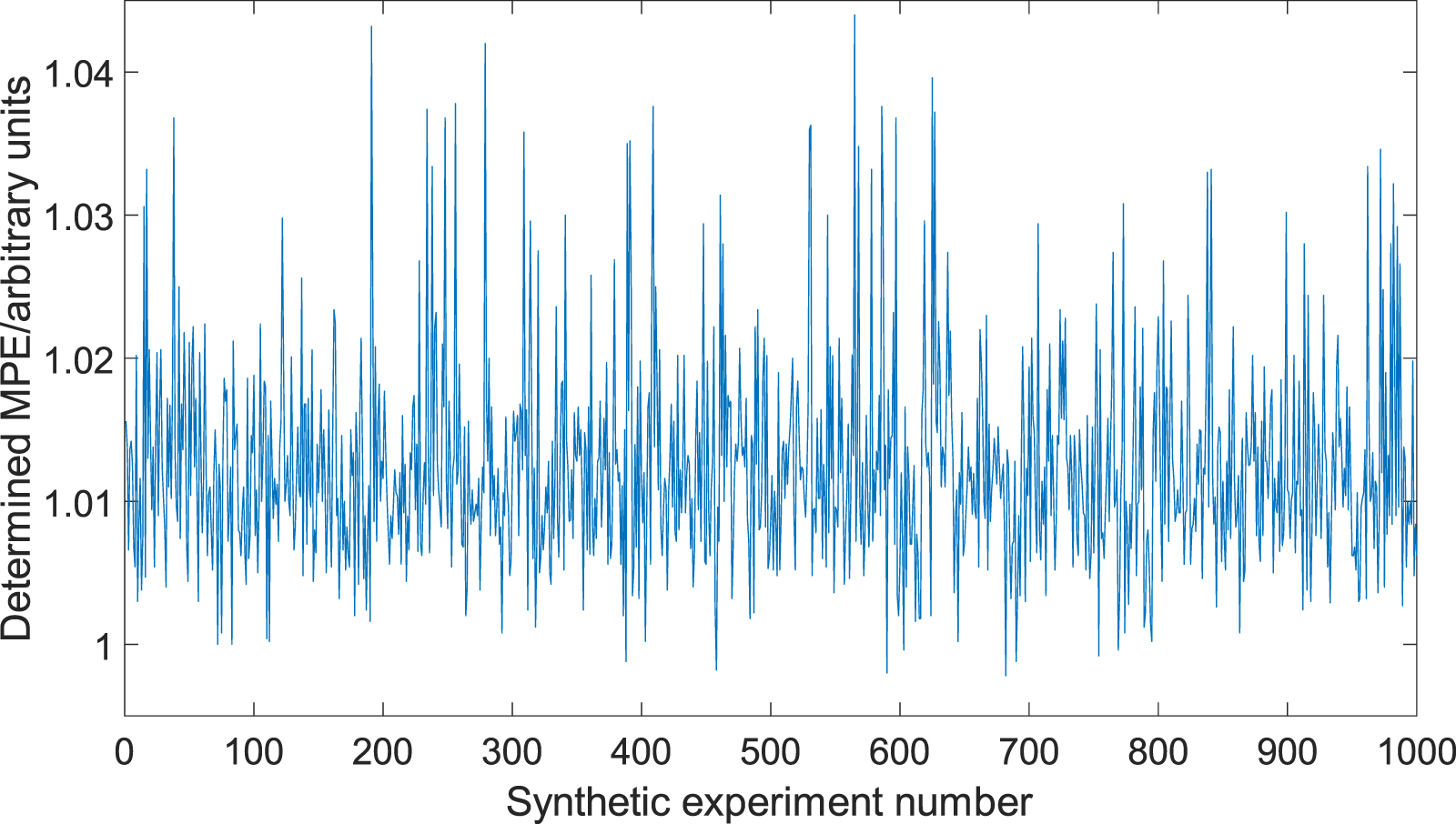
As discussed in the introduction to section 3, the analytically true MPE for this synthetic example is 1 arbitrary unit. As can be seen in figure 7, over 1000 repeats of the whole process, the method resulted in an underestimation of the MPE eight times (underestimated, on average, by 0.13% and at most by 0.22% of the true value). The method resulted in no large overestimations of the MPE (>10% of the true value). The mean and standard deviation of the determined MPE over 1000 repeats of the whole process were 1.0124 and 0.0070 arbitrary units, respectively, equivalent to an error of 1.24% ± 2.30% (at 99.9% confidence, using a t-distribution with 999 degrees of freedom equivalent in practice to a normal distribution).
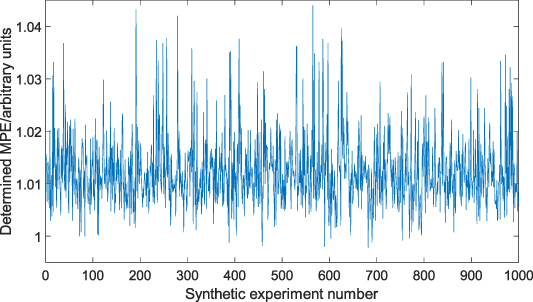
Figure 7. The efficient determined MPE over 1000 repeat experiments, where the true value is 1. Values greater than one represent the efficient MPE being larger than the true MPE (i.e. overestimation), with values less than one representing the converse.
Download figure:
Standard image High-resolution image4. Experimental validation of the method
We present the results of a practical implementation of the method reported in this paper, using a commercial fringe projection system. The system used here is tested against an example MPE discussed in the current draft of ISO 10360-13 [2, 7], particularly the 'probing form dispersion error' for a single-view sphere measurement (i.e. the thickness of a spherical shell which encompasses measured data acquired using a single fringe projection measurement). In this case, 100% of measured points were used to calculate the probing form dispersion error. Using the symbol convention presented throughout the ISO 10360 series, this MPE is denoted PForm.Sph.All:SMV:SV:O3D,MPE. The 100% probing form dispersion error was chosen for its relative simplicity as a real-world test case. In this example, the distribution of errors is expected to be a generalised extreme value distribution, which can have significant tails and is, therefore, likely to be more challenging to accurately fit distributions to than a normal distribution [7].
It should be noted that, as ISO 10360-13 [7] has not yet been published, existing systems cannot yet be expected to conform to the standard and so performance verification results may differ from those expected by the instrument manufacturer. Particularly, the MPE generated using our method may not necessarily marry up to any MPE(s) that have been published for the test system. As such, details regarding the specific test system used in this work have been withheld, to prevent misrepresentation of a commercial measurement system.
4.1. Measurement procedure
A calibrated sphere was measured in eight different measurement setups (defined in ISO 10360-13, where they are referred to as 'positions' [2, 7]) using the fringe projection system. These positions are obtained by placing the sphere at different locations within the instrument measurement volume. Under the assumption that the instrument measurement volume is a cube, that cube is subdivided into eight equally sized cubes and the sphere is place in each of these cubes in sequence. The positions are numbered such that the four cubes closest to the instrument are 1–4 and those furthest away are 5–8. At each level, the lowest numbered cube is in the top left of the field of view, as seen by the instrument, with increasing numbers progressing anticlockwise from the top left (see [2] for a visualisation of this setup). Each measurement setup was achieved by either moving the measurement system, the measured artefact or a combination of both actions. In each case, the sphere was positioned close to the edge of the measurement volume. For reasons of practicality of data collection, repeat measurements were made in each measurement setup, before moving the physical measurement setup into the next pose. This method reduces the number of measurement setup transitions, which reduces the time required for measurement and breaks any correlation between measurement setups. It should be noted that if, in some practical application, a strong correlation between measurements is introduced by the ordering of measurements, the measurement procedure should be modified to reduce such effects. Although theoretically possible, it is beyond the scope of this paper to account for such temporal correlations when calculating an MPE.
The sphere measured during this work adhered to the specification presented in ISO 10360-13 and had minimum and maximum deviations from a Gaussian substitute sphere of—(0.88 ± 1.8) µm and (1.07 ± 1.8) µm, respectively (expanded uncertainty presented at k = 1.96). The sphere was calibrated using a CMM by an ISO 17025-accredited 3rd party [20].
4.2. Step 1—determining the 'worst' measurement setup
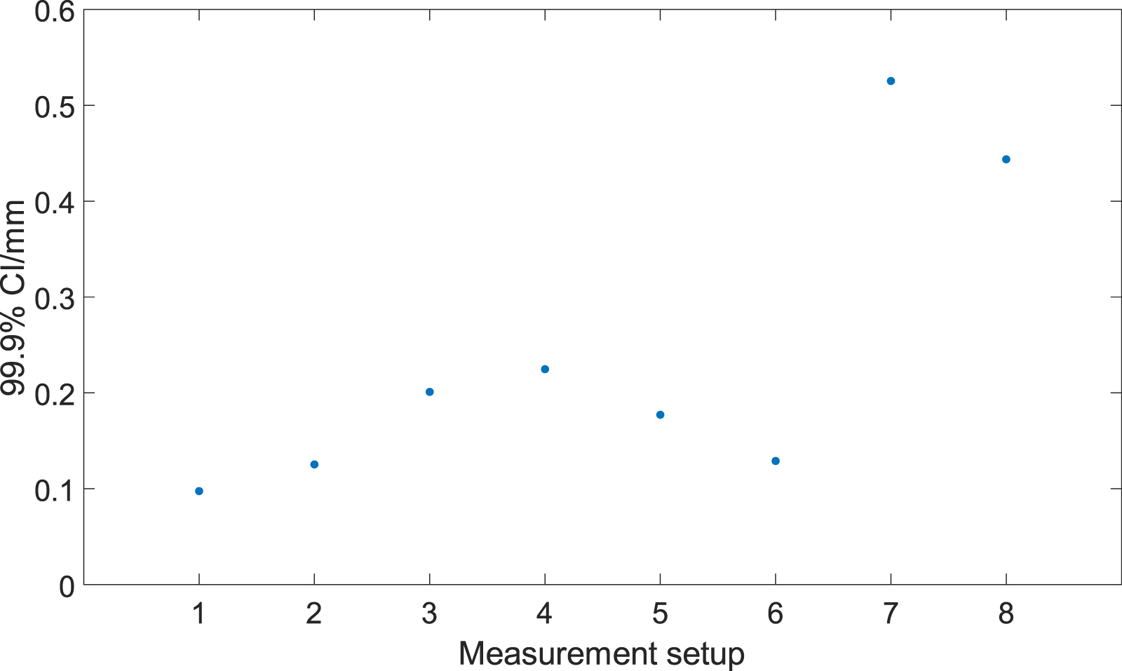
To begin, 50 measurements were acquired of the calibrated sphere in each of the eight measurement setups. In each case, a minimum-zone spherical shell encompassing 100% of the data points was fitted to the acquired point cloud data and the probing form dispersion error was calculated as the thickness of these shells. Data acquisition was performed using the manufacturer's proprietary software, while sphere fitting and calculation of the probing form dispersion error was performed in Polyworks 2019 [21]. The probing form error calculated from each measurement is presented in figure 8. The plot of the maximal endpoint of the 99.9% CIs for each measurement setup presented in figure 9 suggests that measurement setup 7 represents the worst measurement. The Q–Q plots presented in figure 10 confirm that the assumption that measurements follow a generalised extreme value distribution is overall reasonable in this case, up to small-sample variability in setups 4 and 7. The specific type (I–III) of generalised extreme value distribution is automatically determined according to best fit using maximum likelihood estimation, on a dataset-by-dataset basis.

Figure 8. Measured data for 50 initial measurement errors for eight measurement setups.
Download figure:
Standard image High-resolution image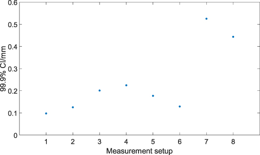
Figure 9. Maximal endpoint of the 99.9% CIs for each measurement setup presented in figure 8.
Download figure:
Standard image High-resolution image
Figure 10. Q–Q plots of the 1st 50 measurements for a generalised extreme value distribution fitted to each dataset.
Download figure:
Standard image High-resolution image4.3. Step 2—determining the number of measurements required for each measurement setup
With measurement setup 7 chosen as the measurement setup most likely to define the MPE, 1000 measurements were acquired in this setup, to determine the minimum number of measurements required in each of the other measurement setups. This information is presented in figure 11. By fitting a generalised extreme value distribution to the data (figure 11(b)), we calculate the maximal endpoint of the 99.9% CI for this sample, which in this example takes the value of 0.496 mm (represented by the dashed vertical line in figure 11(b)).

Figure 11. Determination of the of repeat measurements required for each other measurement setup using measurement setup 7: (a) deviation from nominal value for 1000 measurements; (b) generalised extreme value distribution fitted to deviations; (c) PDF of the maximal endpoint of the 99.9% CI for each bootstrap, with a generalised extreme value distribution fitted to infer the maximal endpoint of the 99.9% CI of the population; and (d) convergence of the setup-specific MPE to the estimated maximal endpoint of the 99.9% CI.
Download figure:
Standard image High-resolution imageUsing bootstrapping to simulate 10 000 samples, we then calculate the maximal endpoint of the 99.9% CI for each of the bootstrap samples, plot these as a frequency plot (figure 11(c)) and fit a generalised extreme value distribution to this plot to create a PDF. The mean and upper value of the 99.9% CI of the PDF were 0.496 mm (represented by the dashed vertical line in the centre of figure 11(c)) and 0.523 mm (represented by the dashed vertical line to the right side of figure 11(c)), respectively. This latter value is the estimation of the setup-specific MPE for setup 7.
The convergence threshold was taken as 5% of the maximal endpoint of the 99.9% CI (here, 0.026 mm) and the intersection between the upper bound of the convergence line and this threshold determined using the plot in figure 11(d). In this example, the convergence line crosses the threshold more than once, so we take the larger of these intersections as the required number of measurements, which in this case is 512. Here, it is important to note the slightly erratic behaviour of the three curves for a number of measurements lower than 250, due to small-sample variability; this behaviour is another reason why taking a relatively large number of measurements is important.
We can also use this step to perform further validation of the decisions made as part of the method. Particularly, figure 11(b) shows that the distribution of deviations from the nominal in measurement setup 7 is reasonably well approximated by a generalised extreme value distribution. Also, the convergence to the estimated population mean with increasing bootstrap size (shown in figure 11(d)) suggests that the 1000 measurements performed were sufficiently numerous to accurately estimate the maximal endpoint of the 99.9% CI. This conclusion is supported by two aspects of the figure 11(d), particularly: above around 500 measurements, the difference between the upper and lower bound of the convergence plot is small compared to the measured deviations; and there seems to be no significant benefit to acquiring more than around 700 measurements.
4.4. Step 3—calculating the MPE
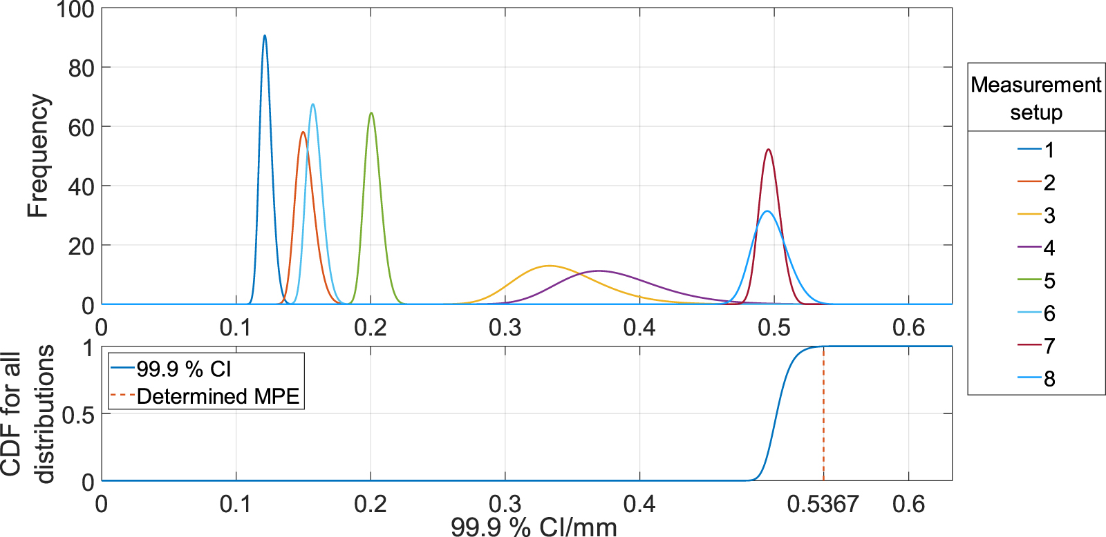
Five hundred and twelve measurements were then made in all remaining measurement setups. Bootstrapping of all the repeat measurements from these setups is then carried out, creating a very large number of bootstrap samples (100 000 bootstrap samples, in this example). These bootstrap samples contain the number of measurements equivalent to the number of measurements taken for each setup (here, 1000 for measurement setup 7 and 512 for all other setups). Frequency plots were generated for each setup and a generalised extreme value distribution fitted to each of these plots (see figure 12(a)). Figure 12(b) is then the CDF created from taking the product of all of the pertaining CDFs, with the calculated value of the MPE, determined as the 99.9% quantile of this distribution, being 0.537 mm (represented by the dashed vertical line to the right side of figure 12(b)).

Figure 12. First-pass calculation of the MPE: top; distribution of the maximal endpoint of the 99.9% CIs from bootstrapped data for each measurement setup and bottom; product CDF, with the 99.9% quantile highlighted.
Download figure:
Standard image High-resolution image4.5. Step 4—validating the calculated MPE
In this example, measurement setup 7 was initially chosen as the most dominant contributor to increasing the MPE. On examination of the area under the frequency plots presented in figure 12, measurement setup 8 was found to have the greatest area beyond the calculated MPE and the width of the tolerance interval (i.e. the 99.9% quantile of the curve in figure 12(b)) was greater than the predefined tolerance (here, 5% of the calculated MPE) multiplied by the calculated MPE. As such, a further 488 (i.e. 1000 total) measurements were acquired in measurement setup 8. A recalculation of the MPE, following further measurements made in measurement setup 8, is presented in figure 13, where the calculated value of the MPE is 0.528 mm (represented by the dashed vertical line to the right side of figure 13(b)).

Figure 13. Determination of a final MPE following additional measurement in measurement setup 8: top; distribution of the maximal endpoint of the 99.9% CIs from bootstrapped data for each measurement setup and bottom; product CDF, with the 99.9% quantile highlighted.
Download figure:
Standard image High-resolution imageFurther examination of the area under the frequency plots for this new MPE showed that measurement setup 8 retained the greatest area beyond the calculated MPE, but that the width of the tolerance interval was now smaller than the 5% predefined tolerance multiplied by the calculated MPE. As such, no further measurements were deemed necessary and the efficient determined value of the MPE is 0.528 mm, as calculated above. This final MPE was calculated with 512 measurements acquired in measurement setups 1–6 and 1000 measurements acquired in measurement setups 7 and 8.
To finally demonstrate the validity of this method, we acquired 1000 measurements for each of the other six measurement positions and repeated step 3 of the analysis, to provide a brute-force approach to MPE determination. The outcome of this validation is presented in figure 14, where the brute-force value taken by the MPE is 0.526 mm (represented by the dashed vertical line to the right side of figure 14(b)). As shown in figure 14, measurements setups 7 and 8 remained dominant. The efficiently determined MPE is over-estimated with respect to the MPE determined using a significantly larger amount of data but is within 0.3% of that value.

Figure 14. Brute-force validation of the data-efficient determined MPE, using 1000 measurements for each measurement setup: top; distribution of the maximal endpoint of the 99.9% CIs from bootstrapped data for each measurement setup and bottom; product CDF, with the 99.9% quantile highlighted.
Download figure:
Standard image High-resolution image
5. Discussion
The procedure described here provides a statistical method for determining an MPE that requires few user-defined parameters and a minimum number of repeat measurements. The method has been illustrated using both synthetic and experimental data. Here, we discuss the efficiency of the method with respect to a brute-force method of MPE determination, as well as potential drawbacks (such as user-defined algorithm control parameters) and improvements to the method presented.
The first question to ask, with respect to the example experimental MPE produced using this method, is how the value compares with the equivalent MPE supplied by the manufacturer. However, as discussed previously, no comparisons can be made between the value calculated in this example and the manufacturer supplied MPE, as the manufacturer does not yet apply an ISO 10360-13 performance verification procedure (because the standard is still in a draft form). However, comparison between the efficient MPE and the MPE determined using a large number of measurements can be used as an indicator of effects of using a relatively small sample size. The efficient MPE was larger by 0.3%.
Beyond comparison between efficient and brute-force MPE values, the next question to ask is how efficient the method is with regards to a brute-force method of MPE determination. To demonstrate the efficiency of the MPE determination method (i.e. the time savings provided by this method relative to a brute-force method involving many measurements in each possible setup), we present the measurement and computation time required for each of the steps of the procedure in table 1. While the measurement time heavily dominates the total time taken in both the efficient and brute-force cases, we have noted the general specifications of the computer used for computation here, alongside computation times. A desktop computer with a four core, 3.4 GHz CPU and 32 GB RAM was used for the analysis, with parallelisation used for the bootstrapping process. The time required to generate an MPE by collecting a large number of measurements (1000 per measurement setups) was 60.9 h, including computation time, but by employing the efficient method, the total time to calculate an MPE was reduced to 37.3 h (including computation time).
Table 1. Measurement and computation time for each step of the method.
| Process step | Efficient measurement time/hours | Brute force measurement time/hours | Efficient computation time/hours | Brute force computation time/hours |
|---|---|---|---|---|
| Step 1 | 3.0 | 0 | 0.0 | 0.0 |
| Step 2 | 5.6 | 0 | 1.6 | 0.0 |
| Step 3 | 25.1 | 60.3 | 0.2 | 0.6 |
| Step 4 | 2.6 | 0 | 0.1 | 0.0 |
| Total | 36.4 | 60.3 | 1.9 | 0.6 |
Whilst the experimental validation of the method followed a specific performance verification process, the estimation approach presented is general and can be used to determine a type A MPE (i.e. by the statistical analysis of a series of observations [9]) for any scenario. If a new measurement routine and environment was developed for an existing measurement system, for e.g. the efficient collection of data would allow for robust error analyses for arbitrary measurement procedures and environments. Although the experimental data was collected manually, automation systems, such as robot arms and rotation stages would significantly reduce the need for required operator intervention. Due to the minimal requirement for operator decision making during the analysis process, it would be feasible for the MPE determination process to be automated. Automation would reduce the additional resource needed for MPE determination to just the measurement time required to collect sufficient data, which could potentially be carried out during planned idle periods. Whilst the bootstrapping required by the analysis is somewhat computationally intensive, the experimental determination procedure was performed using a relatively basic desktop computer in approximately 2 h, using data that required approximately 36.4 h to collect. Graphical processing units could be used to accelerate the bootstrapping process and significantly reduce the time taken to complete the data analysis [22], but we expect that the time taken for data collection will exceed the required analysis time in the majority of applications.
It is clear that there is also potential for interrogating measurement data to carry out type B uncertainty analysis of the measurement system (i.e. by means other than the statistical analysis of series of observations [9]), for e.g. by examining the large number of repeat measurements alongside environmental monitoring, to evaluate the sensitivity of the measurement systems to variables such as temperature and humidity. This is a caveat to the proposed method: if the measurement environment changes significantly from that present during MPE determination (such as a temperature change in the measurement volume, beyond a defined tolerance), then the determined MPE is invalid (though this issue is true of any type A MPE determination). A full type B assessment is a more complex and resource intensive process that, as far as we are aware, has not yet been reported for a fringe projection system in literature [23]. Such investigations are beyond the scope of this paper but present an interesting avenue for future research.
Additionally, while the majority of the steps in this method are automated, there are eight parameters that control the outcome of the analysis, meaning that the determined MPE remains somewhat user-defined. Certain checks should ideally be implemented regarding these user-defined parameters to ensure a reasonably defined MPE. These parameters, and appropriate checks, are as follows.
Two parameters are fully user-defined without checks. These parameters should be fixed at the beginning of the MPE determination process, to prevent the user artificially lowering the calculated MPE post-analysis.
- Desired CI (i.e. the probability that a performance verification test will not be failed due to random chance)—defined by the user for use throughout the process.
- Desired confidence level (i.e. the confidence held in the desired CI)—defined by the user for use throughout the process.
Four parameters are user-defined but checked by both the Q–Q plots and the convergence test in step 2.
- Expected statistical distribution of the measured data—checked with Q–Q plots.
- Initial sample size—checked with Q–Q plots.
- Number of repeats used for large datasets—checked with convergence plot (i.e. figures 4(d) and 10(d)).
- Number of bootstraps used—tested with convergence plot.
Q–Q plots illustrate the variation in fitting success at the tails of the distribution. Decisions about which distributions to use for fitting require knowledge of the measurement and should be made by an experienced user of the measurement system, although they will typically be chosen among a small range of well-known probability distributions, such as the normal and generalised extreme value distributions. The other two parameters are checked by the convergence test in step 2. Particularly, if increasing the sample size beyond the initial user-defined number of repeat measurements is shown by the test to be beneficial, the user is notified of the need to acquire additional measurements. Additionally, the bootstrap sample size determination provides the repeatability of the bootstrapped CI estimates, where, if the number of bootstraps is too low, then the CI estimate will be unstable.
Two final parameters affect efficiency and are not inherently checked by the process. This uncertainty is accounted for in the calculated MPE, so the user can choose their desired compromise between measurement efficiency and MPE uncertainty.
- Number of repeats used to create the convergence plot—minimally affects the accuracy of the determined MPE but increasing the number of repetitions is computationally more expensive.
- Remeasuring criteria—affects efficiency, but the trade-off between performance and measurement efficiency is a user choice.
It is also useful to note areas where the method may be improved. The most obvious deficiency in the method is during step 4, in the case where the tolerance interval is greater than the predefined tolerance multiplied by the currently calculated MPE and further measurement in one or more measurement setups is deemed to be required. In this instance, the ideal version of the method would include a prediction for the number of additional measurements required in each measurement setup, to ensure that when recalculated, the tolerance interval is smaller than the predefined tolerance multiplied by the currently calculated MPE. Such a prediction is complex, however, due to noise in the measurement data, so some checking and additional further measurement would likely be required even if this prediction were made. Here, to reduce the number of user interventions in the process, we have recommended that the user acquire another large set of measurements, under the assumption that doing so will often provide enough data if the number of measurements for the setup initially thought to be most influential was large enough. However, a prediction of the minimum number of additional measurements may further reduce the total time for the MPE determination process. Such a reduction would be relatively small and designing this prediction algorithm would be complex. As such, this exercise is beyond the scope of this work, but represents an interesting avenue for future refinement of this method.
Additionally, we should note that throughout this work, bootstrap CI estimation has been performed without using a bias correction (despite being commonly employed). This approach has potential ramifications to the analytical accuracy of the method. However, bias correction is generally used when there is a significant skew in the data, which is not seen in the data we acquired throughout this work. When designing the implementation of the method in Matlab, the default distribution fitting function occasionally failed to fit an appropriate distribution to the synthetic data used to test the algorithm. As such, some small modifications were made to the fitting algorithm to cope with this issue, and CIs were then computed on the fitted distributions. This version of the CI computation algorithm did not include a bias correction, but as the skew of our data was small in both the synthetic and real cases, no further modification of the algorithm was deemed to be necessary. Research on this topic (e.g. see [24]) also notes that the greatest risk of not using bias correction is under estimation of the CI, which we have shown does not happen in 99.2% of synthetic cases when our method is employed. Of course, there is scope for incorporating a bias correction into the method in the future.
6. Conclusion
In this work, we have demonstrated a statistical method of determining MPEs within the ISO 10360 framework [1], using the minimum number of measurements possible to determine a value that fits within a user-defined specification. In addition to the statistical foundation to the determined MPE, the method is efficient in both time and data volume, compared with a brute-force MPE determination method involving the acquisition of an arbitrarily large volume of data. Through the application of 1000 separate synthetic experiments and a real test case, we have shown the method to be reliable. A framework for associating confidence levels with MPEs has also been introduced to allow for MPEs to be specified to meet measurement requirements.
Whilst determining an MPE does not involve evaluation of measurement uncertainty and cannot be used to calibrate a measurement system, within the remit of performance verification and comparison between measurement systems, MPEs are useful tools. Specifying an MPE using solely a large volume of data without any formal statistical foundation does not provide instrument users with the confidence that is commonly desired. This method could be employed by machine manufacturers for specifying MPEs in some general cases, or directly by instrument users to specify task-specific MPEs.
Further research on this topic should examine the most efficient ways to collect and analyse large volumes of measurement data to determine MPEs, as well as theoretical investigation of the accuracy and precision of such techniques. Because of the scarcity of rigorous determinations of MPEs in the literature, we hope that the presented methodology will be considered when quoting MPEs for measurement systems in the future.
Acknowledgments
A T and R K L would like to acknowledge the European Regional Development Fund ('ARTEFACT' collaborative R&D Grant) and AddQual Ltd for supporting this work, as well as Professor Nicola Senin for fruitful discussions on the topic.
Data availability statement
The data that support the findings of this study are available upon reasonable request from the authors.