


Abstract
A weighted parameter vector χnorm based on extracellular fluid resistance in the Cole impedance model is hereby proposed in order to compensate for the volatile-distributed current. The volatile-distributed current due to variance in the unknown contact impedance in an electrical impedance tomography (EIT) sensor distorts the ideality of the frequency-dependent behavior of the object of interest, leading to inaccuracy in the reconstructed images. The sources of variance in the unknown contact impedance include the use of electrodes with inconsistent impedance values, electrochemical reaction or the improper attachment of electrodes to the object of interest. χnorm represents the current pathway lengths at zero frequency which reflects the volatile-distributed current, and it is used to determine the source of the measured impedance. The source of the unknown contact impedance can be the background object in the normal physiological condition, an inclusion object in an abnormal physiological condition or systematic error. The new reconstruction methods are derived from the frequency-difference EIT (fd-EIT) and the weighted-frequency-difference EIT (wfd-EIT) using χnorm. The new reconstruction methods are frequency-difference electrical impedance spectro-tomography (fd-EIST) and weighted-frequency-difference electrical impedance spectro-tomography (wfd-EIST). The performance of fd-EIST and wfd-EIST was evaluated by experimental and simulation studies using biomaterials with frequency measurements from f = 500 Hz to f = 100 kHz and the results were compared with those from fd-EIT and wfd-EIT. The results showed that the use of χnorm reduces the root mean square error, position error, ringing and shape deformation. It also increases the ideality of the frequency-dependent behavior, either for the inclusions or the background objects at different frequencies.
Export citation and abstract BibTeX RIS
1. Introduction
Electrical impedance tomography (EIT) is a method of physiological analysis which involves injecting a feeble alternating current into an object of interest and measuring the resultant impedance through electrodes attached to its surface [1]. EIT works based on the fact that the frequency-dependent behavior of the measured impedance differs according to the nature of that impedance. EIT enables researchers in the functional imaging field to reconstruct the distribution of the electrical properties inside the object of interest. These electrical properties include conductivity σ (S m−1) and permittivity εr (unitless); these are frequency dependent and their distribution within an object of interest reflects the physiological condition of that object. EIT has therefore been effectively used in the monitoring of pulmonary perfusion [2–4] and gastric emptying [5], in the detection of breast tumors [6, 7] and in the monitoring of brain function [8]. The success of EIT in showing the changes in the physiological condition of the object of interest is based on accurate determination of the source of the measured impedance. The source of the impedance can be the background object, which is the normal physiological condition of the body, or an inclusion object, representing an abnormal physiological condition; it can also be due to systematic error as a result of poor contact between the object of interest and the EIT machine (unknown contact impedance variance).
Inherently, the attachment of electrodes to the skin causes unknown contact impedance variance as part of a systematic error in EIT. The unknown contact impedance variance appears as a result of impedance mismatch between the electrodes, electrochemical reaction or the improper attachment of electrodes to the object of interest. Generally, unknown contact impedance variance affects the accuracy of the reconstructed image of EIT in two ways: the common-mode voltage error and the volatile-distributed current I1. While the common-mode voltage error has been overcome by using common-mode feedback in modern differential amplifier circuits [9, 10], problems regarding the volatile-distributed current I1 still remain. Ideally, the distributed current from the transmitter electrodes should have the same value in all measurements in EIT based on the current–voltage measurement system (CV system). The instability of distributed current from the transmitter or the volatile-distributed current I1 distorts the ideal frequency-dependent behavior of the inclusion and background objects in EIT, leading to image artifacts [11–15]. The volatile-distributed current I1 represents the voltage drop in the transmitter due to the existence of contact impedance [16]. However, it is difficult to control the volatile-distributed current I1 because the positions of the transmitter and the receiver electrodes change during the EIT measurement procedure.
In order to overcome this difficulty, simultaneous compensation of the unknown contact impedance variance due to the volatile-distributed current I1 is necessary at each position of the transmitter and receiver electrodes [17]. Even though some authors have proposed innovative methods to compensate for the unknown contact impedance variance, such as the uniform conducting medium method [18, 19], the compensation error method [20], the statistical estimation method [21–24], skin preparation (cleaning the skin, applying conductive gel and using bandages) [14] and covering the electrode with a resistive material [25, 26], none of these methods consider the accuracy of the frequency-dependent behavior in the reconstructed images. Therefore, simultaneous compensation of the unknown contact impedance variance due to the volatile-distributed current I1 is still a significant challenge in actual EIT applications.
The novelty of this paper is to propose a weighted parameter vector χnorm based on the Cole impedance model in order to simultaneously compensate for the unknown contact impedance variance. Frequency-difference EIT (fd-EIT) and weighted-frequency-difference (wfd-EIT) modified by integrating χnorm are called frequency-difference electrical impedance spectro-tomography (fd-EIST) and (wfd-EIST), respectively. χnorm reflects the length of the current pathway which is influenced by the volatile-distributed current. fd-EIST and wfd-EIST are investigated through experimental and numerical simulation studies by using a frequency-independent background object and frequency-dependent background object biomaterials. The reconstructed images of fd-EIT, fd-EIST, wfd-EIT and wfd-EIST are evaluated with regard to the root mean square error (RMSE), position error (PE), ringing (RNG) and shape deformation (SD) for different frequencies and the ideal frequency-dependent behavior of the inclusion and background objects. Additionally, numerical simulation is used to show the effect of unknown contact impedance variance on the impedance change and the reconstructed image.
2. Compensation of the volatile-distributed current
The conventional (fd-EIT [13] and wfd-EIT [27]) and proposed (fd-EIST and wfd-EIST) reconstruction methods are compared in terms of impedance change ΔZ for reconstruction of conductivity change Δσ as follows:


where ξ is a dimensionless weighted constant which is calculated using the standard inner product of two vectors of the impedance of the object of interest from two sequential frequencies f a and f b:
Here, Za and Zb are the impedances at two sequential frequencies f a and f b, respectively.  and
and  are the real parts of the impedance of Za and Zb, respectively.
  is the weighted parameter vector, which is dimensionless.
2.1. Frequency-difference EIST
In order to compensate for the contact impedance variance, the current pathway length De (mm) is considered by calculating the normalized extracellular fluid resistance, called  (unitless), from all the measurements m as follows:

Here, Recf (Ω) is the resistance for the measurement at zero frequency f 0, and  . The total number of measurements M = 104 with ne = 16 electrodes and m = [1, ..., M]. The value of χ could be much higher than Ra − Rb. ΔZ, which has a high range order value, makes the reconstruction more ill-posed because the EIT reconstruction method proposed in this study is for cases with a small change in conductivity. Considering the ill-conditioned Jacobian matrix, in the linear regularization of EIT the value of ΔZ should be small compared with the change in conductivity, i.e. ΔZ/Δσ ⩽ 1. In this regard, χ is normalized as we proposed without losing information about the length of the current pathway.
The approximation of equation (6) is based on properties of the Cole impedance model shown in the electrical equivalent circuit in figure 1(a) [28–30]. The equivalent electrical circuit is a model of impedance with multifrequency measurements of biological tissue composed of multicellular cells, as shown in figure 1(b). The equivalent electrical circuit shown in figure 1(a) is widely used for the interpretation of the Nyquist plot of a single curve, as shown in figure 2 for biological tissue impedance measurements which have a dispersion impedance due to the complexity of electrical properties of multicellular systems with multifrequency measurements [30–35]. Recf is the resistance when the current flows only in the extracellular fluid for the case of the zero-frequency measurement f 0. The cell membranes behave as a constant phase element (CPEm) which has a very high impedance at f 0. The resistance of intracellular fluid in multicellular cells is represented as Ricf.

Figure 1. (a) An equivalent electrical circuit of the object of interest based on the impedance measurement at the j th and kth electrodes. (b) A measurement on a biological tissue composed of multicellular cells between the j th and kth electrodes.
Download figure:
Standard image High-resolution image
Figure 2. Nyquist plot of impedance data Z at multiple frequencies.
Download figure:
Standard image High-resolution imageAccording to the Cole impedance model, Recf is calculated using the following equation [28–30]:

where R0 is the real part of the impedance at zero frequency,  , and
, and  is the real part of the impedance at infinite frequency,
  . As shown in figure 2, by using the fitting circle curve [36] we can obtain R0 and
  with the Cole impedance model [28, 29].
According to fd-EIT, ΔZfd from two sequential frequencies f a and f b ( f a < f b) can be written as follows:

where Ra and Rb are the resistance vectors at f a and f b, respectively. Ra and Rb  . For the volatile-distributed current due to contact impedance variance, the change in impedance ΔZ changes [16]. The changing ΔZ is reflected by the changing of De to
  . The value of ΔZfd is distorted to
  (where
  ) as follows:

Here ![${{\left[ \widehat{{\bf R}} \right]}_{a}}$](https://content.cld.iop.org/journals/0957-0233/30/3/034002/revision2/mstaafb22ieqn014.gif) and
and ![${{\left[ \widehat{{\bf R}} \right]}_{b}}$](https://content.cld.iop.org/journals/0957-0233/30/3/034002/revision2/mstaafb22ieqn015.gif) are the resistance vectors at f a and f b, respectively, for the volatile-distributed current. Then, the changing ΔZ is compensated by using χnorm (so-called fd-EIST), and can be written as follows:
are the resistance vectors at f a and f b, respectively, for the volatile-distributed current. Then, the changing ΔZ is compensated by using χnorm (so-called fd-EIST), and can be written as follows:

The concept of  works as a weighted parameter vector by considering the changing current pathway length within all the measurements in the EIT sensor. Remember that equation (11) is an element-wise multiplication between two matrix-vectors.
2.2. Weighted-frequency-difference EIST
wfd-EIT, as shown in equation (3), modifies fd-EIT by employing a weighted constant ξ in order to increase the accuracy of determination of the source of the measured impedance which can come from a background object, inclusion object or contact impedance variance [13, 27, 37]. fd-EIT attempts to find ΔZ from two sequential frequencies f a and f b. The lower frequency measurement f a is used as the baseline impedance value while the higher frequency measurement f b is only selected when significant changes in the physiological conditions are detected. Calculation of ξ requires accurate prior information about the distribution of the electrical properties of the background object at different frequencies [38, 39]. For derivation of the equation for fd-EIST, shown in equations (10) and (11), the weighted parameter vector χnorm is used; to derive a similar equation (3) for wfd-EIT this can be modified to so-called wfd-EIST as shown in equation (4).
3. Experiments and numerical simulation methods
3.1. Experimental setup
The experimental setup comprises an impedance analyzer (HIOKI IM3570, Japan) and a multiplexer (Agilent 34970A, USA) with two modules (34904A, 4 × 8 two-wire matrix module) as a multifrequency data acquisition system for EIT, a personal computer and a cylindrical tank.
The signal-to-noise ratio of this system is 55 dB for 1 MHz frequency measurement. The impedance analyzer is connected to the multiplexer using four ports—high current (Hc), high potential (Hp), grounded-low current (Lc) and low potential (Lp)—through coaxial cables. The impedance analyzer measures the complex impedance from frequency measurements f = 500 Hz to 100 kHz with 1 mA constant current. The multiplexer is connected to the contact electrode in a cylindrical tank by coaxial cables.
A cylindrical tank with inner diameter D = 80 mm and height h = 40 mm was used as a frame of the sensor. The contact electrode consists of ne = 16 stainless steel screw electrodes (one layer) with an angular separation between the electrodes of ϕ = 22.5°, giving an area contact of each electrode Ael = 19 mm2. The electrodes were attached to the middle point of the tank height h.
3.2. Experimental conditions of the phantoms
Two types of phantom were used, as shown in figures 3(a) and (b). One type of phantom consisted of an inclusion object (potato) in a frequency-dependent background. In this phantom condition, the inclusion object (potato dice) is regarded as the abnormal physiological condition. The background object (saline water and carrot dice) is regarded as the normal physiological condition. Potato dice and saline water and carrot dice were chosen as the inclusion and background objects, respectively, because these materials show frequency-dependent behavior and are often used for research in pre-clinical experimental studies [40]. The electrical properties of the material components inside the phantom are shown in figure 3(c).
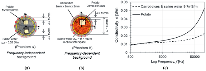
Figure 3. Phantom condition of (a) frequency-independent background and (b) frequency-dependent background. (c) Comparison of the electrical properties of phantom component materials.
Download figure:
Standard image High-resolution image3.2.1. Phantom A: frequency-independent background object.
The experiment with this type of phantom was carried out to analyze the image reconstruction performance for separation between inclusion objects (potato dice of size 15 mm × 20 mm × 40 mm) and a frequency-independent background object (saline water) (see figure 3(a)). Even though the human body is a frequency-dependent background object, a frequency-independent background object is commonly used to show the image reconstruction performance in the simple condition. Thus, we still considered this phantom as an evaluation object.
3.2.2. Phantom B: frequency-dependent background object.
The frequency-dependent background object phantom consisted of a potato dice (20 mm × 20 mm × 40 mm) inserted into carrot dice as a background with saline water (having the σecf of extracellular fluid) used to fill in the spaces in the carrot dice inclusions as shown in figure 3(b). The size of the carrot dice was 2 mm × 2 mm × 2 mm (8 mm3) and they were softly packed to fill the sensor volume.
3.3. Numerical simulation method
To evaluate the effect of the unknown contact impedance variance, we employed finite element method (FEM) simulations based on COMSOL Multiphysics v4.3a with the electrical circuit and the electric current modules [41] and the free-noise condition. Figure 4 illustrates the equivalent circuit of the EIT sensor including the instrumental effect and the contact impedance variance which is used in the numerical simulation. Here, ρ (=1/σ) (Ω m) is resistivity and Ae is the area of the electrode of height h (mm) and length Le (mm). The length Le is the distance between the adjacent ith (transmitter) and j th (receiver) electrodes or the adjacent kth (transmitter) and lth (receiver) electrodes. Figure 4(a) shows the current pathway length De (as for example De,1 for m = 1 in figure 4(b)) which is the distance between points f and g. The values Ci = 10 pF and Ri = 5 MΩ represent the instrumental effect obtained according to the study of Zhang et al [42] and their absolute value depends on the data acquisition system. Zi, Zj , Zk and Zl are the contact impedances whose values are shown in the curve of figure 5. Meanwhile, Z5, Zx and Z6 are the impedances of the domain (the phantom). Using COMSOL Multiphysics, the electric current module is used to calculate the electrical potential distribution ϕ, whilst the electrical circuit module is used to calculate the instrumental effect and the contact impedance variance. The boundary and phantom conditions of the numerical simulation are similar to those used in the experimental studies.
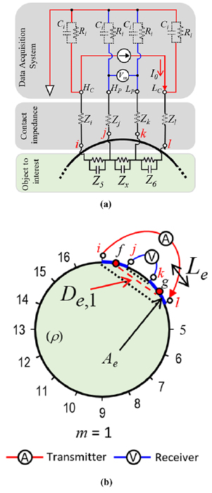
Figure 4. (a) The equivalent circuit of the four-wire measurement method in a circular sensor of EIT for (b) a single measurement including the instrumental effect and the contact impedance variance.
Download figure:
Standard image High-resolution image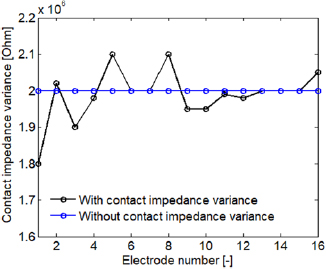
Figure 5. The contact impedance variance compared with a constant contact impedance.
Download figure:
Standard image High-resolution image3.4. Image reconstruction algorithm
The reconstructed images of conductivity change Δσ in experiments and numerical simulation studies were calculated using a total variation method, which is a hybrid between l2-norm- and l1-norm-based reconstruction methods. The reconstruction based on the total variation method is derived from the use of the following objective function [43]:
where  is the reconstructed conductivity change, n is the number of pixels, F is the forward solver used to predict the impedance data from Δσ, λ is the regularization parameter, which is calculated using the L-curve method, and L is the regularization matrix, of which LT · L = I, and I is the identity matrix. The L-curve displays a set of points with a representation that minimizes the first term
  versus the second term
  in the right-hand side of equation (12). The value of λ is selected at the maximum inflection point or the corner of the L-curve [44]. In order to solve equation (12), we use the total variation primal dual-interior point method (TV PD-IPM) [43]. Meanwhile, EIDORS v.3.9 package software is used to calculate the Jacobian matrix S using a homogeneous condition, with conductivity and permittivity values based on the phantom condition [45, 46]. In order to reconstruct the images of conductivity change Δσ, the frequency f a is fixed at 500 Hz, the lowest frequency measurement from the experiment. After that, f b was then changed and evaluated based on the reconstructed image.
3.5. Evaluation of image reconstruction performances
In this study the image reconstruction performances are evaluated using the values of RMSE, PE, RNG and SD [47]. The lower the value of the evaluation parameter the better the reconstruction performance.
RMSE (unitless) shows the aggregate residual value between the measured impedance and the predicted impedance:
Here ΔZ are the measured impedances from the experimental data while ΔZfem is the predicted impedance obtained from the FEM model based on the calculated Δσ.
PE (unitless) represents the accuracy of the reconstructed image in detecting the location of the inclusion:

r is the predicted center of the inclusion in the reconstructed image, while rtrue is the true location of the center of the inclusion in the phantoms.
RNG (unitless) represents the areas of opposite sign surrounding the inclusion of the reconstructed image:
Ain (mm2) is the area of inclusion in the reconstructed image. Aout (mm2) is the ringing, which is the area outside the inclusion in the reconstructed image that has an opposite sign to Ain (mm2).
SD (unitless) measures the ratio of the inclusion area in the reconstructed image Ain (mm2) which is not covered by the circular area Ac (mm2):
Ac is the circular area whose center is the center of inclusion in the reconstructed image, and the area of Ac is similar to Ain. The circular area is considered in this evaluation because a circle is the typical shape of the reconstructed image.
The correlation coefficient CC (unitless):
is used in the numerical simulation studies to quantify the effect of contact impedance variance. Δσw is the distribution of conductivity change when the electrode has contact impedance variance. Meanwhile, Δσo is the distribution of conductivity change when the electrode does not have contact impedance variance. The ideal value of CC is 1, which means the two conductivity distributions between Δσw and Δσo are identical.
4. Experimental results
4.1. Comparison of reconstructed images from experiments
As shown in figure 6, the inclusion object (i.e. potato dice area) of phantoms A and B based on conductivity change Δσ in fd-EIST and wfd-EIST is successfully reconstructed just as in the case of fd-EIT and wfd-EIT. The impedance changes ΔZ of fd-EIT, fd-EIST, wfd-EIT and wfd-EIST are acquired at f a = 500 Hz and f b = 2–6 kHz. The reconstructed images of phantom A produced by fd-EIST and wfd-EIST show a reasonably accurate inclusion shape, while those for fd-EIT and wfd-EIT show a relatively inaccurate inclusion shape (an ellipse-like shape). For phantom B, as shown in figure 7,the inclusion object geometry of fd-EIST and wfd-EIST is more consistent with the true shape of the inclusion compared with other reconstruction methods.
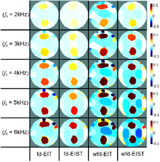
Figure 6. Effect of different frequencies f b on the reconstructed image of conductivity change Δσ (mS m−1) for phantom A.
Download figure:
Standard image High-resolution image
Figure 7. Effect of different frequencies f b on the reconstructed image of conductivity change Δσ (mS m−1) for phantom B.
Download figure:
Standard image High-resolution imageIn figures 6 and 7, fd-EIST and wfd-EIST show the interface boundary between the potato dice and carrot dice relatively consistently compared with fd-EIT and wfd-EIT, regardless of the frequency change, without suffering image artifacts. On the other hand, fd-EIT and wfd-EIT methods could not eliminate image artifacts, which look like an inclusion that appears inconsistently with changing frequency.
4.2. Evaluation of reconstructed images
4.2.1. RMSE.
For different frequencies f b, fd-EIST showed the lowest RMSE value (see figures 8(a) and 9(a)) compared with fd-EIT, wfd-EIT and wfd-EIST. As the frequency increased, all reconstruction methods showed an increasing RMSE value.
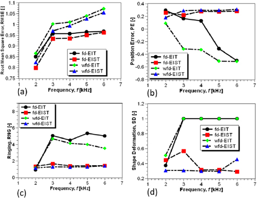
Figure 8. The evaluation of the reconstructed image of phantom A in terms of (a) RMSE, (b) PE, (c) RNG, (d) SD.
Download figure:
Standard image High-resolution image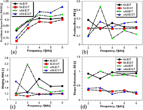
Figure 9. The evaluation of reconstructed image of phantom B in terms of (a) RMSE, (b) PE, (c) RNG, (d) SD.
Download figure:
Standard image High-resolution image4.2.2. PE.
The fd-EIST method showed the most consistent position of the inclusion in the reconstructed image for different frequencies for phantoms A and B compared with fd-EIT, wfd-EIT and wfd-EIST (see figures 8(b) and 9(b)). All reconstruction methods also showed errors in the position of inclusions in the reconstructed images.
4.2.3. RNG.
All reconstruction methods showed an area of ringing Aout that is greater than the area of the inclusion because the RNG values are higher than 1, as shown in figures 8(c) and 9(c). The fd-EIST method has the lowest RNG value and is almost constant for the different frequencies compared with fd-EIT, wfd-EIT and wfd-EIST for both phantom A and phantom B.
4.2.4. SD.
The SD value covered by the circular area Ac for methods fd-EIST and wfd-EIST was lower (about 70% lower for phantom A and about 60% lower for phantom B) compared with fd-EIT and wfd-EIT. Compared with fd-EIST, the SD value of wfd-EIST was more consistent for the different frequencies, as shown in figures 8(d) and 9(d). As shown by the result of figure 8(d), the SD of wfd-EIST is better than for the other reconstruction methods in terms of the boundary of the stability interface between the inclusion and background object for phantom A. Meanwhile, the SDs of fd-EIST and wfd-EIST are quite similar for phantom B.
4.3. Frequency-dependent behavior
Five different frequencies f b were used to evaluate the variance in the unknown contact impedance based on the frequency-dependent behavior, i.e. f b = 2, 3, 4, 5 and 6 kHz. For the ideal condition, i.e. without contact impedance variance, the curves of frequency-dependent behavior of conductivity change show that the conductivity change Δσ of the reconstructed images increases with increase in frequency [35]. If the frequency-dependent behavior curve shows an irregular change of Δσ for the reconstructed image with increasing frequency, the contact impedance variance is considered to influence the reconstructed image.
For phantom A, as shown in figure 10, fd-EIST and fd-EIT give the best performance. Figure 10 shows the curve of frequency-dependent behavior for four positions in the reconstructed images of phantom A shown in figure 6. Positions 1 and 2 are in the intracellular fluid of potato dice located in a biomaterial having a non-linear frequency-dependent behavior. All reconstruction methods showed an increase in the curve of frequency-dependent behavior with increasing frequency. In positions 1 and 2, fd-EIST and fd-EIT showed an approximate 30% increment in the curve of frequency-dependent behavior. Positions 3 and 4 are in the saline water (a frequency independent-background that is supposed to remain constant as the frequency increases). fd-EIST and fd-EIT showed an increment of less than 5% in the curve of frequency-dependent behavior. Meanwhile, wfd-EIST and wfd-EIT showed an increment of about 10%–20% in the curve of frequency-dependent behavior.
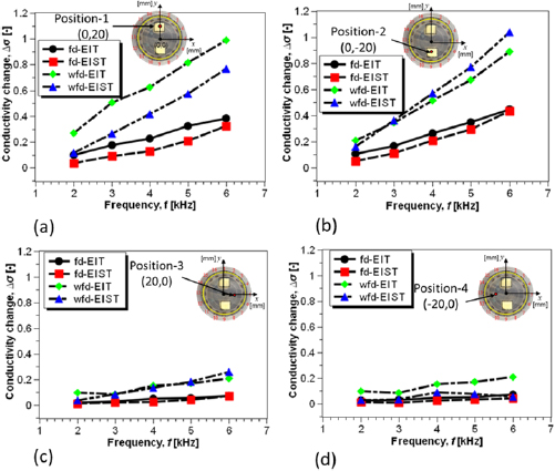
Figure 10. Frequency-dependent behavior at four different locations in the reconstructed image for phantom A: (a) position 1, (b) position 2, (c) position 3, (d) position 4.
Download figure:
Standard image High-resolution imageMeanwhile, for phantom B (figure 11), fd-EIST showed the most consistent frequency-dependent behavior curve in all positions compared with other reconstruction methods. Figure 11 shows the curve of frequency-dependent behavior for four positions in the reconstructed images of phantom B shown in figure 7. Position 1 is located in a biomaterial which has a non-linear frequency-dependent behavior. Positions 2, 3 and 4 are also considered to be in a biomaterial which has a different frequency-dependent behavior from position 1. Position 1 is in the intracellular fluid of potato dice while positions 2, 3 and 4 are in the frequency-dependent background objects (saline water and carrot dice). For position 1, all the reconstruction methods showed an increasing frequency-dependent behavior curve with increasing frequency. However, each reconstruction method showed a different degree of increment. wfd-EIST showed the highest increment while fd-EIT had the lowest increment of the four reconstruction methods. In ideal conditions the curve of frequency-dependent behavior in positions 2, 3 and 4 should show similar degrees of increment as the frequency increases. Among the four reconstruction methods, fd-EIST showed the results closest to ideal, with a 15% increment. fd-EIT produced a frequency-dependent behavior curve which tended to be constant.
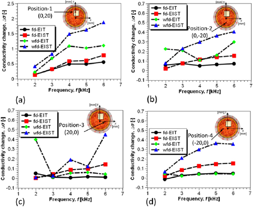
Figure 11. Frequency-dependent behavior at four different locations in the reconstructed image for phantom B: (a) position 1, (b) position 2, (c) position 3, (d) position 4.
Download figure:
Standard image High-resolution image5. Numerical simulation results
5.1. The effect of unknown contact impedance variance
Figure 12(a) shows that the unknown contact impedance variance affects the ideal trend line of the real part of impedance R from all measurements m. The effect of unknown contact impedance variance can be seen in the results of the numerical simulation comparing ΔZ for homogeneous conditions with the carrot dice background condition. Figure 12(a) shows the comparison of ΔZ without and with contact impedance variance evaluated at frequencies f a = 500 Hz and f b = 2 kHz, and figure 12(b) shows the change in ΔZ due to contact impedance variance.

Figure 12. The effect of unknown contact impedance variance is analyzed by comparing the real part of the impedance change ΔZ for homogeneous conditions with the numerical calculation which has constant contact impedance variance. (a) Comparison of impedance change for cases without, ΔZwo, and with, ΔZco, contact impedance variance. (b) The change of ΔZ due to contact impedance variance (ΔZwo − ΔZco).
Download figure:
Standard image High-resolution image5.2. Comparison of reconstructed images from numerical simulations
5.2.1. Phantom A: frequency-independent background object.
As shown in figure 13 for phantom A, fd-EIST had the ability to overcome the contact impedance variance better than fd-EIT, wfd-EIT and wfd-EIST. The existence of contact impedance variance significantly affects the accuracy of reconstructed images based on fd-EIT and wfd-EIT. As the frequency increases, the separation between potato dice inclusions becomes easier to distinguish. However, qualitative analysis based on reconstructed images is subjective from the user's point of view. Thus, we evaluated the correlation coefficient CC with and without contact impedance variance, as shown in the curve of figure 14. The CC value of fd-EIST is relatively higher than that for fd-EIT, wfd-EIT and wfd-EIST. Even though the CC value increases with frequency f b there is a trade-off between CC value and accuracy of the reconstructed image in terms of RMSE, PE, RNG and SD as shown in the experimental results.
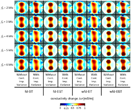
Figure 13. Comparison of the reconstructed images of phantom A without and with contact impedance variance based on numerical simulations.
Download figure:
Standard image High-resolution image
Figure 14. Correlation coefficient of phantom A without and with contact impedance variance based on numerical simulations.
Download figure:
Standard image High-resolution image5.2.2. Phantom B: frequency-dependent background object.
For phantom B, as shown in figure 15, the existence of contact impedance variance affects the accuracy of reconstructed images in a very similar way to that seen in figure 13. The CC values with fd-EIST and wfd-EIST are relatively higher than with fd-EIT and wfd-EIT, but tend to decrease as frequency f b increases, as shown in figure 16. Both fd-EIST and wfd-EIST depend on χnorm, which is calculated based on the resistance of the extracellular fluid Recf. According to the Cole impedance model, the resistance of the extracellular fluid Recf is acquired when the current flows only in the extracellular fluid. In this case, the current flowing through CPEm is negligible. We therefore hypothesize that fd-EIST and wfd-EIST are only accurate when the effect of permittivity change Δεr on impedance Z is relatively low compared with the effect of conductivity change Δσ at two sequential frequencies f a and f b.

Figure 15. Comparison of reconstructed images of phantom B without and with contact impedance variance based on numerical simulations.
Download figure:
Standard image High-resolution image
Figure 16. Correlation coefficient for phantom B without and with contact impedance variance based on numerical simulations.
Download figure:
Standard image High-resolution image6. Discussions
6.1. The volatile-distributed current source
We begin our discussion with an explanation of how variance in the unknown contact impedance causes the volatile-distributed current I1. Unknown contact impedance variance means that the value of contact impedance is not known prior to the experimental measurements. The volatile-distributed current I1 is analyzed via the impedance change based on a Kirchhoff loop analysis of figure 17, which shows an equivalent circuit of the four-wire measurement method. Zie is the capacitive coupling impedance. Zie = −j /(ωCi), where Ci is the capacitive coupling between voltmeter wires (Hp and Lp) and the virtual ground that causes impedance artifacts [48]. Zi, Zj , Zk and Zl are the variance contact impedances, where Zi ≠ Zj ≠ Zk ≠ Zl. Note that contact impedance has a frequency-dependent behavior, so it is represented as a parallel combination between the resistive and capacitive components. Zm is the measured impedance of the object of interest, Vx is the measured voltage of the object of interest, I0 is the injected current and Z5 and Z6 are the edge impedances due to the separation between electrodes. In the ideal case, I3 should be negligible because the input impedance of the voltmeter is very high. Therefore, analysis of the voltage of the object of interest Vx should be considered with I1:
where  . In loop I1:

Figure 17. Kirchhoff loop analysis of the equivalent circuit of the four-wire measurement method in a circular EIT sensor for a single measurement.
Download figure:
Standard image High-resolution imageBased on equation (19), the contact impedance variances Zk and Zl have a greater effect on the intensity of the value of I1 compared with Z6. In the ideal case, the value of I1 is constant for all the measurements. For the EIT measurement, the electrode combination k and l changes in all measurements, and the values of Zk and Zl also change among the electrodes. Therefore, the value of I1 also changes in all measurements, or a volatile-distributed current occurs.
The numerical simulation results shown in figures 12, 13 and 15 provide an understanding of the existence of unknown contact impedance affecting the impedance change ΔZ and the accuracy of the reconstructed images. Even though the numerical simulation could not mimic the experimental conditions perfectly, the equivalent circuit of the four-wire measurement method in a circular EIT sensor (as shown in figure 4) is capable of showing the effect of unknown contact impedance artificially. Generally, a comparison of the experimental and numerical simulation results leads us to conclude that the contact impedance variance causes the volatile-distributed current I1.
6.2. Frequency-dependent behavior
fd-EIST and wfd-EIST show better performances than fd-EIT and wfd-EIT because the reconstructed images have a frequency-dependent behavior that is closer to ideal. The volatile-distributed current I1 distorts the ideal frequency-dependent behavior of the object of interest. Non-ideal frequency-dependent behavior of the object of interest, as shown in figures 10 and 11, causes inaccurate calculation of the impedance change ΔZ in fd-EIT and wfd-EIT. In order to compensate for the volatile-distributed current I1 in the object of interest, a weighted parameter vector χnorm is used in fd-EIST and wfd-EIST to relate the sensor geometry and the current pathway length De for all the measurements m, as shown in figure 18. Figure 18 shows χnorm versus the measurement number list for one rotation of impedance measurement. The value of χnorm provides not only information about the sensor geometry but also the spatial condition of the inclusion object that is represented as the current pathway length. The green-dashed line gives information about the sensor geometry, which is the normalized linear distance between the transmitter and receiver electrodes  e, i.e. the lengths shown as red lines in the circle in figure 18. As shown in figure 18, χnorm has comparable characteristics for each background condition. χnorm functions as a baseline impedance value for synchronization and to signify the measured impedance from the inclusion object. This study gives a two-dimensional view of the reconstructed image, but we realize that the current pathway length has a three-dimensional distribution. In this regard, further analysis is needed to describe the behavior of χnorm for a three-dimensional sensor.
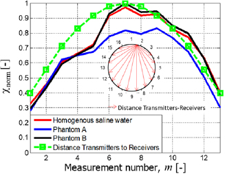
Figure 18. Comparison of the value of χnorm versus De from experimental studies.
Download figure:
Standard image High-resolution imageIn the reconstructed image, the color intensity depends on how different the real part of the impedance R is from the impedance at two sequential frequencies f a and f b, i.e. Ra − Rb. As Ra − Rb increases, the intensity of the color of the reconstructed image also increases. Meanwhile, the location of the interface boundary between the inclusion and background object depends on how the measurement number m experiences the change in impedance ΔZ. If the change in ΔZ is measured inaccurately the position of the interface boundary between the inclusion and the background object will be incorrectly recorded as the frequency changes. Figure 19 shows χnorm calculated from the conditions of phantom B. Even though the change in impedance ΔZ is recognized by using just two sequential frequency impedances, i.e. Ra − Rb, it is difficult to distinguish between the sources of the measured impedance because of the volatile-distributed current I1. A weighted function ξ of wfd-EIT is used to represent the measured impedance from the background object. The value of ξ depends on the selection of f b as shown in equation (5), and the accuracy of the reconstructed image depends on the accuracy of the prior information about the baseline impedance value of the background object. In a real situation, obtaining prior information about the background object is not a trivial task and can only be achieved by an invasive method, making it difficult to use EIT for functional imaging. In the proposed method χnorm can overcome the difficulties with wfd-EIT; it behaves as a weighted parameter vector of the real part of the impedance at two sequential frequencies. Compared with wfd-EIT, weighted parameters in fd-EIST and wfd-EIST do not depend on the selection of f b. Thus, fd-EIST and wfd-EIST do not need prior information about the background object.

Figure 19. The effect of the weighted parameter χnorm.
Download figure:
Standard image High-resolution image
Traditionally, fd-EIT or wfd-EIT reconstructs the interface boundary between an inclusion and background object as a representation of the change in physiological conditions. The unknown contact impedance variance limits the ability of fd-EIT or wfd-EIT to show more features. Taking the frequency-dependent behavior into consideration in the analysis of the reconstructed image improves physiological analysis by increasing the accuracy of interpretation in long-term monitoring applications. In long-term monitoring, the spatial as well as the temporal distribution of the abnormal physiological condition is detected. For the temporal distribution, characterization of the region considered to represent the abnormal physiological condition can be done by analyzing the frequency-dependent behavior.
7. Conclusions
In this paper have we proposed a weighted parameter vector, χnorm, for image reconstruction of conductivity change, Δσ, in order to simultaneously compensate for the volatile-distributed current due to variance in the unknown contact impedance in EIT. χnorm is based on extracellular fluid resistance via the Cole impedance model because the current pathway length  e is proportional to the real part of the impedance of the object of interest at zero frequency.
  e is considered in the reconstruction method because it reflects the volatile-distributed current I1 due to variance in the contact impedance. We applied χnorm to the EIT reconstruction methods fd-EIST and wfd-EIST, which are modifications of fd-EIT and wfd-EIT, respectively. Experimental phantom studies and numerical simulations were conducted using frequency-independent and frequency-dependent objects in order to evaluate the performance of fd-EIST and wfd-EIST compared with fd-EIT and wfd-EIT.
Based on the results and evaluation of the reconstructed images, it can be concluded that using the weighted parameter vector χnorm has the following merits.
- (1)fd-EIST has a root mean square error (RMSE) 12.5% lower than that of fd-EIT, while wfd-EIST has a RMSE 8.5% lower than wfd-EIT with χnorm.
- (2)fd-EIST is the most consistent reconstruction method with regard to the position error (PE) of the inclusion in the images at different frequencies. Both fd-EIST and wfd-EIST have PE values 60% lower than those of fd-EIT and wfd-EIT.
- (3)fd-EIST has the lowest ringing (RNG) value, which is almost constant at the different frequencies. The RNG values for fd-EIST and wfd-EIST are 80% and 77.78% lower than the values for fd-EIT and wfd-EIT, respectively.
- (4)With regard to shape deformation (SD), fd-EIST is most consistent of all the reconstruction methods with regard to the geometry of the inclusion at different frequencies. The SDs of fd-EIST and wfd-EIST are 70% lower than the values for fd-EIT and wfd-EIT, respectively.
- (5)fd-EIST is the best reconstruction method for the frequency-dependent behavior of the inclusion and background objects.
In this study, we evaluated the application of a weighted parameter vector χnorm for image reconstruction with conductivity change Δσ. However, we realize that it can also be applied in the evaluation of image reconstruction due to permittivity change Δε and therefore this concept will be looked at in our future studies.
Acknowledgments
This work was supported in part by an International Research Fellowship under Postdoctoral Fellowship of Japan Society for the Promotion of Science (JSPS) for Research in Japan (Standard) for the author Marlin Ramadhan Baidillah (Graduate School of Science and Engineering, Chiba University) and JSPS KAKENHI Grant Number JP18F18060. The authors would like to thank Martin Wekesa Sifuna (Doctoral Student in the Graduate School of Science and Engineering, Chiba University) for suggestions and revisions in this paper.