
Abstract
In recent years, higher-order topological phases have attracted great interest in various fields of physics. These phases have protected boundary states at lower-dimensional boundaries than the conventional first-order topological phases due to the higher-order bulk-boundary correspondence. In this review, we summarize current research progress on higher-order topological phases in both crystalline and non-crystalline systems. We firstly introduce prototypical models of higher-order topological phases in crystals and their topological characterizations. We then discuss effects of quenched disorder on higher-order topology and demonstrate disorder-induced higher-order topological insulators. We also review the theoretical studies on higher-order topological insulators in amorphous systems without any crystalline symmetry and higher-order topological phases in non-periodic lattices including quasicrystals, hyperbolic lattices, and fractals, which have no crystalline counterparts. We conclude the review by a summary of experimental realizations of higher-order topological phases and discussions on potential directions for future study.
Export citation and abstract BibTeX RIS

Original content from this work may be used under the terms of the Creative Commons Attribution 4.0 license. Any further distribution of this work must maintain attribution to the author(s) and the title of the work, journal citation and DOI.
1. Introduction
Quantum phases of matter, according to Landau's paradigm, were believed to be classified based on the symmetry of the ground state for a long time. However, in 1980, the discovery of quantum Hall effect showcased the example of topological phases of matter, for which different phases cannot be distinguished by spontaneously symmetry breaking but are characterized by the bulk topology [1, 2]. In 1988, the famous Haldane model was proposed to describe a topological insulator (TI) with quantum Hall conductance resulted from chiral edge states, which is characterized by a nonzero Chern number of bulk wave functions [3]. The connection between nontrivial bulk topology and topologically protected boundary states is referred to as bulk-boundary correspondence of TIs. Later, inspired by the discovery of time-reversal-invariant TIs [4–7], the concept of TIs has been extended to symmetry-protected topological states which are protected by either internal symmetries or spatial symmetries [8–15]. The symmetry-protected TIs cannot be adiabatically deformed into trivial insulators without closing the bulk gap if the symmetry is not broken, and they can be classified based on homotopy theory [16–18] and symmetry indicators based on band representations developed for topological crystalline insulators [19–21]. Besides TIs, people have also discovered topological superconductors described by gapped mean-field Hamiltonian [22–24] and topological semimetals with topological gapless points and protected surface states [25–28]. During the past decades, the topological phases of matter have attracted broad research interest and become a very active field in condensed matter physics [29–33].
The conventional topological phases in d dimensions host  -dimensional boundary states according to the bulk-boundary correspondence [9, 10]. In recent years, a new type of topological phases dubbed higher-order topological insulators (HOTIs) were discovered, for which a d-dimensional nth-order topological phase supports
  -dimensional boundary states with the codimension n > 1 [34–75]. In 2017, Benalcazar et al generalized the concept of the dipole moment to the multipole moment and proposed a model for multipole TIs protected by mirror symmetries, now known as the Benalcazar–Bernevig–Hughes (BBH) model, which exhibits quantized multipole moment and in-gap corner modes as the defining signature of higher-order topology [34, 35]. Specifically, a two-dimensional (2D) quadrupole TI is featured by quantized edge polarizations and fractional corner charges resulted from corner modes. The corner modes arise as the manifestation of nontrivial topology of edge Hamiltonians and cannot be removed by symmetry-preserving perturbations unless the bulk or edge energy gap closes [34, 35, 67, 70]. Analogously, an octupole TI is a three-dimensional (3D) third-order TI with the quantized octupole moment and corner modes [34]. In fact, it is not always true that a quadrupole TI always has corner modes. For instance, very recently, a quadrupole TI (with nonzero quadrupole moment) without corner modes in the energy spectrum has been found [76, 77].
Soon after the discovery of the multipole TIs, several works discovered 3D HOTIs with gapped surface states but gapless hinge states, in contrast to first-order TIs with gapless surface states [36–38]. In the absence of time-reversal symmetry (TRS), a typical class of second-order topological insulators (SOTIs) is featured by chiral hinge states, which can be protected by the product of time-reversal and rotational symmetry such as the  symmetry [38]. In the presence of TRS, there exist Kramers pairs of hinge states, namely, helical hinge states, which can be protected by additional crystalline symmetry such as mirror or rotational symmetry [36–38]. These gapless hinge modes give rise to quantized conductance, which is the transport signature of the higher-order topology. For many HOTIs with crystalline symmetry, the anomalous boundary states can be understood as the domain walls between massive Dirac Hamiltonians of adjacent gapped surfaces with opposite signs of masses due to the symmetry constraints [50]. In fact, in an early study on 3D topological superfluid 3He-B [78], it was found that in the presence of magnetic fields, the surfaces become gapped while there exists one-dimensional (1D) gapless modes at the line between different domains with opposite signs of the mass term due to magnetic field. Later, in two studies [79, 80], similar in-gap hinge modes were also found in 3D TIs, where the surface states are gapped out by the magnetic field or magnetization breaking the TRS. The chiral hinge modes emerge at the interface of adjacent surfaces with opposite signs of magnetic gaps. However, according to higher-order bulk-boundary correspondence proposed in [50], these higher-order topological phases (HOTPs) depending on the surface orientations or lattice terminations belong to extrinsic HOTPs, in contrast to intrinsic HOTPs originating from the nontrivial bulk topology protected by crystalline symmetry. The concept of higher-order topology has also been extended to higher-order topological superconductors hosting Majorana modes at corners or hinges [81–111], and higher-order topological semimetals hosting gapless points and Fermi arcs at hinges [112–124].
Since the pioneering works reporting HOTIs, it has witnessed a rapid development of both theoretical and experimental research in this field, and many models with higher-order topology were studied [34–74, 76–124]. For example, in 2Ds, the SOTIs with corner modes were found in breathing kagome and pyrochlore lattices, which are characterized by the quantized bulk polarizations [40]. In [59], the authors systematically investigated 2D SOTIs with quantized fractional corner charges protected by rotational symmetries. Moreover, several works studied fractional charge responses to topological defects such as dislocations and disclinations, which are related to higher-order bulk topology [125–130]. In 3Ds, it was found that HOTIs with anomalous hinge states can be protected by various crystalline symmetries including inversion symmetry, rotational symmetry, and magnetic symmetry such as  [44–51]. In addition, the space-time inversion symmetry (spinless PT symmetry) can protect 2D fragile topology with corner modes and 3D nodal-line semimetals with hinge Fermi arcs [53, 54, 113, 122]. Very recently, a Klein-bottle HOTI with non-chiral hinge modes protected by a pair of momentum-space glide reflection symmetries has been found [131].
In the presence of crystalline symmetry, HOTIs can usually be detected by symmetry indicators [37, 48, 59]. On the other hand, the higher-order topology can also be characterized by some bulk topological invariants. For instance, the 2D quadrupole TIs are characterized by the quadrupole moment as a  topological invariant [132, 133]. It was proved that the quadrupole moment is quantized by chiral symmetry [134, 135] or particle-hole symmetry [135]. The
  symmetric SOTIs with chiral hinge modes can be characterized by the Chern–Simons invariant [38]. Later, it was found that these chiral hinge modes can be also characterized by the winding number of the quadrupole moment [136, 137]. For the SOTIs with TRS, the helical hinge states can be characterized by the mirror Chern number in the presence of mirror symmetries [38]. In the absence of mirror symmetries, the helical modes can be characterized by a
  invariant proposed in [137]. Remarkably, either the quadrupole moment winding for chiral modes and the
  invariant for helical modes do not require the presence of crystalline symmetries. Therefore, both the 2D quadrupole TIs and 3D chiral or helical SOTIs can exist in systems without any crystalline symmetry.
People have also studied the effects of quenched disorder on the higher-order topology, and found that the higher-order topological states remain robust against weak disorder [34, 68, 95, 134, 135, 138–147]. More remarkably, the disorder is not always detrimental to topological phases. In two works studying quadrupole TIs in the presence of quenched disorder, it was found that disorder can induce a topological phase transition from a trivial insulator to a quadrupole TI with nonzero quadrupole moment quantized by chiral symmetry [134, 135]. The HOTP induced by disorder is named higher-order topological Anderson insulator, following the topological Anderson insulator found in first-order topological phases [148]. In an earlier study [95], the authors studied a second-order topological superconductor with Majorana corner modes and found that an initially trivial phase can transition into a HOTP upon adding disorder. The disorder-driven topological phase transitions can be explained by the renormalization of Hamiltonian parameters due to disorder. A subsequential study [149] considered a modified Haldane model with disorder in the hopping phases and found that the disorder can drive a transition from a Chern insulator to a HOTI with corner states, which was further observed in experiment.
Apart from crystals, recent years have witnessed the rapid progress on topological phases in non-crystalline systems lacking translational symmetries, where the conventional topological band theory is not applicable. One typical category of non-crystalline systems discovered in nature are quasicrystals, which have no translational symmetry but still possess quasi long-range order [150]. A quasicrystalline lattice can usually be viewed as a projection of a higher-dimensional lattice. In 2Ds, quasicrystals can respect rotational symmetry forbidden in periodic crystals, such as five-fold or eight-fold rotations. A number of topological phases have been studied in quasicrystals [151–166]. Another large class of non-crystalline systems is amorphous systems, which have no any crystalline symmetry and no long-range order [167]. In nature, there exist abundant materials belonging to amorphous systems, for instance, the glass-like materials. An amorphous system can be modeled as a lattice composed of randomly distributed sites, which can be generated upon adding structural disorder to a regular lattice. Despite the lack of any spatial symmetry, there have been an amount of topological phases reported in amorphous systems [168–210]. In addition to these two relatively real systems, people have also studied topological phases in other artificial non-periodic structures, including fractal lattices [211–219] and hyperbolic lattices [220–222]. Fractals exhibit self-similar structures with non-integer dimensions [223]. Remarkably, though introduced in mathematics, fractal structures have been observed in real materials recently [224]. Hyperbolic lattices live in the hyperbolic plane of negative curvature, which can be partly described by hyperbolic band theory [225]. As will be introduced in the following, these non-crystalline systems can also harbor a variety of HOTPs, including topological phases without crystalline counterparts.
Specifically, the authors in [226] showed that a HOTI with quantized quadrupole moment and zero-energy corner modes can exist in a 2D amorphous system, for which the higher-order topology is actually protected by chiral symmetry. Later, the authors in [137] found SOTIs with either chiral or helical hinge states in a 3D amorphous system, which are characterized by nontrivial topological invariants, quantized longitudinal conductance, and in-gap hinge states. More intriguingly, it was found that the structural disorder can induce a SOTI starting from a trivial insulator on a regular lattice. The topological phase transition occurs through a bulk energy gap closure guaranteed by an average  symmetry. Recently, it has been realized that the average symmetry plays an important role in the classification of symmetry-protected topological phases [227].
Apart from amorphous systems without any spatial symmetry, the HOTPs with in-gap corner modes have been found to exist in other non-crystalline systems such as quasicrystalline [228–237], hyperbolic [238, 239], and fractal lattices [213, 224, 240–244]. Since quasicrystalline and hyperbolic lattices can possess rotational symmetries that do not exist in regular crystals, they can harbor topological phases without crystalline counterparts. For instance, it was found that a HOTP hosting eight corner modes exists in a quasicrystal with eight-fold rotational symmetry, which can be characterized by a  invariant protected by particle-hole symmetry [228, 229]. Similar phases were also found in 2D amorphous lattices with an average rotational symmetry [245] and hyperbolic lattices with various rotational symmetries [238, 239]. In [246], the authors studied a 3D quasicrystalline lattice constructed by stacking 2D quasicrystals and found a 3D SOTI with eight hinge states or helical pairs of hinge states. It was found that these phases are protected by the winding number of the generalized quadrupole moment and a
  invariant based on transformed lattice sites, respectively. The authors also shown that the 2D HOTI on a quasicrystalline lattice can be characterized by the generalized quadrupole moment [246].
There have been several papers reviewing the topics of HOTPs in crystalline systems. In [50, 247], the authors introduced the general theory of higher-order bulk-boundary correspondence to classify the bulk and boundary topology of HOTPs, mainly for HOTPs protected by crystalline symmetry. Another excellent review [248] introduced celebrated models of HOTPs and especially focused on experimental realizations in various classical platforms, such as metamaterials and electric circuits. Both of them have focused on HOTPs in crystalline systems, which can be well understood using conventional topological band theory. In comparison, our review includes HOTPs in both crystalline and non-crystalline systems and can be roughly divided into two parts. The first part introduces several prototypical models for HOTPs in crystalline systems. We demonstrate the higher-order boundary states of these models and present corresponding topological invariants beyond symmetry indicators, which have not been reviewed in detail before. The second part discusses HOTPs in systems with quenched disorder and various kinds of non-crystalline systems lacking translational symmetry, which have not been covered in previous reviews. We have comprehensively reviewed the research progress on HOTPs in disordered and non-crystalline systems including amorphous, quasicrystalline, hyperbolic, and fractal lattices.
The review is organized as follows. In section 2, we review several prototypical models of HOTPs in crystals and introduce their topological properties. In section 3, we review the studies on disorder effects on HOTPs and demonstrate disorder-induced HOTPs. In section 4, we review the studies on HOTPs in non-crystalline systems including amorphous lattices, quasicrystalline lattices, hyperbolic lattices, and fractal lattices. In section 5, we briefly summarize the experimental progress on HOTPs in both solid state materials and metamaterials. Finally, in section 6, we give a summary and perspective.
2. Higher-order topological phases in crystalline systems
In this section, we will review several prototypical models of HOTPs, including multipole TIs, chiral-symmetric HOTPs, 3D HOTIs with chiral or helical hinge modes, and higher-order topological semimetals.
2.1. Multipole topological insulators
Here we will introduce a class of HOTPs named quantized electric multipole insulators or multipole TIs. They are characterized by quantized multipole moment and zero-dimensional corner states, which are generalizations of 1D TIs with quantized polarization. We mainly focus on a prototypical model of quadrupole TIs known as the BBH model (see figure 1(a)) proposed in [34], and discuss its bulk and boundary properties and corresponding topological invariants. The model for octupole TIs can be constructed analogously (see figure 1(b)), which belongs to third-order topological phases [34].

Figure 1. (a) Schematic illustration of the 2D BBH model with quantized octupole moment where γ and λ represent intracell and intercell hopping, respectively. The dashed lines represent the hopping terms with negative signs. The numbers indicate the basis for Γ matrices (see equation (2)). (b) Schematic of the tight-binding model with quantized octupole moment.
(c) The energy spectrum of the BBH model with open boundary conditions along x and y as a function of  with
with  and
and  . The red lines describe four degenerate corner states. (d) Schematic illustration of the BBH model in a limiting case with
  , showing how corner states and edge polarizations arise. (e) The phase diagram of the BBH model defined in equation (2), where QTI represents the quadrupole topological insulating phase. The phase transition between the QTI phase in yellow region and trivial phase in white and grey region occurs when either the bulk energy gap closes at the red points or the edge energy gap closes at the blue lines. (a)–(c) From [34]. Reprinted with permission from AAAS.
Download figure:
Standard image High-resolution image2.1.1. Benalcazar-Bernevig-Hughes model.
The BBH model is a tight-binding model on a square lattice [34, 35]

where  (
( ) with
  are creation (annihilation) operators for the four sites within a unit cell labelled by r, as shown in figure 1(a). Here,
  and
and  are lattice vectors. We take lattice constants
  .
.  and
and  are nearest-neighbor hopping amplitudes. In momentum space, the corresponding Bloch Hamiltonian is

where  ,
,  ,
,  ,
,  are mutually anticommuting Hermitian matrices [34, 35]. Here τj
, σj
are Pauli matrices representing the degrees of freedom within a unit cell. This model describes spinless electrons on a square lattice with π-flux per plaquette and the hoppings are dimerized along x and y directions. The Hamiltonian
are mutually anticommuting Hermitian matrices [34, 35]. Here τj
, σj
are Pauli matrices representing the degrees of freedom within a unit cell. This model describes spinless electrons on a square lattice with π-flux per plaquette and the hoppings are dimerized along x and y directions. The Hamiltonian  has two energy bands and each band is two-fold degenerate enforced by the TRS and inversion symmetry (see the following proof). The model is an insulator at half filling unless the bulk energy gap closes at
  .
.
The Hamiltonian (2) satisfies two mirror symmetries  and
and  represented by
  and
and  , respectively,

with  and
and  . When
  and
and  , the Hamiltonian (2) respects a four-fold rotational symmetry C4 with
  ,
,

where  and
and  . The Hamiltonian (2) also has spinless TRS
  represented by the complex conjugation κ, particle-hole symmetry
  represented by
  , and chiral symmetry
  represented by
  [34].
[34].
We now prove that the TRS and the inversion symmetry  , which anticommute with each other, guarantee that each energy band is at least two-fold degenerate. Let
  be an eigenstate of the Hamiltonian (2) with the energy
  at
k
. Then
at
k
. Then  corresponds to an eigenstate with the same energy at
k
. Assume that there were no degeneracy at
k
, which is equivalent to saying that the two states refer to the same one up to a phase θ, i.e.
corresponds to an eigenstate with the same energy at
k
. Assume that there were no degeneracy at
k
, which is equivalent to saying that the two states refer to the same one up to a phase θ, i.e.  . Using
  , we obtain
  . On the other hand, due to the anticommutation relation of UI
and
. On the other hand, due to the anticommutation relation of UI
and  ,
,  , leading to
  , which is impossible. We therefore conclude that each energy band is at least two-fold degenerate.
Due to the π-flux in each plaquette, the mirror symmetries Mx
and My
anticommute with each other, namely,  , which guarantees the two-fold degeneracy of energy bands at high-symmetry points and leads to the gapped Wannier bands [34, 35]. The mirror symmetries or fourfold rotational symmetry can enforce the quantization of the bulk quadrupole moment qxy
(see definition in section 2.1.3).
, which guarantees the two-fold degeneracy of energy bands at high-symmetry points and leads to the gapped Wannier bands [34, 35]. The mirror symmetries or fourfold rotational symmetry can enforce the quantization of the bulk quadrupole moment qxy
(see definition in section 2.1.3).
Owing to the mirror symmetries, the BBH model has zero bulk polarization and zero Chern number so that there are no first-order edge states [34]. The absence of the Chern number can also be seen from the existence of the TRS. However, when  and
and  , the model supports zero-energy corner modes localized at four corners in the energy spectrum with full open boundary conditions (see figure 1(c)). For clarity, we consider a limiting case with
  to illustrate these nontrivial signatures for the quadrupole topological phase illustrated in figure 1(d). It is clear to see the existence of four isolated sites, contributing to four zero-energy corner modes. In addition, we also easily see that there is a 1D Su-Schrieffer-Heeger (SSH) chain with mirror symmetry localized at each edge, which yields a quantized polarization
  tangent to the edge. The quantized edge polarization comes from the nontrivial topology of the 1D boundary. The edge polarization of the 1D boundary also indicates the existence of boundary states of boundary, which form the corner modes.
In fact, in the entire topological region, the phase has a quantized bulk quadrupole moment  , quantized edge polarizations
  tangent to the boundaries along x and y, and zero-energy corner states [34]. The nontrivial phase is dubbed a quadrupole topological insulator (QTI). When
  or
or  , the model is topologically trivial without boundary signatures. Figure 1(e) shows the phase diagram of the BBH model with respect to the parameter ratios
  and
and  , which includes the topologically nontrivial QTI phase with
  and the trivial phase with
  . The quantization of the quadrupole moment is protected by the mirror symmetries or chiral symmetry (see section 2.1.3). The edge polarizations are the polarizations localized along the edges when we take a cylinder geometry with open boundary in x (y) and periodic boundary in y (x) (see section 2.1.5). The integrated polarization near one edge are quantized to
  by effective mirror symmetries inherited from the bulk. The edge polarization
  and
and  jumps to
  from zero as we change parameters
  and
and  across the phase boundaries at
  with
with  and
and  with
with  . This happens either through the edge energy gap closing or the Wannier gap closing of the Wannier bands (see section 2.1.4).
The BBH model can be generalized to 3Ds (see figure 1(b)), which is a model for octupole TIs with quantized octupole moment [34]. The model hosts eight zero-energy corner modes.
2.1.2. Corner modes and corner charges.
Here we will follow [34, 35] to give the analytic solution of the corner modes for the BBH model (2). For simplicity, we will solve a continuum model for the lattice Hamiltonian (2) by expanding the Hamiltonian near  and
and  where the bulk gap closes up to the first order,

where we take  and assume that
  and
and  . The parameters
  are small and are positive (negative) for the topological (trivial) phase of the BBH model. To solve the corner states under open boundary conditions, we introduce the edges normal to the x or y direction, namely, the x-edge or y-edge forming domain walls and change mx
and my
from positive to negative values across the domain walls. Note that for positive mx
and my
, the system is in a topological phase while for negative ones, it is in a trivial phase.
are small and are positive (negative) for the topological (trivial) phase of the BBH model. To solve the corner states under open boundary conditions, we introduce the edges normal to the x or y direction, namely, the x-edge or y-edge forming domain walls and change mx
and my
from positive to negative values across the domain walls. Note that for positive mx
and my
, the system is in a topological phase while for negative ones, it is in a trivial phase.
We first use the continuum model (5) to solve the states localized at the x-edge (x = 0) in the absence of y-edges. The wave function localized at the x-edge takes the form  where f(x) is a scalar function and
  is a spinor. We require the wave function to satisfy the Schrödinger equation,

where we replace kx
with  and ε is the eigenenergy. This equation has a solution
  and the spinor
  should satisfy the equation
  , i.e.
  . We have two solutions
  or
or  . We can project the Hamiltonian into the subspace of these edge states to obtain the low-energy effective Hamiltonian for the x-edge

where  are Pauli matrices in the basis
  . We can perform an analogous calculation for the y-edge and have the equation for the spinor
  , which has two solutions
  or
or  . Similarly, the y-edge Hamiltonian is obtained by projecting the Hamiltonian into the basis
  ,
,

where  are Pauli matrices in the basis.
Both of these edge Hamiltonians take the form of massive 1D Dirac models for a 1D TI with the 1D mirror symmetry. Now we consider a corner that is the intersection of the right x-edge and the upper y-edge. The zero-energy corner mode can be seen as either a y-domain wall of the x-edge or a x-domain wall of the y-edge, which have the identical solution as

Therefore, we have a single corner mode at each corner of a square geometry, which is a simultaneous eigenstate of both edge Hamiltonians.
In general, the boundary states of a HOTI can be understood from the view of domain walls of Dirac mass protected by crystalline symmetries [36–38, 50]. Here we illustrate this picture using a Dirac Hamiltonian form of the 2D BBH model with fourfold rotational symmetry. In the presence of the C4 symmetry ( and
and  ), the BBH Hamiltonian (2) can be rewritten in an alternative form of Dirac Hamiltonian [37],

by performing the transformations  ,
,  ,
,  , and
, and  ; these new matrices constitute a new set of Dirac matrices anticommmuting with each other. Meanwhile, we define the parameters
  and
and  . Similarly to the BBH model, this Hamiltonian has a HOTP with zero-energy corner modes protected by
  symmetry when
  and
and  [37].
[37].
Without the mass term, i.e.  , the Hamiltonian (10) has a TRS represented by
  , belonging to the class AII (time-reversal invariant topological insulator with spin). When
  , gapless helical edge state arise. The
  term breaks the TRS as well as the C4 rotational symmetry represented by
  , but preserves the symmetry of their combination. The breaking of the TRS leads to the opening of the gap of the helical modes, resulting in an effective mass for the edge Dirac Hamiltonian. Due to the
  symmetry, the Dirac mass of the edge Hamiltonian changes sign under a C4 rotation. Thus, there exists a domain wall at a corner between two edges related by the C4 rotation, which gives rise to a corner state. There are a total of four corner states for an open boundary compatible with the C4 symmetry.
The corner states lead to filling anomaly [70] or fractional charges [59, 249] localized at the corners. Specifically, if we require the system to be gapped and symmetric, it is inevitable to have the four degenerate corner states to be either totally occupied or totally unoccupied, resulting in excess fractional charges localized at each corner, which is the manifestation of filling anomaly. On the other hand, if we require the constraints of neutrality rather than symmetry, we can add an infinitesimal symmetry-breaking term in the Hamiltonian to break the degeneracy so that two diagonal corner states are occupied. As a result, fractional corner charges of either  or
or  occur near the corners.
In practice, the corner charge for one corner (similarly for the other three corners) is numerically calculated by performing the integration of the charge density over a quadrant of the system [35],

Here, ![$\rho(\textbf{R}) = 2e-e\sum_{n = 1}^{N_{\mathrm{occ}}}\sum_{\alpha = 1}^4|[u^{n}]^\mathbf{R,\alpha}|^2$](https://content.cld.iop.org/journals/0953-8984/36/28/283002/revision2/cmad3abdieqn120.gif) is the charge density. The first and second terms arise from the atomic positive charges and the electron distribution, respectively. The latter is calculated by the occupied state
is the charge density. The first and second terms arise from the atomic positive charges and the electron distribution, respectively. The latter is calculated by the occupied state  of the Hamiltonian under open boundary conditions (
![$[u^{n}]^\mathbf{R,\alpha}$](https://content.cld.iop.org/journals/0953-8984/36/28/283002/revision2/cmad3abdieqn122.gif) represents the αth component at the site R of the nth occupied state). For the corner charge computation, an infinitesimal term should be added to break the symmetry to lift the fourfold degeneracy of corner modes. In other words, two corner states have positve energy and the other two have negative energy. One thus can fill two negative corner states with electrons at half filling, leading to fractional corner charges of
represents the αth component at the site R of the nth occupied state). For the corner charge computation, an infinitesimal term should be added to break the symmetry to lift the fourfold degeneracy of corner modes. In other words, two corner states have positve energy and the other two have negative energy. One thus can fill two negative corner states with electrons at half filling, leading to fractional corner charges of  (we consider the existenc of positive charges of 2e in each unit cell).
The topological corner modes of the quadrupole TIs can also be probed by the in-gap modes of the nested entanglement spectrum [38, 67] or the entanglement spectrum between a quarter part and its complement [76]. In other words, for most models, both the energy spectrum of the Hamiltonian and the entanglement spectrum support in-gap corner modes in the topological region. However, Tao and coworkers propose a model Hamiltonian with a staggered  gauge field and find that this model leads to a quadrupole insulator without corner modes in the energy spectrum but with in-gap corner modes in the entanglement spectrum [76]. In fact, the entanglement spectrum has a one-to-one correspondence with the energy spectrum of the flattened Hamiltonian rather than that of the original Hamiltonian. When we change the flattened Hamiltonian to the original Hamiltonian by varying the eigenenergies, the edge energy gap closes and reopens, leading to the disappearance of the corner modes [76]. During this process, the bulk states remain unchanged so that the quadruple moment does not change.
2.1.3. Quadrupole moment as a topological invariant.
Here we review a real-space formula of the electric quadrupole moment and show that its value should be quantized in the presence of some crystalline symmetries or chiral symmetry. The formula of the quadrupole moment defined here may not correctly evaluate the physical quadrupole moment for a real system. There have been some discussions on the subtlety of proper definition of the bulk quadrupole moment [250–253]. Nevertheless, it can be used as an indicator for the second-order topology of quadrupole insulators like the BBH model.
The real-space quadrupole moment is defined by a generalization of the Resta formula for the electric polarization [254]. Proposed in [132, 133], the quadrupole moment qxy (in units of e) for a many-electron system is defined as

where  with
with  denoting the electron number operator at site
 ![${\boldsymbol{r}} = (x,y)\in(0,L_x]\times (0,L_y]$](https://content.cld.iop.org/journals/0953-8984/36/28/283002/revision2/cmad3abdieqn127.gif) in a system of size Lx
by Ly
.
in a system of size Lx
by Ly
.  denotes the average electron filling per unit cell counting the atomic positive charge contribution that we need to subtract.
  is the many-body ground state of electrons in a periodic system. Similar to the polarization from the Resta formula, the quadrupole moment qxy
is only defined in
is the many-body ground state of electrons in a periodic system. Similar to the polarization from the Resta formula, the quadrupole moment qxy
is only defined in  because of the periodicity of complex phases. Note that to have a well-defined quadrupole moment (invariance under translations), we require that the bulk polarizations vanish [34]. The octupole moment can be defined analogously by replacing
  with
with  [132, 133].
For noninteracting fermion systems, the many-body wave function can be written as a Slater determinant of occupied single-particle eigenstates. Then, it can be shown that the quadrupole moment is evaluated by [115, 134, 135]

where we define an  matrix
  representing the occupied states of an
  single-particle Hamiltonian under periodic boundary conditions.
  is an
is an  diagonal matrix [
 is the real-space coordinate of the jth degree of freedom]. Here, nc
is the total number of occupied states, and na
is the total dimension of the single-particle Hamiltonian. In the calculation, one also needs to deduct the contribution from background positive charge distribution, that is,
is the real-space coordinate of the jth degree of freedom]. Here, nc
is the total number of occupied states, and na
is the total dimension of the single-particle Hamiltonian. In the calculation, one also needs to deduct the contribution from background positive charge distribution, that is,  where
where  is the position of the jth positive charge.
We can apply the formula (13) to evaluate the quadrupole moment of typical models of quadrupole insulators. For the BBH model (2) with chiral symmetry, we have  for the quadrupole topological phase when
  are both in the interval
  . For the SOTI with
  symmetry in equation (10),
  when
when  and
and  , which correctly characterizes the topologically nontrivial phase with corner modes. Note that the quadrupole moment as a topological invariant can predict the topological phase transitions between the topological and trivial phases of quadrupole insulators when either the bulk energy gap or edge energy gap closes. In fact, the quadrupole moment characterizes the topology of the flattened Hamiltonian, and thus its topology manifests in the existence of in-gap corner modes in the flattened Hamiltonian or the entanglement spectrum [76]. For most models, the original Hamiltonian also supports corner states because it is connected to the flattened version without experiencing any edge energy gap closure. However, there exists a model where quadrupole insulators do not have corner states in the energy spectrum [76].
2.1.3.1. Quantization of qxy protected by crystalline symmetries.
Under mirror symmetry,  or
or  , we see that the operator
  in equation (12) transforms into
  . Thus, we have
  . If the system is invariant under the mirror transformation, we have
  so that qxy
takes the quantized value of either 0 or
so that qxy
takes the quantized value of either 0 or  . Similarly, we see that the four-fold rotation
  also flips the sign of qxy
. Thus, the C4 symmetry enforces that
also flips the sign of qxy
. Thus, the C4 symmetry enforces that  , indicating that qxy
is quantized in the presence of the C4 symmetry.
, indicating that qxy
is quantized in the presence of the C4 symmetry.
2.1.3.2. Quantization of qxy protected by chiral symmetry.
Apart from crystalline symmetries, the quadrupole moment can be quantized by internal symmetries alone. In the following, we present the proof of quantization of qxy
(13) protected by chiral symmetry by following [134, 135]. Let H be a generic single-particle Hamiltonian in real space preserving chiral (sublattice) symmetry, that is, there exists a unitury operator Π such that  . If we consider an occupied state
  with energy En
, then we can obtain an unoccupied state by applying Π to the occupied one, that is,
with energy En
, then we can obtain an unoccupied state by applying Π to the occupied one, that is,  with energy
  . Since the energy spectrum is symmetric about the zero energy, we consider the half-filling case with
  . Then, we have
  . The set
  therefore constitutes the unoccupied states. These unoccupied states can be represented by
  . The quadrupole moment (13) can be written as

Because the unitary matrix  commutes with the chiral (sublattice) symmetry transformation Π with
  , i.e.
 ![$\left[\hat{D},\Pi\right] = 0$](https://content.cld.iop.org/journals/0953-8984/36/28/283002/revision2/cmad3abdieqn167.gif) ,
,

Next, we will prove that  .
.
Proof. We define an  unitary matrix
  . It can be easily seen that
  . Then, we have the following relations

In the derivation, the following orthonormal properties are used,  ,
,  and
and  . □
. □
Therefore, we get the conclusion that  , namely, qxy
is quantized to 0 or
, namely, qxy
is quantized to 0 or  up to an integer. One can also apply the above procedure to prove that the octupole moment is quantized in 3Ds in the presence of chiral symmetry. Similar conclusion can be generalized to systems with particle-hole symmetry [135]. Since the chiral symmetry alone can protect the quantization of the quadrupole moment, we can have quadrupole TIs in disordered systems lacking crystalline symmetry [134, 135, 226].
2.1.4. Wannier bands and topological invariants.
Here we review the topological properties of Wannier bands for quadrupole insulators protected by mirror symmetries.
2.1.4.1. Wilson loop and Wannier band.
In general, we consider a Bloch Hamiltonian  which has
  degrees of freedom and
  occupied bands with Bloch functions
  for
for  . The Wilson loop is closely related to the position operator projected into the occupied space [254]. In the following, we will focus on the Wilson loop along kx
,
. The Wilson loop is closely related to the position operator projected into the occupied space [254]. In the following, we will focus on the Wilson loop along kx
,  , and the Wilson loop
  along ky
can be evaluated similarly. The Wilson loop
along ky
can be evaluated similarly. The Wilson loop  starting from the base point
  of the loop in Brillouin zone, is defined under full periodic boundary conditions as follows

where ![$[F_{x,{\textbf{k}}}]^{mn} = \left\langle u^{m}_\mathbf{k+{\delta} k_x} \right| \left. u^n_\textbf{k} \right\rangle$](https://content.cld.iop.org/journals/0953-8984/36/28/283002/revision2/cmad3abdieqn186.gif) , for
, for  . Since the Wilson loop is unitary in the thermodynamic limit, it can be defined as an exponential of a Hermitian matrix

Then, we refer to  as the Wannier Hamiltonian. It has been illustrated that the Wannier Hamiltonian's spectrum has a close connection with the spectrum and topology of the boundary perpendicular to the x direction [255].
The Wilson loop operator can be diagonalized as

where  is the eigenvectors with components
 ![$[\nu^{\,j}_{x,{\textbf{k}}}]^n$](https://content.cld.iop.org/journals/0953-8984/36/28/283002/revision2/cmad3abdieqn190.gif) for
for  . The Wannier Hamiltonian
  has eigenvalues
  ,
,  , which only depend on ky
of the base point k. The eigenvalues
, which only depend on ky
of the base point k. The eigenvalues  defined modulo 1 are referred to as the Wannier centers and compose the Wannier bands.
For the BBH model with two occupied bands, the phases  of the Wilson loop
  over two occupied bands form a pair of opposite values
  due to the mirror symmetry Mx
, leading to the vanishing of the bulk polarizations. The two Wannier bands
due to the mirror symmetry Mx
, leading to the vanishing of the bulk polarizations. The two Wannier bands  have a Wannier gap at both
  and
and  over the Brillouin zone. Therefore, we can have a 1D gapped Wannier Hamiltonian
  for
for ![$k_y \in [-\pi,\pi]$](https://content.cld.iop.org/journals/0953-8984/36/28/283002/revision2/cmad3abdieqn203.gif) , which may host nontrivial band topology.
, which may host nontrivial band topology.
2.1.4.2. Nested Wilson loop and Wannier-sector polarization.
When the Wannier bands  are gapped for
 ![$k_y \in (-\pi,\pi]$](https://content.cld.iop.org/journals/0953-8984/36/28/283002/revision2/cmad3abdieqn205.gif) , we can define two Wannier sectors separated by the gap. For quadrupole insulators with two anticommuting mirror symmetries Mx
and My
, the Wannier bands
, we can define two Wannier sectors separated by the gap. For quadrupole insulators with two anticommuting mirror symmetries Mx
and My
, the Wannier bands  are gapped for
 ![$k_y \in (-\pi,\pi]$](https://content.cld.iop.org/journals/0953-8984/36/28/283002/revision2/cmad3abdieqn207.gif) at both
at both  and
and  . Then, we can define two Wannier sectors
  and
and  . In the BBH case, there is only one band in each Wannier sector.
The topological invariant for a Wannier sector νx
can be evaluated based on the nested Wilson loops. With the Wannier bands  and Wilson loop eigenstates
  , the nested Wilson loop is a Wilson loop of one subspace of Wannier bands along ky
. Specifically, for the two Wannier sectors
, the nested Wilson loop is a Wilson loop of one subspace of Wannier bands along ky
. Specifically, for the two Wannier sectors  split by the Wannier gap, we define the Wannier band basis in the Wannier sector
  as
as

for  . NW
is the number of the Wannier bands in the sector
. NW
is the number of the Wannier bands in the sector  . This basis obeys
  . Then, the nested Wilson loop along y for the Wannier sector νx
over the Wannier band basis is defined as
. Then, the nested Wilson loop along y for the Wannier sector νx
over the Wannier band basis is defined as

where ![$[F^{\nu_x}_{y,{\textbf{k}}}]^{rs} = \left\langle w^r_{x,\textbf{k}+\mathbf{\delta k_y}} \right| \left. w^s_{x,{\textbf{k}}} \right\rangle$](https://content.cld.iop.org/journals/0953-8984/36/28/283002/revision2/cmad3abdieqn219.gif) with
with  over all Wannier bands in the Wannier sector νx
, and
over all Wannier bands in the Wannier sector νx
, and  . The total polarization of the Wannier sector νx
is
. The total polarization of the Wannier sector νx
is

which, in the thermodynamic limit, becomes an integral

where  is the Berry connection of Wannier bands νx
having components
is the Berry connection of Wannier bands νx
having components

where  run over the Wannier bands in Wannier sector νx
[34, 35].
run over the Wannier bands in Wannier sector νx
[34, 35].
Under the mirror reflection My
and Mx
, the Wannier-sector polarizations satisfy  and
and  , respectively [34, 35]. Hence,
  and
and  are quantized to 0 or
  . For the topological nontrivial phase of the BBH model (2), we have
  in consistent with the quadrupole moment
  . The transition between the phase with different Wannier-sector polarizations is driven by the gap closing of the Wannier bands.
The mirror symmetries can also simplify the computation of the topological invariants. Since the 1D Wannier Hamiltonian  is invariant under the mirror reflection My
inherited from the bulk, the Wannier-sector polarization can be obtained from the reflection eigenvalues of Wannier band basis (20) at mirror invariant momenta [34, 35].
is invariant under the mirror reflection My
inherited from the bulk, the Wannier-sector polarization can be obtained from the reflection eigenvalues of Wannier band basis (20) at mirror invariant momenta [34, 35].
2.1.4.3. Symmetry constraints of Wannier Hamiltonian.
Consider a generic Bloch Hamiltonian  with a symmorphic lattice symmetry g:
  , described by
  , where g is a unitary operator for the symmetry. We now define a Wilson line following a path C in momentum space from ki
to kf
as
, where g is a unitary operator for the symmetry. We now define a Wilson line following a path C in momentum space from ki
to kf
as

where ![$[F_\textbf{k}]^{mn} = \langle u_\mathbf{k+\delta k}^m|u_\textbf{k}^n\rangle$](https://content.cld.iop.org/journals/0953-8984/36/28/283002/revision2/cmad3abdieqn235.gif) with
with  labeling the occupied bands and
  . We take
  in the thermodynamic limit. The Wilson line operator transforms under the symmetry as [34, 35]

Here a unitary sewing matrix  is defined. The matrix reflects the connection between eigenstates at k with eigenstates at
  . In particular, a Wilson loop along the contour
  at the base point k satisfies

Now we focus on the topology of the Wannier band  from the Wilson loop
  in mirror-symmetric systems. The results for
  can be obtained analogously. Under the mirror symmetry Mx
, we have the transformation for the Wilson loop as
can be obtained analogously. Under the mirror symmetry Mx
, we have the transformation for the Wilson loop as

where x and −x label the direction that a Wilson loop is obtained. We then define a Wannier Hamiltonian for the Wilson loop  . The Wannier Hamiltonian in equation (18) is a multivalued function due to the logarithm, and thus we need to redefine it relative to a branch cut ε [67],

where we take  , for
, for  . With the symmetries, it is proved that the Wannier Hamiltonian should satisfy the following constraints [67],

2.1.4.4. Wannier-gap winding number.
The Wannier bands obey the periodicity from the relation  , reminiscent of the effective Hamiltonian of Floquet TIs [256, 257]. It is thus possible that the Wannier bands under open boundary exhibit in-gap modes at both
  and
and  in a cylinder geometry. As a result, the Wannier-sector polarization are trivial so that they fail to identify the topology of the Wannier bands. The quadrupole TIs with this type of Wannier bands are called anomalous quadrupole TIs [43]. They resemble the anomalous topological phases in a periodically driven system, where the edge states persist even though the traditional topological invariant of the effective Hamiltonian vanishes [256].
To correctly identify the topology of Wannier bands, Yang and coworkers introduce a topological invariant which can fully characterize the change of the Wannier band topology due to the Wannier gap closing [67]. Specifically, a Wilson line with respect to ε is introduced,

where  . It is shown that
  , and one arrives at the fact that
  is periodic versus kx
. The symmetry further imposes constraints on the Wilson line with respect to ε for
is periodic versus kx
. The symmetry further imposes constraints on the Wilson line with respect to ε for  and
and  such that [67]

For the quadrupole insulator respecting two anticommuting mirror symmetries with  , it can be shown that there exists a basis in which the sewing matrices along the mirror invariant lines take the form [67]

As a result, the Wilson loops are  matrices taking forms as


The topological invariant for the Wannier gaps at  can thus be defined as a winding number

Since the Wilson line depends on the eigenstates, the winding number is not gauge invariant. Thus, when one varies the system parameter to observe the topological phase transitions changing the winding number, the global phase of wave functions are required to be continuous along mirror invariant lines in Brillouin zone. The numerical procedure is described in detail in [67].
It has been shown that the change of the winding number can reflect the Wannier gap closing at either ν = 0 or  . The winding number only responds to the closure of the bulk energy gap or the Wannier gap rather than the edge energy gap closing.
2.1.5. Edge polarizations
2.1.5.1. Edge polarization from the Wilson loop.
The edge polarization  (
( ) describes the edge polarization per unit length along the x (y) direction at the boundaries perpendicular to y (x). The Greek letters
  (
( ) label the y-normal (x-normal) edges with the sign identifying the top or bottom (left or right) boundaries. We now review how the edge polarization is calculated based on the Wilson loop in a cylinder geometry following [34, 35]. Specifically, for a 2D insulator with
  unit cells, we evaluate the polarization px
along x with respect to the position along y. We take the periodic boundary condition along x and the open boundary condition along y. The system can be treated as a pseudo-1D Hamiltonian with
unit cells, we evaluate the polarization px
along x with respect to the position along y. We take the periodic boundary condition along x and the open boundary condition along y. The system can be treated as a pseudo-1D Hamiltonian with  internal orbitals and Nx
unit cells along x, and kx
remains a good quantum number. We can compute the Wilson loop
internal orbitals and Nx
unit cells along x, and kx
remains a good quantum number. We can compute the Wilson loop  for the pseudo-1D system with
  occupied bands.
With the obtained Wilson loop of the pseudo-1D system, we can construct the hybrid Wannier functions as [35]

where ![$\left[ \nu^{\,j}_{k_x} \right]^n$](https://content.cld.iop.org/journals/0953-8984/36/28/283002/revision2/cmad3abdieqn268.gif) is the nth component of the jth eigenstate
is the nth component of the jth eigenstate  for the Wilson loop with the Wannier center
  for
for  , and
, and  is the nth eigenstates of the pseudo-1D Hamiltonian at kx
. One can calculate the density of the hybrid Wannier functions (37) to extract the spatially resolved polarization [35]. The density is given by
is the nth eigenstates of the pseudo-1D Hamiltonian at kx
. One can calculate the density of the hybrid Wannier functions (37) to extract the spatially resolved polarization [35]. The density is given by

where ![$[u^n_{k_x}]^{R_y, \alpha}$](https://content.cld.iop.org/journals/0953-8984/36/28/283002/revision2/cmad3abdieqn273.gif) is the corresponding component of the nth eigenstate of the pseudo-1D Hamiltonian. Then, we can calculate the polarization along x at each site Ry
as [35]
is the corresponding component of the nth eigenstate of the pseudo-1D Hamiltonian. Then, we can calculate the polarization along x at each site Ry
as [35]

In the calculation, we need to break the mirror symmetries infinitesimally to split the degeneracy of two Wannier centers at  so that they gives opposite polarizations localized at opposite edges. One then can compute the edge polarization by summing
  over a half of the system along y, i.e.

It is quantized to 0 or 0.5 up to an integer. One can similarly calculate the edge polarization along y.
2.1.5.2. Edge polarization and Wannier band topology.
Because of the mirror symmetry, the nontrivial Wannier bands can have mid-gap edge modes at 0 or  . However, only the edge modes at
  are responsible for nontrivial edge polarizations. Specifically, if the Wannier bands νx
under open boundaries perpendicular to y have edge modes at
are responsible for nontrivial edge polarizations. Specifically, if the Wannier bands νx
under open boundaries perpendicular to y have edge modes at  , these modes give rise to the edge-localized polarizations along x. Thus, the winding number in equation (36) calculated based on bulk wave functions can characterize the change of the corresponding edge polarization due to bulk gap closing or Wannier band gap closing. However, the edge polarization will also change when the edge energy gap closes and reopens. The edge energy gap closure is usually associated with the change of the quadrupole moment. If the correspondence is true, then one can take into account the effects of the edge energy gap closure by defining the change of edge polarization (a
  quantity) with respect to some system parameter γ as [67]

Here one uses  to count the number of times that the change of the quadrupole moment occurs from the y-normal edge energy gap closing, as one varies the system parameter γ from γ0 to γ1. Due to the fact that the right sides only depend on the bulk property, one may conclude that the bulk topolgy determines the edge polarization. In a system with mirror symmetries, one can also evaluate
  by counting the number of times of the change in a parity (the eigenvalue of the reflection symmetry operator along x) at the high-symmetric points
  or
or  for a state localized at a y-normal boundary. If the system is in a trivial phase with
  at γ0, the formula in equation (41) can be reduced to

by choosing a gauge such that  in the topologically trivial phase. It has been shown that the edge polarization calculated based on the formula (42) coincides with the Wannier spectrum and the edge polarization computed using the hybrid Wannier functions in a cylinder geometry [67].
2.1.6. Type-II QTIs.
The authors in [34] derive a general relation among the quadrupole moment qxy
, corner charge  and edge polarizations
  or
or  for a 2D square classical system by the multipole expansion of an electric potential in classical electromagnetic theory. The relation reads

For the BBH model, the relation reduces to

(see figure 2). In a quantum system, the relation is enforced by the correspondence that the Wannier band and the edge energy spectrum close their gaps simultaneously [70]. The correspondence can be illustrated by transforming the Bloch Hamiltonian of the BBH model to the following form [67]

where  is the SSH Hamiltonian and
  with
with

In this model, the mirror symmetries are represented by  and
and  . At the high-symmetric momenta for kx
(similarly for ky
), one can write the Hamiltonian as the following direct sum form
. At the high-symmetric momenta for kx
(similarly for ky
), one can write the Hamiltonian as the following direct sum form

relative to a basis β consisting of eigenvectors of  . For example, one can choose
 as the basis, where
  and
and  are eigenvectors of σλ
(with
are eigenvectors of σλ
(with  ) corresponding to eigenvalues 1 and −1, respectively. In this basis,


Suppose that  so that the SSH model is in a topologically nontrivial phase. We now decrease γx
across 1. It is clear to see that the second term in both H1 and H2 vanishes at
so that the SSH model is in a topologically nontrivial phase. We now decrease γx
across 1. It is clear to see that the second term in both H1 and H2 vanishes at  and
and  so that both H1 and H2 become the SSH model. If we impose open boundaries along y, then there exist two pairs of zero-energy edge states, implying the edge energy gap closing at the y-normal boundary. At the same time, there appear the Berry phase of π for the Hamiltonian H1 and H2, which is equivalent to saying that the Wannier bands
  close their gap at
  when
when  .
.

Figure 2. Schematics of edge polarizations and corner charges. (a) Edge dipole moments exist at all boundaries in type-I QTI and (b) they exist only at the boundaries perpendicular to y in type-II QTIs. Corner charges  (marked by different colors) appear in both phases.
(a) and (b) Reproduced from [67]. CC BY 4.0.
(marked by different colors) appear in both phases.
(a) and (b) Reproduced from [67]. CC BY 4.0.
Download figure:
Standard image High-resolution imageHowever, the correspondence between the Wannier band and the edge energy spectrum may break down for systems with either particle-hole or chiral symmetry [67] or systems without these symmetries [47]. Such a breakdown leads to a distinct type of QTI (dubbed type-II) with  , but
, but  , violating the classical relation (see figure 2) [67]. A similar discrepancy between the Wannier bands and edge energy spectrum has also been observed in a generalized BBH model [68].
We now follow [67] to show how the breakdown occurs. Consider a four-band Hamiltonian

where  with
with  represents the creation operator for the αth component at momentum
k
in the Brillouin zone. The Bloch Hamiltonian (the Hamiltonian HII
in [67]) is
represents the creation operator for the αth component at momentum
k
in the Brillouin zone. The Bloch Hamiltonian (the Hamiltonian HII
in [67]) is

where

and  . Here, γ, γc
and b2 are system parameters with b2 specifying the strength of the next-nearest-neighbor intercell hopping. This Hamiltonian respects the reflection symmetries
. Here, γ, γc
and b2 are system parameters with b2 specifying the strength of the next-nearest-neighbor intercell hopping. This Hamiltonian respects the reflection symmetries  and
and  and the particle-hole symmetry
  .
.
Due to the mirror symmetry, we can write the Hamiltonian at  as
as

under a basis  . Here,
  , and
, and

When  ,
,  exhibits zero-energy edge modes under open boundary conditions, indicating that HII
closes its edge energy gap at y-normal boundaries. However, the corresponding Berry phase is not equal to π, due to the existence of b2. As a result, the correspondence breaks down. The breakdown not only leads to the type-II quadrupole insulator, but also a new insulator with only edge polarizations but without corner modes [67].
exhibits zero-energy edge modes under open boundary conditions, indicating that HII
closes its edge energy gap at y-normal boundaries. However, the corresponding Berry phase is not equal to π, due to the existence of b2. As a result, the correspondence breaks down. The breakdown not only leads to the type-II quadrupole insulator, but also a new insulator with only edge polarizations but without corner modes [67].
Figure 3 shows the phase diagram (reproduced from [67]) of the model with the following Bloch Hamiltonian with respect to the parameter γ

When γ decreases cross γ = 0.13, while the y-normal edge energy gap vanishes, the Wannier band gap remains open at  , resulting in a type-II quadrupole insulator with nonzero quadrupole moment and nonzero edge polarizations along only one pairs of edges. The specific configurations of edge polarizations can be seen from the Wannier spectra νx
and νy
displayed in the insets: In the type-II phase, only
, resulting in a type-II quadrupole insulator with nonzero quadrupole moment and nonzero edge polarizations along only one pairs of edges. The specific configurations of edge polarizations can be seen from the Wannier spectra νx
and νy
displayed in the insets: In the type-II phase, only  occurs but not for νy
, while in the type-I phase, both νx
and νy
exhibit isolated eigenvalues at
occurs but not for νy
, while in the type-I phase, both νx
and νy
exhibit isolated eigenvalues at  . In the phase diagram, one can also observe a nontrivial phase with only nonzero
  but without the quadrupole moment and corner modes, which arises from the Wannier gap closing alone from the trivial phase. Such phases are protected by the topology of Wannier bands rather than energy bands.

Figure 3. (a) The phase diagram of the Hamiltonian (55) versus a system parameter γ. In the phase diagram, we observe the topologically trivial insulator, the type-I quadrupole insulator, the type-II quadrupole insulator with only edge polarizations along x, and a nontrivial phase with nonzero edge polarizations but without the quadrupole moment and zero-energy corner modes in the orange region. Distinct phases are identified by the quadrupole moment (blue line), edge polarizations  illustrated by the Wannier spectrum νx
(νy
) obtained in a cylinder geometry with periodic boundaries along x (y) and open ones along y (x). In the Wannier spectrum, the isolated edge Wannier centers are highlighted by red solid circles. In addition, the Wannier-sector polarization
illustrated by the Wannier spectrum νx
(νy
) obtained in a cylinder geometry with periodic boundaries along x (y) and open ones along y (x). In the Wannier spectrum, the isolated edge Wannier centers are highlighted by red solid circles. In addition, the Wannier-sector polarization  and the number of edge modes in the Wannier Hamiltonian
  are displayed. The vertical dashed lines mark out the critical points where the closure of the edge energy gap or the Wannier band gap happens. Reproduced from [67]. CC BY 4.0.
Download figure:
Standard image High-resolution image2.2. Chiral-symmetric higher-order topological phases
We have seen that chiral symmetry can protect the quantized quadrupole moment of quadrupole insulators. In the following, we will review a systematic method to construct HOTPs with chiral symmetry and their topological characterizations.
2.2.1. Construction of higher-order topological phases with chiral symmetry.
Here we follow [116] to present how to systematically construct the lattice models for HOTPs protected only by chiral symmetry. We start from the following 2D Bloch Hamiltonian in momentum space,

where  with
with  are two 1D Hamiltonian with chiral symmetry represented by
  such that
  . Here,
  , and 1i
is the identity matrix with the same size as
, and 1i
is the identity matrix with the same size as  for
for  . The Hamiltonian
  thus has chiral symmetry
  . Due to chiral symmetry, the energy spectrum is symmetric about zero energy. When
  is gapped at zero energy, it can be characterized by a
  -valued topological invariant given by
  , where
  are 1D winding numbers for
  protected by chiral symmetry. The winding numbers characterize the first-order topology of the 1D chiral symmetric Hamiltonian
  . The topological invariant
  can change when the energy band gap closes at zero energy in the bulk or the edges [116].
The nonzero  indicates the existence of the zero-energy corner states when we take the open boundary conditions along both the x and y directions. One can use real-space chiral symmetry operator
  and identity operator
  to construct a real-space Hamiltonian (with gapped bulk and edge energy spectra) under open boundary conditions,

The zero-energy corner modes arise when both  and
and  are in a topological phase with nonzero 1D winding number. Specifically, due to the nontrivial property of
  (
( ), there exists a zero-energy edge state
  spatically residing at one edge. Then, it is easy to see that
  is a zero-energy eigenstate of the 2D Hamiltonian
  , which is spatically localized at a corner. Because
  have
have  zero-energy modes, we will generally have
  topological corner modes at each corner.
The above construction can be generalized to construct 3D Dirac semimetals with chiral symmetry by stacking the 2D Hamiltonian along the z direction. The 3D bulk Hamiltonian can be written as

This Hamiltonian respects the same chiral symmetry as the 2D case. If we regard kz
as a parameter of the 2D Hamiltonian, then we can have the topological phase transition characterized by the change of  , which corresponds to gap-closing points in 3D momentum space. Therefore, we can realize a 3D chiral-symmetric second-order topological semimetal which has gapless points and hinge states at zero energy [116].
2.2.2. Higher-order topological Aubry-André-Harper models with chiral symmetry.
Now we consider a 2D Aubry-André-Harper (AAH) model with chiral symmetry constructed from 1D off-diagonal AAH models [117, 118]. The 1D off-diagonal AAH model only contains nearest-neighbor hopping with real-space Hamiltonian

where  denotes the creation operator for an electron at the site j, and the hopping amplitude is modulated as

where λ is the amplitude of the modulation whose period is determined by α. The modulation is commensurate when the parameters  with p and q being mutually prime positive integers. When q is an even number, the system respects a sublattice symmetry as chiral symmetry and can have zero-energy edge modes protected by chiral symmetry [258]. In momentum space, the chiral symmetry operator is represented by
  , and the Bloch Hamiltonian
  is a q × q matrix given by

where  and the momentum
  . For the 1D off-diagonal AAH model with q > 2, in addition to topological zero-energy edge modes, we can obtain nonzero-energy chiral edge modes in the energy spectrum with respect to the parameter φ corresponding to Chern bands [258].
According to the previously introduced construction method, the momentum-space Hamiltonian of a 2D lattice model with chiral symmetry constructed from the 1D off-diagonal AAH models in the x and y directions can be written as [118]

where  (
( ) is the Hamiltonian of the 1D off-diagonal AAH model with
  , and Ix
is an identity matrix of size qx
. Clearly, the 2D Hamiltonian has a chiral symmetry represented by
, and Ix
is an identity matrix of size qx
. Clearly, the 2D Hamiltonian has a chiral symmetry represented by  where
where  .
.
In real space, the above 2D off-diagonal AAH model is defined on a square lattice [118],

where  represents the creation operator for an electron at the site
  , and the hopping amplitudes along the x and y directions are modulated respectively as

where λx
and λy
are the amplitudes of the modulations. The modulation is periodic when the parameters  and
and  with px
and qx
(py
and qy
) being mutually prime positive integers, whereas it becomes quasiperiodic when αx
or αy
is a irrational number. When
with px
and qx
(py
and qy
) being mutually prime positive integers, whereas it becomes quasiperiodic when αx
or αy
is a irrational number. When  , the Hamiltonian can be seen as a 2D lattice model constructed from two 1D SSH models, and can be mapped to the BBH model. As we have seen in the previous section, the 2D off-diagonal AAH model can have zero-energy corner modes if both the 1D off-diagonal Hamiltonian
  are topological. In the following, we will follow [118] to review the results with
  for the commensurate case with
  and
and  and the incommensurate case with
  .
.
2.2.2.1.
 .
.

This is the simplest case beyond the BBH model. Figure 4 illustrates the energy spectrum of the lattice model in a geometry with open boundaries along both directions with respect to φ. We clearly see the appearance of four zero-energy states in the gap highlighted by the blue lines when  and
and  . These states are spatially localized at the four corners of the 2D lattice [118]. As we have demonstrated in the previous section, the presence of zero-energy corner states is resulted from the topology of the 1D off-diagonal AAH models. For
  with
with  and
and  with
with  , zero-energy edge states appear when
  and
and  , respectively. The regions' intersection thus corresponds to the topological parameter region observed in figure 4(a), corresponding to the topological invariant
  with
with  .
.

Figure 4. (a) The energy spectrum of the 2D AAH model in equation (63) under open boundary conditions along both x and y directions. The zero-energy and nonzero-energy topological corner modes are described by the blue and red lines, respectively. The nonzero-energy corner modes in a continuous bulk band are highlighted by the white circle. (b) The quadrupole moment with respect to φ at half filling. In (a) and (b),  , and
, and  . (c) and (d) show the same quantities as (a) and (b) but for
  . Here
  ,
,  . (a)–(d) Reprinted figure with permission from [118], Copyright (2020) by the American Physical Society.
Download figure:
Standard image High-resolution imageSince the system respects chiral symmetry, one can also use the quadrupole moment to characterize its topology given that there are four zero-energy states (one at each corner). Note that the quadrupole moment is a  topological invariant (similar to the Berry phase), and thus can only distinguish between the phases with even (including zero) number of corner modes at each corner and the ones with old number. In figure 4(b), we see that the quadrupole moment is equal to
  in the topological region and vanishes in the trivial one. It changes through the y-normal edge gap closing at
  and the x-normal edge gap closing at
  .
.
If one views φ as the momentum kz along z, then one obtains a 3D AAH model, which exhibits a 3D higher-order Dirac semimetallic phase. In the phase, there appear Dirac points at both x-normal and y-normal surfaces. As a result, zero-energy hinge arcs arise in this semimetal. Apart from the zero-energy corner modes, the authors also find nonzero-energy corner modes in the energy spectrum as highlighted as red lines in figure 4(a). These modes are chiral with respect to φ, which can be seen as chiral hinge modes for the 3D system with φ acting as kz . They arise from an effective Chern band localized on the x-normal surfaces, and each boundary band localized at one boundary contributes a Chern number of −1 [118]. They can also be characterized by the Chern number of the Wannier bands calculated from the lowest two degenerate occupied bands. This Wannier-sector Chern number can be interpreted as the spectral flow of the nested Wilson loop as in the case of 3D HOTI with chiral hinge states [38]. The topological invariant is equivalent to the Chern number of boundary bands.
These nonzero-energy corner modes can exist in the continuous bulk spectrum as highlighted by the white circle in figure 4(a). Such states are known as the bound states in the continuum [259–261]. The higher-order zero-energy bound states in the continuum have also been found in a 2D HOTI [262].
2.2.2.2.
.

In this case, the zero-energy corner modes appear when  and
and  , which correspond to the regime with zero-energy edge modes in the 1D off-diagonal AAH model as shown in figure 4(c). Similarly, as in the previous case, the corner modes are characterized by the quadrupole moment (see figure 4(d)), which arises from the bulk energy gap closing, rather than the edge energy gap closing.
Similar to the previous case, the authors also find nonzero-energy chiral modes. However, different from the previous case, there appear a group of chiral modes in the bulk gaps which are boundary bands consisting of states localized at the 1D edges. These modes are characterized by the Chern number calculated in the  or
or  space for each kx
or ky
. In addition, there exist chiral modes (highlighted by red lines) connecting different boundary bands. These states are localized at the corners. Compared to the previous case, the boundary states do not have a well defined Chern number as these bands are chiral and not well separated. Viewing φ as kz
leads to a 3D model with Dirac points at zero energy in the bulk supporting the coexistence of zero-energy hinge modes, chiral hinge modes and chiral surface modes.
space for each kx
or ky
. In addition, there exist chiral modes (highlighted by red lines) connecting different boundary bands. These states are localized at the corners. Compared to the previous case, the boundary states do not have a well defined Chern number as these bands are chiral and not well separated. Viewing φ as kz
leads to a 3D model with Dirac points at zero energy in the bulk supporting the coexistence of zero-energy hinge modes, chiral hinge modes and chiral surface modes.
2.2.2.3.
.

The irrational αx and αy lead to a 2D quasicrystal model where the nonzero-energy chiral modes localized at the edges and corners still exist [118]. Similar to the commensurate AAH models, the nonzero-energy corner modes can survive across the continuous bulk spectrum.
2.2.3. The -valued multipole invariant protected by chiral symmetry.

It is well known that chiral symmetry can protect the first-order topological phases with  -valued topological invariants in odd dimensions according to the tenfold classification [31]. For example, 1D TIs with chiral symmetry can be characterized by a winding number which gives the number of zero-energy edge modes. In fact, from the previous sections, we see that the systematic construction of a 2D system with chiral symmetry can give rise to a higher-order phase that is
  classified. However, the quadrupole moment is a
  topological invariant. The authors in [71] propose a
  -valued multipole topological invariant to characterize the chiral-symmetric HOTIs. In the following, we will review the integer-valued topological invariant, which extends the
  classification for chiral-symmetric quadrupole TIs.
Let us consider a single-particle Hamiltonian H respecting chiral symmetry Π (sublattice symmetry), that is,  . Since Π2 = 1, there are two eigenvalues of ±1 for Π corresponding to eigenvectors
  , respectively. The chiral symmetry operator is then represented by
  in the basis
  . Under this basis, the Hamiltonian H has the following form

where h and  describe couplings between the states in the two subspaces with opposite chiral charges (eigenvalues of the chiral operator).
The chiral-symmetric Hamiltonian (65) can be easily solved by the singular value decomposition (SVD) of the matrix h:

where US
for  is an
is an  unitary matrix written as
  , and Σ is a diagonal matrix consisting of singular values
  . Here,
  and
and  are normalized vectors defined in the + and − subspaces, respectively. The eigenstates of the Hamiltonian can be constructed as

which is the eigenstate of H with the eigenvalue εn
. Because of the chiral symmetry, for every eigenstate  , we have
  as the eigenstate with the opposite eigenvalue −εn
.
as the eigenstate with the opposite eigenvalue −εn
.
For a 1D TI with the bulk Hamiltonian  , we can define a unitary matrix
  from the SVD (66) for each kx
in the Brillouin zone. The winding number is thus evaluated by
from the SVD (66) for each kx
in the Brillouin zone. The winding number is thus evaluated by

This topological invariant can also be defined in an equivalent real-space form [71],

where  and
and  is the sublattice dipole operator associated with the Resta formula for polarization,

where the 1D system has L unit cells, and  denotes the orbital α of a unit cell R.
The 1D real-space winding number can be generalized to define the multipole chiral numbers for 2D and 3D systems with chiral symmetry. For example, for a 2D system with chiral symmetry, one can define a quadrupole chiral invariant by

where  for
for  with the US
given by the SVD in equation (66). Here,
with the US
given by the SVD in equation (66). Here,  for
for  are the quadrupole operators restricted to one sublattice:

where  denotes the orbital α of a unit cell
  in a 2D system of size
  . This operator is related to the definition of the
  quadrupole moment in section 2.1.3. The octupole chiral invariant can be defined for 3D chiral-symmetric systems analogously [71]. As a topological invariant, these multipole chiral numbers are proved to be integer-valued [71]. Note that the real-space formula also works for systems without translational symmetry, similar to the traditional quadrupole moment.
Benalcazar and Cerjan [71] illustrates that the quadrupole chiral invariant (71) can characterize the different phases of 2D second-order TIs with chiral symmetry and indicates the number of topologically protected corner states therein. For a model supporting quadrupole insulators, if only the nearest-neighbor hoppings are nonzero, we have a topological phase with the quadrupole chiral invariant  in consistent with the quantized quadrupole moment
  . When the long-range hoppings are increased, the system will undergo a bulk gap closing and transition into another nontrivial phase with
  but with
  . With open boundaries, this new phase possesses four zero-energy states localized at each corner within a single sublattice (see [71] for details). Therefore, the
  -valued quadrupole chiral invariant can reveal the higher-order topology protected by chiral symmetry beyond the
  -valued quadrupole moment invariant. As shown in [71], the topological phase transitions between phases of different multipole invariants accompany the gap closing at either the bulk or the boundary.
2.3. HOTIs with chiral hinge states
There exist various types of 3D HOTIs protected by crystalline symmetries [44, 50]. Here, we review a type of 3D HOTIs with chiral hinge modes introduced in [38].
2.3.1. Model Hamiltonian.
We consider the following 3D Bloch Hamiltonian [38]

where τi
, σi
with  , are Pauli matrices describing the orbital and spin degrees of freedom, respectively. The Hamiltonian corresponds to the tight-binding model on a cubic lattice [38]

where  (modulo 2) denotes the two orbitals at each site and
  with
with  being the creation operator for an electron with orbital α and spin σ at site
r
. Here,
being the creation operator for an electron with orbital α and spin σ at site
r
. Here,  for
for  are lattice vectors and
  .
.
When Δ2 = 0, the Hamiltonian (73) respects TRS represented by  and
and  (four-fold) rotational symmetry represented by
  , giving a 3D topological insulating phase when
  . In the presence of the Δ2 term, both TRS and rotational symmetry are broken individually, but the Hamiltonian respects their combination
  symmetry, that is,

The  symmetry is an anti-unitary symmetry with
  .
.
Figure 5(b) shows the phase diagram of Hamiltonian (73). The system is in a 3D chiral higher-order topological insulating phase when  and
and  , which hosts the gapless chiral hinge modes in the bulk gap under open boundary conditions along x and y and periodic boundary conditions along z, as shown in figures 5(a) and (c). The chiral hinge states as 1D dissipationless conduction channels will give rise to a quantized longitudinal conductance
  along z, which provides the transport signature of the higher-order topology [38]. The existence of chiral hinge states can be understood through the domain-wall picture as for the 2D case, which will be detailed in the following.

Figure 5. (a) Schematic illustration of chiral hinge modes. (b) The phase diagram of the model (73), where NI represents the normal insulator. When Δ2 = 0, the chiral HOTI becomes 3D topological insulator with TRS. (c) The energy spectrum of the chiral HOTI model in equation (73) with open boundaries along x and y and periodic boundary along z. The chiral hinge states are highlighted by the red lines. (d) A surface that deviates from the yz plane by an angle θ.  denotes a new coordinate system with k3 normal to the surface and k1 and k2 parallel to the surface. (a)–(c) From [38]. © The Authors, some rights reserved; exclusive licensee AAAS. Distributed under a CC BY-NC 4.0 license http://creavecommons.org/licenses/by-nc/4.0/. Reprinted with permission from AAAS.
Download figure:
Standard image High-resolution image2.3.2. Hinge modes as domain walls.
The hinge states can be seen as the domain-wall states of 2D Dirac Hamiltonians resulting from the sign change of the Dirac mass. Without the Δ2 term, the system is in a time-reversal-invariant topological insulating phase with Dirac points on the surfaces. When we turn on the Δ2 term, it will yield mass terms to gap out surface Dirac cones on the (100) and (010) surfaces (the (001) surfaces remain gapless). Because of the  symmetry, the Dirac mass must change sign between two surfaces related by a
  rotation, so that there must be a chiral mode as a domain wall state along the hinge between the two surfaces. In fact, before the discovery of HOTIs, it has been shown that similar hinge modes due to domain walls can be induced by face-dependent magnetic fields on the surfaces of TIs [79, 80].
We now follow [37] to show how the mass appears and changes its sign based on the effective low-energy theory. Let us consider the Dirac states on the surface parallel to z which deviates from the (y, z) plane by an angle θ (see figure 5(d)). We write the bulk Hamiltonian (73) in the coordinates of  , where
  ,
,  , and
, and  , so that
  are parallel to the surface while k3 is normal to the surface. We then expand the Hamiltonian to the first order of k1, k2 and the second order of k3 for
  and set
  for simplicity,

where  and
and  satisfying
  which is enforced by the symmetry
  . By defining a new set of Pauli matrices
  ,
,  ,
,  , and the replacement
  , we obtain a continuous Hamiltonian

Then, we can solve the surface modes in a semi-infinite region ( ) by neglecting the k1, k2, Δ terms firstly,

with the boundary condition  . It has two solutions
  as
as  , where
  up to a normalization factor, and
  are two spinors that satisfy
  and
and  with m > 0 in the topological regime. By projecting the remaining terms into the subspace of the two surface modes
  , one finally gets the effective surface Hamiltonian in terms of Pauli matrices in the basis of

where the Dirac mass  is proportional to
  as
as

Therefore, we have  so that the mass changes the sign from a surface to another under a
  rotation.
2.3.3. Topological characterization.
The authors in [38] argue that the above HOTI protected by the  symmetry has a
  classification for the bulk topology in the following way. If there exist chiral hinge modes propagating unidirectionally, we can attach a Chern insulator on each surfaces parallel to z direction; two neighboring Chern insulators have opposite Chern numbers, so that the whole system does not break the
  symmetry. As a result, if the initial system has two chiral modes at each hinge, these modes can be removed by attaching the Chern insulators. However, a
  -valued topological invariant (the winding number of the quadrupole moment) is proposed [136, 137], making it possible to observe the phase transition from a trivial phase to a topological phase with more than one chiral modes at each hinge if we consider long-range hopping. It in fact remains unclear whether the attached system is topologically equivalent to a chiral HOTI with some winding number of the quadrupole moment. We also want to note that the gapped surfaces of 3D chiral HOTIs with one chiral mode at each hinge are distinct from Chern insulators in 2Ds in that a single surface carries an anomalous Chern number of
  rather than an integer measured from the real-space Chern marker [263].
2.3.3.1. Chern–Simons invariant.
The Chern–Simons invariant is given by

where  is the Berry gauge field defined as
 ![$[\mathcal{A}_{a}]^{n,n^{^{\prime}}} = -\mathrm{i}\langle u_{\boldsymbol{k}}^n|\partial_{k_a}|u_{\boldsymbol{k}}^{n^{^{\prime}}} \rangle$](https://content.cld.iop.org/journals/0953-8984/36/28/283002/revision2/cmad3abdieqn499.gif) for
for  , where
  is the nth occupied eigenstate of the Bloch Hamiltonian. It has been proved that owing to the
  symmetry, the Chern–Simons invariant is quantized to
  [38].
[38].
The  topology of 3D chiral HOTIss can be characterized by a Chern–Simons invariant θ, which has been used to characterize the 3D
  TIs protected by TRS [264]. When
  , the system is in the higher-order topological insulating phase with chiral hinge modes. Moreover, in [62], the authors propose a generalized Pfaffian topological invariant to characterize the 3D HOTIs with
  symmetry.
2.3.3.2. Nested Wilson loop.
One can also use the nested Wilson loop to characterize the chiral higher-order topology [38]. The Wilson loop along x,  is defined in equation (17) in section 2.1.4. For the first-order TIs with TRS, the Wannier spectrum of
  is gapless, similar to the energy spectrum under open boundary conditions along x [265, 266]. For the chiral HOTI in equation (73), the Wannier spectrum is fully gapped corresponding to the gapped spectrum on the surfaces perpendicular to x, as shown in figure 6(a).

Figure 6. (a) The eigenvalues of the Wannier Hamiltonian  with respect to
  . (b) The eigenvalues of the nested Wilson loop along ky
over the occupied subspace of the gapped Wannier Hamiltonian
. (b) The eigenvalues of the nested Wilson loop along ky
over the occupied subspace of the gapped Wannier Hamiltonian  . (c) The Wilson loop spectrum along y in a slab geometry along x. (d) Schematic illustration of the helical hinge modes. (a)–(d) From [38]. © The Authors, some rights reserved; exclusive licensee AAAS. Distributed under a CC BY-NC 4.0 license http://creavecommons.org/licenses/by-nc/4.0/". Reprinted with permission from AAAS.
Download figure:
Standard image High-resolution imageIt has been found that for the nontrivial phase of the chiral HOTI, the Wannier Hamiltonian has a Chern number  for the half-filled Wannier bands, which can be seen as a 2D Chern insulator. This can be verified by computing the y-directed nested Wilson loop for a gapped Wannier sector of the Wannier Hamiltonian
  . For the nontrivial phase, the nested Wilson loop spectrum displays a spectral flow with respect to kz
, indicating the existence of the Chern number for the Wannier bands, as shown in figure 6(b). This nontrivial winding can also be seen in the y-directed Wilson loop spectrum of a slab Hamiltonian with open boundaries along x (see figure 6(c)), illustrating the presence of chiral edge modes in the Wannier spectrum.
. For the nontrivial phase, the nested Wilson loop spectrum displays a spectral flow with respect to kz
, indicating the existence of the Chern number for the Wannier bands, as shown in figure 6(b). This nontrivial winding can also be seen in the y-directed Wilson loop spectrum of a slab Hamiltonian with open boundaries along x (see figure 6(c)), illustrating the presence of chiral edge modes in the Wannier spectrum.
2.3.3.3. The winding number of the quadrupole moment.
It has been proposed that the winding number of the quadrupole moment can serve as a topological invariant to characterize the 3D chiral topology [136, 137, 246]. The quadrupole moment winding with respect to kz is defined as

where  is the quadrupole moment defined in equation (13) for a 2D Hamiltonian at kz
. For the model in equation (73),
is the quadrupole moment defined in equation (13) for a 2D Hamiltonian at kz
. For the model in equation (73),  in the nontrivial phase and
  in the trivial phase. This invariant can also be applied to many-body or disordered systems if we use a twisted boundary condition with the flux serving as the momentum [137]. Note that this invariant does not need a symmetry to protect its quantization. It can change through either a bulk or surface gap closing. Since this topological invariant is
  -valued, it is possible to observe the phase transition from a trivial phase to a nontrivial phase with
  .
.
2.4. HOTIs with helical hinge states
Helical HOTIs host helical hinge modes (see figure 6(d)) protected by TRS and crystalline symmetry, such as mirror, rotation, and inversion symmetry [44, 45, 50]. In the case with mirror symmetry, the system has a  classification [38]. In the following, we focus on a model for helical HOTIs as a generalization of the chiral HOTI model (73), which respects both time-reversal and four-fold rotational symmetry proposed in [37, 38]. It has a
  classification of bulk topology.
2.4.1. Model Hamiltonian.
A model for the helical HOTI with C4 and T symmetry takes the form as [38]

where  defined modulo 2 are the orbital indices,
  , and
, and  is a spinor with
  creating an electron with spin σ in orbital
  at lattice site
r
. The model Hamiltonian reads in momentum space [38]
at lattice site
r
. The model Hamiltonian reads in momentum space [38]

Here, the Pauli matrices τi and si act on the orbital degrees of freedom for the indices α and µ, respectively, and σi acts on the spin degree of freedom.
This Hamiltonian respects the TRS and C4 rotational symmetry represented by  and
and  , and has the phase diagram similar to the chiral HOTI model in equation (73). When
  , there exists the nontrivial HOTI phase with helical hinge modes at each of the four hinges. The four helical pairs of hinge states will contribute a quantized longitudinal conductance
  along z [38]. Analogous to the chiral HOTI, the helical hinge modes can be understood from the perspective of domain walls [37]. Without the Δ2 term, the Hamiltonian consists of two copies of a strong TI with two Dirac cones on each surface. This system is thus a trivial first-order TI according to the
  classification, whose Dirac cones can be gapped out by a time-reversal invariant mass, such as the Δ2 term. The
  symmetry enforces the Dirac mass to have opposite signs between two surfaces so that there exists a helical mode at the domain wall of mass, which can be derived using the low-energy surface theory introduced in section 2.3.2.
The authors in [38] introduce a  -graded Wilson loop for the helical HOTI so that the nontrivial winding of Wilson loop spectra between
  and
and  defines a
  invariant. In addition, they also employ the Wilson loop formalism to characterize the helical HOTI phase, similarly to the chiral HOTI case. Specifically, one can first compute the x-directed Wilson loop to obtain a gapped Wannier spectrum, and then compute the y-directed nested Wilson loop spectrum to obtain a pair of helical modes as a function of kz
, reflecting the existence of gapless helical hinge modes.
invariant. In addition, they also employ the Wilson loop formalism to characterize the helical HOTI phase, similarly to the chiral HOTI case. Specifically, one can first compute the x-directed Wilson loop to obtain a gapped Wannier spectrum, and then compute the y-directed nested Wilson loop spectrum to obtain a pair of helical modes as a function of kz
, reflecting the existence of gapless helical hinge modes.
2.4.2. A topological invariant for helical HOTIs.

In fact, the Hamiltonian in equation (84) also obeys a  symmetry of sy
with
symmetry of sy
with  , and we thus can divide the Hilbert space into two subspaces with
  . In each subspace, the quadrupole moment
  can be evaluated based on equation (12) so that a winding number of the quadrupole moment about kz
in each subspace is defined as [137]
can be evaluated based on equation (12) so that a winding number of the quadrupole moment about kz
in each subspace is defined as [137]

It has been proved that  due to TRS, so the spin winding number of the quadrupole moment is defined as

One can also include a term of  to break the
  symmetry but still preserves TRS and
  symmetry [137]. In this case, the authors in [137] show that for small t3, the spin winding number is still applicable.
For generic cases with TRS, a  invariant
  is derived to characterize the helical HOTI [137, 246]. It is defined as

Here, the kz dependent matrix is defined as

where  run over both occupied band indices and momenta
  of the Hamiltonian at kz
, the operator
of the Hamiltonian at kz
, the operator  is the same as that in the quadrupole moment formula (13), and
 ![$\mathrm{Pf}[\cdot]$](https://content.cld.iop.org/journals/0953-8984/36/28/283002/revision2/cmad3abdieqn548.gif) denotes the Pfaffian of an antisymmetric matrix. For topologically nontrivial (trivial) phase, we have
denotes the Pfaffian of an antisymmetric matrix. For topologically nontrivial (trivial) phase, we have  (
( ). Similar to the winding number of the quadrupole moment, this
  invariant can also be generalized to systems without translational symmetry by replacing the momentum kz
with a flux twisting through a boundary along z [137].
invariant can also be generalized to systems without translational symmetry by replacing the momentum kz
with a flux twisting through a boundary along z [137].
We now follow [137] to briefly review the derivation of the topological invariant based on the quadrupole moment for a noninteracting 3D model Hh
with TRS represented by  , that is,
  . Using the periodicity of the wave functions about kz
and antiunitary property of the time-reversal operator, we can prove the following relations
. Using the periodicity of the wave functions about kz
and antiunitary property of the time-reversal operator, we can prove the following relations

where ![$[A(k_z)]^{T}$](https://content.cld.iop.org/journals/0953-8984/36/28/283002/revision2/cmad3abdieqn554.gif) denotes the transpose of the matrix
denotes the transpose of the matrix  . The matrix
  is antisymmetric at two time-reversal symmetric surfaces
  and
and  .
.
We then construct a 1D Hamiltonian based on  as
as

Here, we assume that the matrix  is invertible so that
  has a gap at zero energy.
  respects the chiral symmetry, the TRS and the particle-hole symmetry, belonging to the class DIII for free electrons, and thus its bulk topology is
  classified according to the Altland–Zirnbauer classification [31, 267]. We thus use the
  topological invariant of
  to classify a generic 3D SOTI with TRS. The
  invariant
  is given by

where the Pfaffian is well defined for A(0) and  . Since
 ![$\det[A] = \textrm{Pf}[A]^2$](https://content.cld.iop.org/journals/0953-8984/36/28/283002/revision2/cmad3abdieqn569.gif) ,
,  so that νQ
is quantized to be 0 or 1. Note that it is required that the phase of
so that νQ
is quantized to be 0 or 1. Note that it is required that the phase of ![$\det[A(\Phi_z)]$](https://content.cld.iop.org/journals/0953-8984/36/28/283002/revision2/cmad3abdieqn571.gif) changes continuously as kz
varies from 0 to π. In numerical calculations, one needs to fix the gauge of the eigenstates such that the sewing matrices for TRS take a specific form (see details in [137]).
changes continuously as kz
varies from 0 to π. In numerical calculations, one needs to fix the gauge of the eigenstates such that the sewing matrices for TRS take a specific form (see details in [137]).
In [137], it was also shown that an equivalent formula

can be used for practical calculations. Here,  is the quadrupole moment evaluated at kz
. When the pseudospin sy
is conserved, the
is the quadrupole moment evaluated at kz
. When the pseudospin sy
is conserved, the  topological invariant νQ
and spin winding number WQS
are related by
topological invariant νQ
and spin winding number WQS
are related by  [137].
2.5. Higher-order topological semimetals
After the discovery of HOTIs, a number of works have explored higher-order topological semimetals with gapless bulk or surface nodes [112–121, 124]. In contrast to surface Fermi arcs in first-order topological semimetals, hinge Fermi arcs appear in higher-order topological semimetals. In the following, we will briefly review how higher-order Dirac and Weyl semimetals arise.
We first consider a model for higher-order Dirac semimetals proposed in [112],

where  is a four-component creation operator at momentum
k
in the Brillouin zone and the corresponding Bloch Hamiltonian is
is a four-component creation operator at momentum
k
in the Brillouin zone and the corresponding Bloch Hamiltonian is


where  with
with  . The Gamma matrices are the same as those defined in the BBH model in equation (2). The Hamiltonian constitutes a stack of the 2D BBH models with the intracell hoppings modified by the hopping along z. Similar to the BBH model, this model respects the spinless TRS
  , particle-hole symmetry
  , chiral symmetry
  , reflection symmetries
  ,
,  and
and  , and inversion symmetry
  . When
  , it also has the
  symmetry.
The BBH model exhibits the nontrivial higher-order topology when  and
and  [34, 35]. In the presence of the
  symmetry, the system undergoes a topological phase transition at
  through the bulk energy gap closure, implying the existence of a Dirac point in the bulk at
  where
where  . For example, in the case with
  , there appear two Dirac points at
  . The zero-energy hinge modes arise when
  , leading to hinge Fermi arcs. Moreover, in the absence of the rotational symmetry, the Dirac points emerge at x-normal or y-normal surfaces. These semimetals are called higher-order Dirac semimetals [112].
As we have proved in section 2.1.1, the TRS and inversion symmetry ensures the double degeneracy of each band. Since the model in equation (94) respects both of these symmetries, any touching points must be four-fold degenerate. Therefore, to create Weyl points in the system, one has to add terms breaking one of these symmetries. In addition, the system also respects chiral symmetry so that the Chern number at each kz
cannot exist. Therefore, we can add terms to break the TRS so that the chiral symmetry is broken but the particle-hole symmetry is still preserved. In this case, the quadrupole moment is still quantized and the Chern number may appear. For example, let us add a term  in the Hamiltonian in equation (94) that breaks the TRS and chiral symmetry but preserves the particle-hole symmetry. Indeed, this term can split a Dirac point into two Weyl points (see figure 7(a)) [119]. Between the two Weyl points, the Chern number C = 1 emerges in each kz
slice so that there appear surface Fermi arcs connecting the projections of two Weyl points as revealed by figure 7(b). The Weyl point thus still corresponds to the anomalous quantum Hall insulating phase transition point. In fact, two of these Weyl points also correspond to the critical point of a higher-order topological phase transition between a quadrupole insulator with nonzero quadrupole moment and a higher-order trivial phase (see figure 7(d)). Thus, a hinge Fermi arc also exists connecting these Weyl points as shown in figure 7(c). By applying different perturbation terms breaking other symmetries, one can get different configurations of Weyl nodes and Fermi arcs [119].
in the Hamiltonian in equation (94) that breaks the TRS and chiral symmetry but preserves the particle-hole symmetry. Indeed, this term can split a Dirac point into two Weyl points (see figure 7(a)) [119]. Between the two Weyl points, the Chern number C = 1 emerges in each kz
slice so that there appear surface Fermi arcs connecting the projections of two Weyl points as revealed by figure 7(b). The Weyl point thus still corresponds to the anomalous quantum Hall insulating phase transition point. In fact, two of these Weyl points also correspond to the critical point of a higher-order topological phase transition between a quadrupole insulator with nonzero quadrupole moment and a higher-order trivial phase (see figure 7(d)). Thus, a hinge Fermi arc also exists connecting these Weyl points as shown in figure 7(c). By applying different perturbation terms breaking other symmetries, one can get different configurations of Weyl nodes and Fermi arcs [119].

Figure 7. (a)–(c) The energy spectrum of the Hamiltonian HHODSM perturbed by a term of  . (a) The bulk band structure at
  . A Dirac point splits into two Weyl point whose charges are marked out as positive and negative signs. The energy spectrum (b) at
  (
( ) with open boundaries along x (y) and that (c) with open boundaries along both x and y. (d) The quadrupole moment
  , edge polarizations
  ,
,  and corner charge
  with respect to kz
. Here,
with respect to kz
. Here,  and
and  . (a)–(d) Reprinted figure with permission from [119], Copyright (2020) by the American Physical Society.
Download figure:
Standard image High-resolution image3. Effects of quenched disorder on higher-order topological phases
Disorder is ubiquitous in nature and plays an important role in quantum transports and topological classifications [16, 267]. For instance, disorder can localize particles, resulting in an Anderson insulating phase [268, 269]. In the context of symmetry-protected topological phases, these states are usually robust against weak disorder preserving the corresponding symmetry [148, 270–278] (or an average symmetry [279, 280]). Yet, for a sufficiently strong disorder, a system will transition into a trivial Anderson insulator. Remarkably, it has also been found that disorder can drive a topological phase transition from a trivial phase to a first-order topological phase [148]. These TIs emerging from trivial insulators due to disorder are named topological Anderson insulators (TAIs) [148, 273].
In the context of HOTPs, it has been found that these phases are stable against weak disorder [34, 68, 95, 134, 135, 138–147]. Interestingly, the concept of TAIs is also extended to HOTIs with chiral symmetry [134, 135] and higher-order topological superconductors [95], showing that disorder can induce a higher-order topological phase transition from a trivial one to a nontrivial one. Meanwhile, a modified Haldane model has been shown to exhibit a disorder-induced HOTP from an anomalous quantum Hall insulator [149], which is experimentally observed in electric circuits. In [281], the authors showed that random flux can induce a metal-band insulator transition from a metallic phase to an extrinsic HOTI with zero-energy corner modes in a 2D SSH model. Recently, the disorder-induced third-order TI with the quantized octupole moment in 3Ds is also found [146]. A recent work studied the disorder-induced phase transitions in chiral SOTIs protected by the  symmetry, and found that the chiral HOTI is robust with quantized conductance at weak disorder and then driven into a diffusive metal and finally an Anderson insulator [147].
In this section, we will consider quenched disorder which is manifested as some static random-valued parameters in the system, and review the effects of quenched disorder on quadrupole insulators in section 3.1, on 3D SOTIs in section 3.2, and on HOTSMs in section 3.3.
3.1. Higher-order TAI
In this subsection, we will review disorder-induced quadrupole TIs, localization properties, self-consistent Born approximation, and effective boundary Hamiltonian from the Green's function.
3.1.1. Disorder-induced QTIs
3.1.1.1. Model Hamiltonian.
The authors in [134, 135] prove that chiral symmetry can protect the quantization of the quadrupole moment (also see section 2.1.3 for proof) and find that disorder can drive a topological phase transition with bulk energy gap closing or edge energy gap closing from a trivial insulator to a HOTI, namely, a higher-order topological Anderson insulator. To introduce the disorder effects, we consider the following tight-binding Hamiltonian proposed in [134]

Here  where
where  (
( ) are creation (annihilation) operator of a particle at the νth degree of freedom in a unit cell labelled by the position vector
  (x and y are integers).
  and
and  are unit vectors along x and y, respectively.

describes the intra-cell hopping, and

describe the inter-cell hopping along x and y, respectively [see figure 8(a) for the hopping parameters]. The inter-cell hopping magnitude are taken to be  , and the other parameters
  ,
,  ,
,  ,
,  are real numbers. The system preserves chiral symmetry (sublattice symmetry) given that only the nearest-neighbor hopping is involved in the model. Since the Hamiltonian contains the hopping that takes complex values, the spinless TRS represented by κ does not exist. However, the Hamiltonian can be mapped to the BBH model through a local unitary transformation [134] and thus share similar topological and localization properties with a disordered BBH model studied in [135].

Figure 8. (a) Schematic illustration of the disordered tight-binding model in equation (96). (b) The phase diagram with respect to the disorder strength W mapped out by the topological invariant P and the quadrupole moment qxy
. There exist distinct phases including gapped/gapless higher-order TAI, Griffiths phase, and trivial I/II phases, separated by vertical dashed lines. (c) The bulk energy gap versus W. In (b)–(c),  . (d) The topological invariant P with respect to W and m0 with
  . The topological phase boundary calculated by the SCBA method is highlighted by the red dotted line.
(a)–(d) Reprinted figure with permission from [134], Copyright (2021) by the American Physical Society.
. The topological phase boundary calculated by the SCBA method is highlighted by the red dotted line.
(a)–(d) Reprinted figure with permission from [134], Copyright (2021) by the American Physical Society.
Download figure:
Standard image High-resolution imageThe disorder is introduced in the intra-cell hopping, that is,


with  , where
  and
and  and
and  obey independent uniform random distribution within the region of
 ![$[-0.5,0.5]$](https://content.cld.iop.org/journals/0953-8984/36/28/283002/revision2/cmad3abdieqn623.gif) . Here, W represents the disorder strength. Due to the random property, the system is characterized by properties averaged over large numbers of random configurations.
. Here, W represents the disorder strength. Due to the random property, the system is characterized by properties averaged over large numbers of random configurations.
In the clean case with  and
and  , the system can be described by a Bloch Hamiltonian in momentum space

where  with
with  . This Hamiltonian takes the similar form to the Hamiltonian in equation (45), and thus can support zero-energy corner modes under open boundary conditions. When
  , it has the C4 symmetry so that the quadrupole insulator is intrinsic. Similar to the BBH model, the system is topologically nontrivial (trivial) when
  (
( ).
).
3.1.1.2. Topological characterization.
The higher-order topology of a QTI can be characterized by its quantized quadrupole moment. In the presence of the chiral symmetry, the system still supports quantized quadrupole moment as a topological invariant in the presence of disorder (see section 2.1.3).
In addition, the authors evaluated the quantized polarization px
(py
) of effective boundary Hamiltonians (see the following introduction) for the y-normal (x-normal) boundary at half filling [134]. For disordered systems without translational symmetries, the polarization can be calculated according to the Resta formula [254, 282]. In the clean case of the model in equation (96), the derived effective boundary Hamiltonian at the y-normal (x-normal) edges is equal to  [
[ ] multiplyed by a nonzero factor as shown in [134]. Evidently, the HOTP arises when these effective boundary Hamiltonians become topological with nontrivial polarizations
  which can be evaluated by the Resta formula in real space. Thus, the higher-order topology is characterized by the topological invariant

When P = 1, the system is in a HOTP, and when P = 0, it is in a trivial phase. Compared with the calculated quadruple moment in a system of  , P can be numerically evaluated in a system up to 500.
We now introduce the effective boundary Hamiltonian proposed in [283] and developed in [134] for disordered systems.
In general, we can write the real-space Hamiltonian in a quasi-1D tight-binding form with only nearest-neighor couplings along one direction when the unit cell is chosen to be large enough,

Here, hn
is the Hamiltonian for the nth unit cell and Vn
describes the hopping between the nth and  th unit cells for
  . In disordered systems, the parameters in hn
and Vn
can take random values. The full Green's function of the system is defined as
. In disordered systems, the parameters in hn
and Vn
can take random values. The full Green's function of the system is defined as  . We will focus on the boundary Green's functions defined as the boundary blocks of the full Green's function matrix,
  and
and  , which can characterize topologically nontrivial gapped boundaries of HOTIs.
The boundary Green's function can be computed recursively through the Dyson equation [283]

Here, GN
( ) is the boundary Green's function of a system with N (N − 1) unit cells, and
  refers to the bare Green's function of the Nth unit cell. For a translational invariant system, it is expected that when N is sufficiently large, a fixed point G will be approached for the boundary Green's function so that it satisfies the following closed equation [283],

In numerical computations, the boundary Green's function can be evaluated efficiently using the transfer matrix method. The boundary Green's function encodes information about boundary states of TIs [283]. We can define an effective boundary Hamiltonian from the boundary Green's function,

For a QTI, the effective boundary Hamiltonians for both the x-edges and the y-edges have nontrivial topology. Note that if the bulk Hamiltonian respects the chiral symmetry, the effective boundary Hamiltonian also preserves the chiral symmetry so that we can use the 1D winding number or quantized polarization to characterize the edge topology [134]. This approach has also been applied to 3D third-order TIs with disorder [146].
However, in disordered systems unlike the translational invariant systems in [283], there is no fixed-point boundary Green's function in equation (105). Instead, there are fluctuations due to randomness for the effective boundary Hamiltonian  over iterations (104). The authors in [134] use the statistical average over a large number of iteration steps to characterize the topology in disordered systems. In each iteration, the intra-cell hopping parts in hn
and Vn
are randomly generated. Specifically, the polarization average along x of the effective boundary Hamiltonian at the y-normal boundary (similarly for x-normal one) is calculated,
over iterations (104). The authors in [134] use the statistical average over a large number of iteration steps to characterize the topology in disordered systems. In each iteration, the intra-cell hopping parts in hn
and Vn
are randomly generated. Specifically, the polarization average along x of the effective boundary Hamiltonian at the y-normal boundary (similarly for x-normal one) is calculated,

where

[254] (note that the atomic positive charge contribution should be deducted),  with
with  denoting the particle number operator at the site x, and Lx
is the system's length along x. The polarization is evaluated for the many-body ground state
denoting the particle number operator at the site x, and Lx
is the system's length along x. The polarization is evaluated for the many-body ground state  of the boundary Hamiltonian
  at half filling. Here,
  is the 2nth boundary Green's function calculated via the Dyson equation. Note that one only considers the Green's functions at even steps since two distinct layers exist in the clean limit. As Hn
also preserves chiral symmetry,
is the 2nth boundary Green's function calculated via the Dyson equation. Note that one only considers the Green's functions at even steps since two distinct layers exist in the clean limit. As Hn
also preserves chiral symmetry,  is still quantized to either 0 or 0.5 for each iteration.
3.1.1.3. Disorder-induced HOTIs.
To see the existence of higher-order TAI phase, the authors consider a topologically trivial phase with  in the clean limit. The phase diagram with respect to the disorder strength is mapped out in figure 8(b), showing remarkably the disorder-induced phase transition from a trivial insulator to a QTI. As shown in figure 8(b), the topological invariant P experiences a sudden change from 0 to 1 near W ≈ 2.1, implying that a topological phase transition happens there. The induced quadrupole insulator also manifests in the presence of corner states at zero energy. When the disorder strength is further increased, the system becomes gapless while still has quantized topological invariant P, which is named as the gapless HOTAI. Then, the system will enter a regime with nonquantized values of P due to the coexistence of trivial and nontrivial random samples. Finally, when the disorder is sufficiently strong, the topological invariant P vanishes and the system becomes a trivial Anderson insulator.
The results of the quadrupole moment and P (see figure 8(b)) show qualitative agreement with each other. Yet, there exists apparent discrepancy, which arises from finite-size effects. Though the quadrupole moment is quantized by chiral symmetry for a single random configuration, the averaged quadrupole moment may not be quantized to 0 or  due to fluctuations. A finite-size scaling performed in [134] indicates that qxy
will approach
due to fluctuations. A finite-size scaling performed in [134] indicates that qxy
will approach  in the thermodynamic limit.
3.1.1.4. Self-consistent Born approximation (SCBA).
The disorder-induced topological phase transition can be understood based on the renormalization of a Hamiltonian due to disorder [273, 284]. When disorder is weak, the phase boundaries modified by disorder can be evaluated by the SCBA method. The method has been applied to study disorder-induced quantum spin Hall insulator from a metallic trivial phase [273], disorder-induced phase transition between 3D quantum anomalous Hall state and a Weyl semimetal [277, 278], and disordered 3D TIs [284–286]. It has also been employed to explain the higher-order TAIs and identify their phase boundaries [134, 135]. Figure 8(d) shows the phase boundaries of the disordered model in equation (96) obtained by the SCBA method, which agree well with the numerical phase boundary determined by the topological invariant.
We now introduce the effective medium theory with SCBA [273, 284, 287]. For a Hamiltonian  consisting of a clean system H0 with translational symmetry and a disorder perturbation
  , the disorder effect at the energy E can be described by the self-energy Σ defined by

where  denotes the disorder ensemble average. Upon the disorder average, the system can still be described by a translational invariant Hamiltonian, where the self-energy renormalizes parameters or create new terms. To evaluate the self-energy, we use the SCBA which only takes into account contributions from rainbow diagrams with no crossed lines as shown in figure 9. The approximation neglecting the diagrams with crossed impurity lines usually works well in the regime of weak disorder. In general, the self-energy Σ as the summation of rainbow diagrams can be expressed in a recursive equation like

where  represents the full Green's function renormalized by disorder. G(E) is related to the bare Green's function
  through Dyson series yielding
  (see double solid lines in figure 9). In the recursive equation, W represents a factor proportional to the disorder strength which is contributed from the ensemble average for a disorder term in the random Hamiltonian (see dotted lines in figure 9). U represents the scattering matrix over the internal degrees of freedom due to the disorder term (see solid vertex in figure 9). The self-consistent equation (110) for a single type of disorder term can be easily generalized to cases for multiple disorder terms in the Hamiltonian.

Figure 9. Schematic illustration of the rainbow diagrams for the self-energy Σ in the SCBA. The single solid lines represent the bare Green's function  . The double solid line represents the full Green' function
  . Each dotted line comes from two paired scattering lines from disorder due to ensemble averaging and contributes a factor about disorder strength. Each vertex carries a scattering matrix over the internal degrees of freedom.
Download figure:
Standard image High-resolution imageWe remark that the effective Hamiltonian obtained from the SCBA is a result of the ensemble average of the Green's function. It thus does not correspond to the Hamiltonian for any single disorder configuration. Nevertheless, in the deep region of a topological or trivial phase at weak disorder, it is expected that the majority of random configurations have the similar topological properties except for a small portion of samples due to random fluctuations. Therefore, in these cases, the disorder averaged effective Hamiltonian can correctly describe the bulk topology of most random configurations as well as the presence or absence of their boundary states.
Specifically, we consider the disordered model in equation (96), where the random intra-cell hopping term at each unit cell r reads

Here,  ,
,  ,
,  ,
,  , and
, and  ,
,  ,
,  ,
,  . For the independent random distributions considered, we require


for  , where
  represents the average over disorder configurations.
One thus can write the effective Hamiltonian at E = 0 as

Here, with disorder, one can evaluate the self-energy Σ based on the following self-consistent equation [134]

where the renormalized Green's function ![$G(E) = [(E+i0^+)I-H_0({\boldsymbol{k}})-\Sigma(E)]^{-1}$](https://content.cld.iop.org/journals/0953-8984/36/28/283002/revision2/cmad3abdieqn672.gif) . The integral is over the first Brillouin zone. This equation is equivalent to the general equation (110) represented in momentum space.
. The integral is over the first Brillouin zone. This equation is equivalent to the general equation (110) represented in momentum space.
The self-energy is independent of momentum and only renormalize the onsite terms. At energy E = 0, numerical results suggest the existence of only three terms in the self energy so that it can be written as [134]

where  take real values. These new terms arising from disorder thus renormalize the mass terms mx
and my
as
take real values. These new terms arising from disorder thus renormalize the mass terms mx
and my
as


 and
and  thus cause topological phase transitions, since the phase boundaries are determined by
  and
and  .
.
When disorder is weak, one can approximate the self-energy Σ by taking  on the right-hand side of equation (115),

where

with  . For
. For  and
and  , the integrands are positive so that both
  and
and  are negative. The consequence is that for a sufficiently large disorder W, the renormalized parameters will enter a topological nontrivial phase region with
  and
and  (see figure 8(d)).
3.1.2. Band and localization properties
3.1.2.1. Introduction.
We now review some concepts and methods used in the study of localization transitions in disordered systems.
Disorder plays an important role in the behavior of materials, impacting not only their topology, as previously discussed, but also their localization properties [269]. Sufficiently strong disorder can result in the absence of diffusion in a 3D lattice with random onsite energies and short-range coupling, as demonstrated by Anderson's pioneering work [268]. This phenomenon, known as Anderson localization, may arise from the mismatch between the random potential and the hopping energy between electrons at neighboring lattice sites [268].
A significant contribution to the understanding of localization is the one-parameter scaling theory introduced by Abrahams et al [288]. The key concept of this theory is the scaling function defined as

where g is the dimensionless conductance and L denotes the system size. In this context,  and
and  1 correspond to extended and localized states, respectively. By examining the asymptotic behavior of β for large and small g, one can establish an approximate expression of β that effectively covers all values of g. In 3D systems, it is anticipated that a critical point gc
exists, separating regimes where β is positive and negative for
1 correspond to extended and localized states, respectively. By examining the asymptotic behavior of β for large and small g, one can establish an approximate expression of β that effectively covers all values of g. In 3D systems, it is anticipated that a critical point gc
exists, separating regimes where β is positive and negative for  and
and  , respectively. When the system size L is increased, the dimensionless conductance g tends to flow towards g = 0 (
 ) if it initially resides in the regime
  (
( ). As g is inversely correlated to the strength of disorder, the result implies the existence of a localization transition at finite disorder strength. In 1D and 2Ds, however, it is conjectured that β is always negative, indicating that Anderson localization occurs for arbitrarily weak disorder.
Despite the broad applicability of the scaling theory, exceptional cases exist in one and two-dimensional systems where states can be delocalized in the presence of disorder. Many of these cases are closely related to the topology of the system. Notable examples include the boundaries of two or three-dimensional topological insulators [16, 17, 289]. In such cases, metallic edge or surface states persist, protected by bulk topology, and remain immune to disorder as long as the bulk gap does not close. Another example arises in 2D systems precisely tuned to the critical point between two integer quantum Hall plateaus. At this transition point, the states become critical and display universal conductance and multifractal behavior, even in the presence of disorder [269].
In fact, the nontrivial bulk topology of a TI is intimately connected to the delocalization of the boundary states against disorder respecting symmetry. For example, the gapless surface states of a 3D TI or the chiral edge states of a Chern insulator are robust to scattering by random impurities. The analysis of Anderson localization at the boundary provides an alternative approach to obtain the Altland-Zirnbauer classification for TIs and superconductors [16, 17]. In brief, to study the Anderson localization problem, we consider noninteracting fermions in a random potential which can be described by an action of the nonlinear sigma model (NLσM) using replica trick in field theory. Then, the boundary states can evade Anderson localization when a topological term is allowed in the action of NLσM at the boundary, which is determined by the homotopy group of the target space in NLσM and directly related to the classification of bulk topology [16, 17].
Such intriguing localization properties can also manifest in disordered HOTIs. However, before delving into these examples, it is necessary to introduce several quantities used to characterize the localization properties of a system. These include the localization length, level-spacing ratio (LSR), inverse participation ratio (IPR), and fractal dimension.
The localization length serves as a measure of the extent of localization for the eigenstates. In the case of Anderson localization, the eigenstates are exponential localized as

where ξ represents the localization length. The localization length can be computed by partitioning the Hamiltonian into layers and employing the formula [290]

Here,  is a submatrix of the Green's function
  for a Hamiltonian H with N layers (equation (103)), which can be calculated by the iteration
  and
and  . For two (or three) dimensions, the normalized localization length
  is commonly used, with L (or L2) denoting the size of the cross-section. For extended (localized) states, Λ increases (decreases) with L, while critical states exhibit a constant value of Λ with respect to L.
One can also use the LSR to identify the localization properties defined as [291]

where  represents the level spacing between adjacent energy levels and NE
denotes the number of selected energy levels around energy E. For a random Hamiltonian belonging to the Gaussian orthogonal ensemble, the LSR for extended states is given by r ≈ 0.53 [291, 292]. In the case of strong disorder where the states become localized, the LSR is approximately r ≈ 0.386, which arises from the Poisson statistics of the level spacing [291, 292].
represents the level spacing between adjacent energy levels and NE
denotes the number of selected energy levels around energy E. For a random Hamiltonian belonging to the Gaussian orthogonal ensemble, the LSR for extended states is given by r ≈ 0.53 [291, 292]. In the case of strong disorder where the states become localized, the LSR is approximately r ≈ 0.386, which arises from the Poisson statistics of the level spacing [291, 292].
Another quantity to examine the localization property is the IPR defined by

where ν represents the internal degrees of freedom. The IPR can be used to determine whether the states around energy E are localized or extended. For an extended state, the IPR follows the scaling  where d is the dimension of the system. For example, a state that is evenly distributed in the full lattice has an IPR of
  . While for a localized state, the IPR tends to be a constant as the system size increases since the distribution of the state remains unchanged. In the limiting case where the state is localized at a single site, the IPR is I = 1. Based on the IPR, one can further define the fractal dimension D2 such that
  , with D2 = 0 and
  corresponding to localized and extended states, respectively. When
  , the states are neither exponentially localized nor fully extended, but exhibit multifractal behaviors [293].
3.1.2.2. Localization properties at the topological transition point.
When  in the model in equation (96), the disorder-induced higher-order topological phase transition occurs through the bulk energy gap closure, as shown in figure 8(c). In the ensemble of disordered systems, there in fact emerges an average C4 symmetry, that is, a Hamiltonian
  for a certain disorder configuration occurs with the same probability as its symmetry conjugate partner
  . The average symmetry enforce the bulk energy gap closure (see section 4.1 for detailed discussion). When
  , the symmetry is broken so that the topological phase transition occurs via the edge energy gap closing [135].
At the critical point, the normalized localization length  (similarly for
  ) at zero energy becomes scale free, indicating the divergence localization length in the thermodynamic limit, as shown in figure 10(a). This is associated with the delocalized states occurring at the phase transition. On the other hand, at both sides of the critical point, the normalized localization length decreases as the transverse size increases, indicating the localization of states around zero energy.

Figure 10. (a) The normalized localization length  at E = 0 as a function of the disorder strength W for several distinct Ly
. (b) The scaling of
at E = 0 as a function of the disorder strength W for several distinct Ly
. (b) The scaling of  at different energies when W = 4.6, illustrating the multifractal behavior at zero energy and localized behavior at other energies.
(c) The LSR and IPR with respect to W for the eigenstates around zero energy in a system with size L = 500. (d) The fractal dimension D2 as a function of W for the eigenstates near zero energy. In (a) and (d), the vertical dashed lines mark out the boundaries of different phases shown in figure 8(b). Here,
at different energies when W = 4.6, illustrating the multifractal behavior at zero energy and localized behavior at other energies.
(c) The LSR and IPR with respect to W for the eigenstates around zero energy in a system with size L = 500. (d) The fractal dimension D2 as a function of W for the eigenstates near zero energy. In (a) and (d), the vertical dashed lines mark out the boundaries of different phases shown in figure 8(b). Here,  . (a)–(d) Reprinted figure with permission from [134], Copyright (2021) by the American Physical Society.
Download figure:
Standard image High-resolution imageThe localization properties can also be confirmed by looking at the energy level statistics from the LSR and the real-space distribution from the IPR (see section 3.1.2). The LSR of zero-energy states at the criticality is close to the value 0.53, corresponding to extended states (see figure 10(c)). The fractal dimension D2 from the scaling of the IPR is close to the bulk dimension 2, indicating the states are extended in the bulk (see figure 10(d)). Therefore, the topological phase transition accompanies a localization-delocalization-localization (LDL) transition with the bulk gap closing.
For the model studied in [135], the disorder-driven phase transition between topologically trivial and nontrivial phase is accompanied by a LDL transition with gap closing at open boundaries while the bulk remains insulating, corresponding to the case with  in the model in equation (96). Li et al performed the finite-size scaling of the localization length at zero energy for a quasi-one-dimensional ribbon with open boundaries in the transverse dimension. As shown in figure 11, around the transition point, the localization length increases monotonically with respect to the ribbon width, which signifies the divergence in the thermodynamic limit. The divergence of the localization length under open boundary conditions indicates the occurrence of zero-energy delocalized states at the critical point due to gap closing along the corresponding boundaries parallel to the longitudinal direction. In contrast, with a periodic boundary condition along transverse direction, the normalized localization length decreases as the width increases, which indicates the absence of delocalized bulk states at the phase transition.

Figure 11. The localization-delocalization-localization transition at the boundaries: finite-size scaling of the unnormalized localization length at zero energy along the x and y direction. (a)  and (b)
  as a function of the disorder strength W with open boundary condition along transverse direction. (a) and (b) Reprinted figure with permission from [135], Copyright (2020) by the American Physical Society.
Download figure:
Standard image High-resolution image3.1.2.3. The gapless regime.
For sufficiently strong disorder, the system becomes gapless, leading to gapless higher-order TAI, trivial-II phase and the Griffiths regime (see figure 8). In the former two phases, the states near zero energy are localized, as revealed by the decrease of the localization length with the transverse size in figure 10(a). The localized nature of the states around zero energy can also be evidenced by their LSR approaching 0.386, and the relatively larger IPR than the regime with weak disorder (see figure 10(c)). More precisely, the localization behavior should be characterized by the fractal dimension D2 obtained from the scaling of the IPR versus the system size, which provides more information than the magnitude of IPR itself. As shown in figure 10(d), the fractal dimension D2 is around zero reflecting the states near zero energy is localized in the gapless higher-order topological regime. Further finite-size analysis indicates that D2 approaches zero in the thermodynamic limit [134]. The authors further found that the states of higher energy are all localized via the LSR and localization length calculations, which indicates that the higher-order topology can be carried by the localized bulk states. For other models, the existence of the mobility edge in the gapless HOTP has also been found [143]
The Griffiths regime (or critical regime) has more interesting property that the zero-energy normalized localization length displays scale invariant behavior as the transverse size increases, suggesting a multifractal phase therein (see figures 10(a) and (b)). This multifractal regime appears as a critical region residing between two localized phases, which differs from the conventional case with a critical point between delocalized and localized phase. In the Griffiths regime, other states at nonzero energy remain localized (see figure 10(b)). The multifractal behavior at zero energy can be verified by the LSR close to 0.53 (see figure 10(c)) and the fractal dimension D2 between 0 and 2 (see figure 10(d)). Similar localization properties have also been observed in the case with  .
.
3.2. Disordered three-dimensional SOTIs
In 3Ds, SOTIs usually support chiral hinge modes or helical hinge modes [36–38]. Note that it has also been found that non-chiral hinge modes can appear in a higher-order Klein bottle TI protected by momentum-space glide reflection symmetry [131]. Here, we will present the impact of onsite disorder on chiral hinge modes in a 3D system with reflection symmetry [140] and helical hinge modes in a 3D weak SOTI system [142]. We will discuss 3D SOTIs in amorphous lattices and structural disorder induced higher-order topological phase transition in section 4.1.
For a 3D SOTI protected by reflection symmetry [36], the authors in [140] have studied the effects of onsite disorder (white noise) on the topological insulator. Note that such a white noise breaks the reflection symmetry for each sample, but the symmetry should be preserved on average (see the discussion in section 4.1). It is found that disorder will drive a series of transitions from a SOTI to a 3D first-order topological insulator, then to a diffusive metal, and finally to an Anderson insulator as shown in figure 12. Specifically, at weak disorder, the SOTI has the quantized conductance of  contributed by robust chiral hinge states, although disorder breaks the reflection symmetry.

Figure 12. Schematic illustration of the phase transitions in a disordered 3D SOTI. There are four different phases with increasing disorder: (1) 3D SOTIs with hinge states; (2) 3D first-order TIs (FOTIs) with surface states; (3) diffusive metals (DMs) with extended states in the bulk; (4) Anderson insulators (AIs) with all states localized. Here, Δ1 and Δ2 denote the gaps of the bulk and surface states, respectively. Reproduced from [140]. CC BY 4.0.
Download figure:
Standard image High-resolution imageMeanwhile, due to the linear dispersion of chiral hinge states, the SOTI phase can be characterized by a constant density of states at weak disorder. As the disorder increases, the surface gap closes at a critical point. As a result, the system transitions into the first-order topological insulating phase characterized by the dominate local density of states on surfaces. At a higher critical disorder, the bulk energy gap closes and the system turns into a diffusive metallic phase with nonzero density of states at the Fermi level. Finally, when the disorder is very strong, the system undergoes a 3D metal–insulator transition to an Anderson insulator. The phase boundaries can be obtained by the SCBA method as well [140].
For a 3D weak SOTI with TRS in the clean limit, a first-order topological invariant of the valley Chern number is used to characterize the helical hinge states [142]. With disorder respecting TRS, the valley Chern number is not well defined due to the absence of translational symmetry, and the conductance is no longer quantized due to inter-valley scattering [142]. Yet, the authors use the distribution of a state on hinges to characterize the hinge states and find that its value remains almost unchanged for weak disorder, suggesting that the hinge states are robust against weak disorder. As disorder increases, the system transitions from the weak SOTI to a weak first-order topological insulator, then to a diffusive metal, and finally turns into an Anderson insulator at strong disorder.
3.3. Disordered higher-order topological semimetals
In section 2.5, we introduce how higher-order Dirac and Weyl semimetals arise from the stacking of the BBH model. Here, we discuss how disorder affects the phase diagram. Consider the model described by the following Bloch Hamiltonian in the clean case [41, 115]

where m, tx
, ty
, tz
, B, λ and Δ are system parameters. When B = 0, the Hamiltonian respects chiral symmetry represented by  so that a higher-order Dirac semimetal can emerge. The
  term breaks the chiral symmetry while preserves the particle-hole symmetry represented by
  , splitting a Dirac points into a pair of Weyl points. The Hamiltonian can also realize a higher-order Weyl semimetal with only a pair of Weyl points.
The authors in [144] study the effects of onsite disorder on the higher-order Weyl semimetals and map out its phase diagram with respect to the disorder strength W and the parameter m as shown in figure 13. Five phases are found, including higher-order Weyl semimetals, Weyl semimetals, diffusive anomalous Hall metals, normal insulators and Anderson insulators, by identifying their normalized localization length calculated by the transfer matrix method. Since the disorder breaks the particle-hole symmetry, the quadrupole moment is fragile to weak disorder. They also show that the hinge charge is unstable against disorder. However, numerical results show that the Hall conductance remains unchanged in the semimetal phase, indicating the stability of Weyl points against disorder. The stability of hinge modes is also demonstrated using the neural network method.

Figure 13. The phase diagram with respect to the onsite disorder strength W and the mass m. The square points are obtained by the localization length scaling. The green dashed lines describe the phase boundaries determined by the SCBA method. Reprinted figure with permission from [144], Copyright (2021) by the American Physical Society.
Download figure:
Standard image High-resolution imageFrom the phase diagram, we see that disorder can induce a phase transition from a Weyl semimetal to a higher-order Weyl semimetal or from a normal insulator to a Weyl semimetal. The SCBA method is also utilized to determine the phase boundaries at weak disorder.
4. Higher-order topological phases in non-crystalline systems
We are now in a position to explore HOTPs in non-crystalline lattices, including amorphous lattices, quasicrystalline lattices, hyperbolic lattices, and fractal lattices.
4.1. Amorphous lattices
4.1.1. Two dimensions.
HOTIs have been first studied in amorphous lattices based on the following tight-binding model [226]

where  with
with  being a creation operator of an electron of the αth component at the site of position r, the onsite term
  and the hopping matrix

with  and θ denoting the distance between two sites and the polar angle of the separation vector, respectively. Here,
  with
with  being the Heaviside step function to cut off hoppings longer than R. The lattice constant d0 is taken to be d0 = 1. For a square lattice including only nearest-neighbour hoppings with
  , the Bloch Hamiltonian reduces to

which is equivalent to the Dirac Hamiltonian in equation (10).
To study the topological phases in amorphous lattices, the authors in [226] consider completely randomly distributed sites within a scrambling radius in a square. Figure 14 shows the phase diagrams obtained from the quadrupole moment under different boundary conditions in the (M, g) plane. It is found that the Hamiltonian in equation (127) on amorphous lattices can still host four corner states and its quadrupole moment is quantized at  , indicating the existence of HOTI on amorphous lattices.
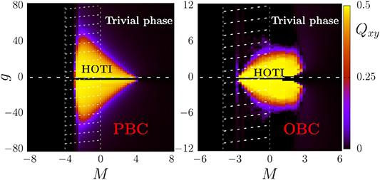
Figure 14. The phase diagram of the tight-binding model in equation (127) on amorphous lattices for a fixed scrambling radius  with respect to the parameters M and g, which is obtained by evaluating the quadrupole moment under periodic boundary conditions (left) and open boundary conditions (right). The HOTI phase in the crystalline system is marked by the white dashed region. Reproduced from [226]. CC BY 4.0.
Download figure:
Standard image High-resolution imageBased on the model (127), density-driven higher-order topological phase transitions are observed in [294]. Specifically, the authors map out the phase diagram in the  plane (ρ is the density of sites and M is the mass) based on the quadrupole moment qxy
(see figure 15(a)). The figure clearly illustrates that a system in a trivial phase at low density (e.g. ρ = 0.24) will become a nontrivial one at high density (e.g. ρ = 1). Figures 15(b) and (c) also illustrate that as the density increases, the bulk energy gap closes and reopens at the critical density ρ ≈ 0.41 and the quadrupole moment changes from 0 to 1, resulting in the corner modes.
plane (ρ is the density of sites and M is the mass) based on the quadrupole moment qxy
(see figure 15(a)). The figure clearly illustrates that a system in a trivial phase at low density (e.g. ρ = 0.24) will become a nontrivial one at high density (e.g. ρ = 1). Figures 15(b) and (c) also illustrate that as the density increases, the bulk energy gap closes and reopens at the critical density ρ ≈ 0.41 and the quadrupole moment changes from 0 to 1, resulting in the corner modes.

Figure 15. (a) The phase diagram of the tight-binding model in equation (127) on amorphous lattices with respect to the density ρ and the mass M, which is mapped out by the quadrupole moment qxy . (b) The energy spectrum under open boundary conditions (blue circles) and periodic boundary conditions (red circles) at M = 0. (c) The energy gap (red line for open boundaries and yellow line for periodic boundaries) and the quadrupole moment qxy (blue line) with respect to the density ρ at M = 0. (a)–(c) Reprinted figure with permission from [294], Copyright (2022) by the American Physical Society.
Download figure:
Standard image High-resolution imageRecently, the authors in [245] find that amorphous systems can support HOTPs without crystalline counterparts protected by an average Cp
T symmetry. For instance, the HOTIs can host eight or twelve corner modes, which cannot exist in crystalline systems. Specifically, they consider the Hamiltonian with  and
and

where p takes the value of a multiple of 4 and ![$f(|{\boldsymbol{d}}|) = \Theta(R-|{\boldsymbol{d}}|)\exp[-\lambda(|{\boldsymbol{d}}|/d_0-1)]/2$](https://content.cld.iop.org/journals/0953-8984/36/28/283002/revision2/cmad3abdieqn732.gif) . The lattice sites are positioned completely randomly with a hardcore radius
. The lattice sites are positioned completely randomly with a hardcore radius  in a regular p-gon. Although each configuration of lattice sites lacks p-fold rotation (Cp
) symmetry due to the randomness of site positions, the ensemble of sample configurations respects average Cp
symmetry. As a result, the ensemble of Hamiltonians respects average Cp
M and Cp
T symmetry, i.e.
in a regular p-gon. Although each configuration of lattice sites lacks p-fold rotation (Cp
) symmetry due to the randomness of site positions, the ensemble of sample configurations respects average Cp
symmetry. As a result, the ensemble of Hamiltonians respects average Cp
M and Cp
T symmetry, i.e.  , where
  ,
,  and
and  is the Hamiltonian on lattice configuration
  (see section 4.1.2 for detailed discussions on average symmetry).
To characterize the topological properties, the authors build a  topological invariant based on the
  symmetry by imposing twisted boundary conditions [245]. In addition, since the model has the chiral symmetry represented by
  , one may ask whether the topological phase can be characterized by the traditional quadrupole moment defined in equation (13). However, when directly evaluating the quadrupole moment, it consistently yields zero. This may be attributed to the presence of an even number of corner states in each quadrant within a nontrivial phase. To address this issue, the authors in [245] propose a solution whereby the positions of sites within a
  sector and its opposite counterpart are relocated to the first and third quadrants, respectively. Likewise, the sites in other sectors are relocated to the second and fourth quadrants, respectively (see figures 16(a) and (b) for an example of an octagon geometry with p = 8).

Figure 16. (a) and (b) Schematics of changing site positions in a regular octagon with p = 8 for correctly computing the quadrupole moment. The site positions in the orange (blue) region in (a) are transformed to the first or third (second or fourth) quadrant in (b). The quadrupole moment is calculated using the deformed lattices and the original eigenstates. (c) The configuration averaged  topological invariant
  (solid lines) and quadrupole moment
  (dotted lines) calculated from the reconstructed lattices of different sizes with respect to mz
for the amorphous HOTI model with the average
(dotted lines) calculated from the reconstructed lattices of different sizes with respect to mz
for the amorphous HOTI model with the average  symmetry. (d) The configuration averaged local DOS at zero energy in the amorphous HOTI phase on a regular octagon. (a)–(d) Reproduced from [245]. CC BY 4.0.
Download figure:
Standard image High-resolution imageThe authors evaluate the averaged  topological invariant
  and the quadrupole moment
  based on the transformed site positions, which correctly characterize the higher-order topological amorphous insulators in an octagon with p = 8, as shown in figure 16(c). The HOTI phase is further supported by the existence of corner modes indicated by the profile of local density of states (DOS) (see figure 16(d)). Moreover, the average symmetry protected HOTIs are found to exist in amorphous lattices of a dodecagon for p = 12 as well [245]. In addition, it is shown that the higher-order topology in 2D quasicrystalline lattices can also be characterized by the generalized quadrupole moment [246]. In 3Ds, the winding number of the generalized quadrupole moment and a
  invariant based on transformed site positions are defined to characterize the chiral and helical modes without crystalline counterparts [246] (see section 4.2 for a detailed discussion).
4.1.2. Three dimensions.
In sections 2.3 and 2.4, we present a chiral and helical model in 3D crystalline systems to show the existence of chiral and helical hinge modes. There, we see that the crystalline symmetry such as the  symmetry is required to protect the quantization of the Chern–Simons invariant, implying that the topological invariant is not well defined if we consider amorphous lattices, which break the symmetry. Fortunately, the winding number of the quadrupole moment is not dependent on any symmetry, making it possible to realize chiral hinge modes in amorphous lattices. Indeed, the authors in [137] predict the existence of SOTIs without TRS (see the hinge states in figure 17(a)) and with TRS in amorphous lattices and structural disorder induced second-order topological phase transition.

Figure 17. (a) The density distribution of four states near zero energy in the SOTI phase, exhibiting the hinge modes. (b) The quadrupole moment Qxy
with respect to the flux  , reflecting the nontrivial winding number of the quadrupole moment. (c) Sample averaged two-terminal conductance
  [blue (system size L = 30) and green lines (L = 40)] and winding number of the quadrupole moment
  [red line (L = 16)] of the 3D amorphous model as a function of the mass M. The black line describes the conductance of the Hamiltonian on a cubic lattice. (d) Sample averaged bulk energy gap (green and blue lines) of the 3D amorphous model with respect to M compared with the results (black line) on a cubic lattice The red line depicts the DOS at zero energy. (a)–(d) Reprinted figure with permission from [137], Copyright (2021) by the American Physical Society.
Download figure:
Standard image High-resolution image4.1.2.1. Amorphous SOTI.
The tight-binding Hamiltonian  studied in [137] includes the onsite mass term
  and the hopping matrix

from site
r
to  with
with  and
and ![$f(|{\boldsymbol{d}}|) = \Theta (R-|{\boldsymbol{d}}|)\exp[-\lambda(|{\boldsymbol{d}}|/d_0-1)]/2$](https://content.cld.iop.org/journals/0953-8984/36/28/283002/revision2/cmad3abdieqn764.gif) . For regular cubic lattices with only nearest-neighbor hoppings, the Hamiltonian reduces to the paradigmatic 3D SOTI model in equation (73). The SOTI phase is protected by the winding number of the quadrupole moment about the momentum kz
, which requires no spatial symmetry, and thus it is possible for SOTIs to persist in completely random lattice sites. In amorphous systems, there is no well-defined momentum kz
due to the lack of translational symmetry. Therefore, the authors insert a flux
. For regular cubic lattices with only nearest-neighbor hoppings, the Hamiltonian reduces to the paradigmatic 3D SOTI model in equation (73). The SOTI phase is protected by the winding number of the quadrupole moment about the momentum kz
, which requires no spatial symmetry, and thus it is possible for SOTIs to persist in completely random lattice sites. In amorphous systems, there is no well-defined momentum kz
due to the lack of translational symmetry. Therefore, the authors insert a flux  through a twisted the boundary condition along z in place of kz
and calculate the winding number of the quadrupole moment with respect to
through a twisted the boundary condition along z in place of kz
and calculate the winding number of the quadrupole moment with respect to  [137], defined as

where  is the quadrupole moment in the (x, y) plane, which is a function of the inserted flux
  . The flux can also be added by introducing a phase factor
  to the hopping term. In a SOTI phase, a nontrivial winding number of
  arises when one tunes
  from 0 to 2π, as illustrated in figure 17(b) for a disorder configuration.
The study finds the existence of a second-order topological region with almost quantized winding number of one and quantized two-terminal conductance of  along the z direction arising from chiral hinge states (see figure 17(c)).
In the presence of TRS, the authors construct a tight-binding Hamiltonian [137]

where  , the onsite mass term
  and the hopping matrix

with  denoting another set of Pauli matrices. The TRS represented by
  is respected, i.e.
  , where
  and
and  with
with  . On a cubic lattice, the Hamiltonian reduces to the model in equation (84) with an extra term proportional to
  .
.
When t3 = 0, the pseudospin sy
is a conservative quantity and the topological properties can be identified by the winding number of the spin quadrupole moment about a flux  ,
,

where  is the spin quadrupole moment as defined in section 2.4.2 but with the momentum kz
replaced by the flux
is the spin quadrupole moment as defined in section 2.4.2 but with the momentum kz
replaced by the flux  . As a result, the HOTP can be characterized by the spin winding number defined in equation (86). It is also shown that for small t3, the spin winding number is still applicable even though sy
is not a conservative quantity. Besides, a
. As a result, the HOTP can be characterized by the spin winding number defined in equation (86). It is also shown that for small t3, the spin winding number is still applicable even though sy
is not a conservative quantity. Besides, a  invariant is defined to characterize the topological phase [see equation (91) in section 2.4.2 for its definition. Here, the momentum kz
should be replaced by a flux
invariant is defined to characterize the topological phase [see equation (91) in section 2.4.2 for its definition. Here, the momentum kz
should be replaced by a flux  ].
].
Numerical calculations reveal a range of M with sample averaged  topological invariant
  and spin winding number
  quantized at 1 up to finite-size effects, as shown in figure 18(b), indicating the existence of an amorphous SOTI phase with TRS. The topological helical hinge states manifest in the two-terminal conductance quantized at
  .
.

Figure 18. (a) Structural disorder induced SOTI, illustrated by the sample averaged two-terminal conductance  (blue and green lines), winding number of the quadrupole moment
  (black line) and bulk energy gap (red line) of the 3D amorphous model without TRS with respect to the disorder strength W. (b) Sample averaged two-terminal conductance
  (blue line) and
  topological invariant (red line) of the 3D amorphous model with TRS as a function of M. The black and green lines describe the conductance and
  topological invariant of the model on a cubic lattice, respectively. (a) and (b) Reprinted figure with permission from [137], Copyright (2021) by the American Physical Society.
Download figure:
Standard image High-resolution image4.1.2.2. Structural disorder induced SOTI.
Structural disorder refers to position randomness of lattice sites, serving as a bridge between a crystalline system and an amorphous system. The authors in [137] also demonstrate that structural disorder can drive a topological phase transition from a trivial phase to a SOTI. The induced transition can be seen from the jump of the conductance and the winding number of the quadrupole moment from zero and the bulk energy gap closure as shown in figure 18(a). The driven SOTI also exhibits the hinge states as revealed by the local DOS.
4.1.2.3. Average symmetry protected bulk energy gap closure.
In figures 17(d) and 18(a), we see that the higher-order topological phase transition occurs both through the closure of the bulk energy gap, although the  symmetry is broken in each sample. Here, we will follow [137] to show that such a bulk energy gap closure happens due to the
  symmetry on average. One can also apply similar argument to the 2D case in section 3.1.
To demonstrate that the Hamiltonian  respects the average
  symmetry, one can calculate the symmetry counterpart of the Hamiltonian,


In the derivation, the results are used:  and
and  . We use S to represent a set of all site positions in a disorder sample and then rotate all site positions in S in a counterclockwise direction about z by 90 degrees to obtain a new set
  . If we consider cubic lattices, then
  so that
  , showing that the
  symmetry is obeyed. However, for a typical individual disorder configuration,
  , and we usually have
  , indicating that the symmetry is absent.
We now consider a statistical ensemble consisting of all systems. The ensemble is defined to respect an average symmetry if a Hamiltonian and its symmetry conjugate partner exist in the ensemble with the same probability [279, 280]. For instance, a configuration S and its rotational part  clearly appear with the same probability since we consider the structural disorder without any correlation. As a consequence, the probability of occurrence of
  is equal to that of its
  conjugate partner
  so that the ensemble respects the
  symmetry on average.
We now argue that this average symmetry enforces the bulk energy gap closure at the phase transition point for a single system [137]. To demonstrate it, we consider a subsystem  whose z coordinates are restricted in the interval
 ![$[z_0,z_0+\Delta z]$](https://content.cld.iop.org/journals/0953-8984/36/28/283002/revision2/cmad3abdieqn809.gif) inside a large system (see figure 19). As a single system with a spatial configuration S1, the subsystem does not respect the
inside a large system (see figure 19). As a single system with a spatial configuration S1, the subsystem does not respect the  symmetry so that the topological phase transition happens through a surface energy gap closing, e.g. the energy gap on the x-normal surface. For a very large system (e.g. infinitely long along z), it is reasonable to expect that there exists the spatial configuration
  , which is obtained by rotating S1 about z by 90 degrees and shifting the coordinate along z by α. This leads to another subsystem
  with the spatial configuration S2 (see figure 19). It is clear to see that
  is the
  conjugate partner of
  . Therefore, when the x-normal surface energy gap of
  vanishes, the y-normal surface energy gap of
  must close. It indicates that for the entire system including both
  and
and  , the closure of the energy gap must simultaneously occur on both surfaces, suggesting that the bulk energy gap should close.

Figure 19. Schematic illustration of a system including two subsystems  and
and  on the site configurations of S1 and S2, respectively. Reprinted figure with permission from [137], Copyright (2021) by the American Physical Society.
Download figure:
Standard image High-resolution image4.2. Quasicrystalline lattices
Another class of non-crystalline materials is quasicrystals which lack translational symmetry while possess quasi long-range order [150]. Quasicrystals can also respect five-fold, eight-fold, ten-fold or twelve-fold rotational symmetry, which are not allowed in crystalline systems. These symmetries enable the existence of new HOTPs in both 2Ds [228–237] and 3Ds [246, 295], which cannot appear in crystalline systems.
Higher-order topological superconductors with Majorana zero modes localized at eight corners of an octagonal sample can occur on a 2D Ammann–Beenker (AB) tiling quasicrystalline lattice with eight-fold rotational symmetry (see figure 20) [228]. The authors consider the following mean-field real-space many-body Hamiltonian on a AB tiling quasicrystalline lattice,

where  with
with  (
( ) creating (annihilating) an electron with spin ν at site j, the mass term
  , and the hopping matrix

where Δ is the p-wave pairing strength, θjl
is the polar angle between site j and l, and  denotes a pair of sites connected by an edge on the lattice. This Hamiltonian can be written as
  where HBdG is the Bogoliubov-de-Gennes (BdG) Hamiltonian and
  . The system respects the particle-hole symmetry, i.e.
  where
where  , and the chiral symmetry, i.e.
  with
with  (I is an identity matrix acting on the degrees of freedom of lattice sites).

Figure 20. The spatial distributions of the corner modes of the higher-order topological superconductor on an AB tiling quasicrystal sample. Reprinted figure with permission from [228], Copyright (2019) by the American Physical Society.
Download figure:
Standard image High-resolution imageWhen V = 0, HBdG is a model consisting of two Chern bands with opposite Chern number, thereby contributing helical Majorana edge modes. In fact, the helical edge modes are protected by a time-reversal like symmetry represented by  . The V term breaks the symmetry and gaps out the edge states by introducing an effective mass on each surface; such masses change sign across each neighboring edges, giving rise to Majorana corner modes, as discussed in section 2.1.2. While the V term also breaks the C8 symmetry, the
  symmetry is preserved with
  [228].
To define a topological invariant, the authors in [228] construct an effective Hamiltonian  , where

with  being the zero-energy Green's function and
  being the plane-wave state with momentum k. Here, n labels the local components composed of spin and particle-hole degrees of freedom. The plane-wave state is defined on a four-dimensional (4D) cubic lattice which generates the 2D quasicrystal through the cut-and-project method [228]. Since the system respects the
  symmetry, one can restrict Heff at the C8-invariant momenta
  and
and  to the eigenspace of
  with eigenvalues
  (
( ). At each subspace, the restricted Hamiltonian still respects the particle-hole symmetry and thus is classified as the zero-dimensional class D. One thus can calculate the sign (denoted by
  ) of the Pfaffian of an antisymmetric Hamiltonian transformed from the original Hamiltonian. A
  invariant is thus defined as

where  . It is found that in the nontrivial phase with corner modes,
  whereas in the trivial one, ν = 1.
HOTIs can also arise in quasicrystals [229]. The authors in [229] study a model Hamiltonian with the onsite term  and the hopping matrix

on an AB tiling quasicrystal where  describes the decay of the hopping with respect to the distance d between two sites. Similarly, when g = 0, the Hamiltonian describes a quantum spin Hall insulator protected by TRS represented by
  and conserved spin σz
[229], hosting helical edge modes. The g term breaks the TRS so as to open an energy gap at boundaries. With this term, the system still respects the particle-hole symmetry represented by
and conserved spin σz
[229], hosting helical edge modes. The g term breaks the TRS so as to open an energy gap at boundaries. With this term, the system still respects the particle-hole symmetry represented by  and chiral symmetry represented by
  .
.
Approximately, the effective mass at each edge depends on  where θedge is the polar angle of a boundary. For η = 2, the mass's sign is positive for
 ![$\theta_{\textrm{edge} }\in [-\pi/4,\pi/4]\cup [3\pi/4,5\pi/4]$](https://content.cld.iop.org/journals/0953-8984/36/28/283002/revision2/cmad3abdieqn855.gif) (labeled by red color) while it becomes negative for
(labeled by red color) while it becomes negative for ![$\theta_{\textrm{edge} }\in [-3\pi/4,-\pi/4]\cup [\pi/4,3\pi/4]$](https://content.cld.iop.org/journals/0953-8984/36/28/283002/revision2/cmad3abdieqn856.gif) (labeled by blue color), as shown in figures 21(a) and (b). For a quasicrystal lattice with pentagon boundaries, shown in figures 21(a), (e) and (i), there appear four zero-energy states localized at corners where the mass exhibits a sign change. For an octagon, the masses are zero at four edges while the sign of the mass at its two neighboring edges is opposite, leading to edge states extended along the four edges (see figures 21(b) and (j)). In fact, these edge states can be understood as corner states as one can continuously deform the boundary into a vertex so that a square is formed and corner states are localized at the corners. Similarly, when η = 4, the system exhibits eight-fold symmetric zero-energy corner states for octagon boundaries (see figure 21(k)) and for pentagon boundaries, only two corner states appear (see figure 21(l)). The HOTI can be characterized by the
(labeled by blue color), as shown in figures 21(a) and (b). For a quasicrystal lattice with pentagon boundaries, shown in figures 21(a), (e) and (i), there appear four zero-energy states localized at corners where the mass exhibits a sign change. For an octagon, the masses are zero at four edges while the sign of the mass at its two neighboring edges is opposite, leading to edge states extended along the four edges (see figures 21(b) and (j)). In fact, these edge states can be understood as corner states as one can continuously deform the boundary into a vertex so that a square is formed and corner states are localized at the corners. Similarly, when η = 4, the system exhibits eight-fold symmetric zero-energy corner states for octagon boundaries (see figure 21(k)) and for pentagon boundaries, only two corner states appear (see figure 21(l)). The HOTI can be characterized by the  topological invariant ν [228].

Figure 21. (a)–(d) Illustrations of the angle dependence of the sign of the effective masses near a corner of pentagonal and octagonal AB tiling quasicrystal samples. The red and blue color represents the effective mass with opposite signs. (e)–(h) The energy spectrum under open boundary conditions. (i)–(l) The corresponding real-space distributions of zero-energy states. For the first and second columns, η = 2 and for the third and fourth columns, η = 4. (a)–(d) Reprinted figure with permission from [229], Copyright (2020) by the American Physical Society.
Download figure:
Standard image High-resolution imageThe authors in [229] also construct a Hamiltonian on the AB tiling quasicrystalline lattice with the onsite term  and the hopping matrix

where  and
and  with
with  . The system also has chiral symmetry represented by τ3 and thus the quadrupole moment qxy
is a quantized quantity [134, 135]. Indeed, it is found that in the nontrivial phase
. The system also has chiral symmetry represented by τ3 and thus the quadrupole moment qxy
is a quantized quantity [134, 135]. Indeed, it is found that in the nontrivial phase  , and four zero-energy corner states emerge in a geometry with square boundaries [229]. However, for the case with eight or more corner states, this quadrupole moment vanishes, and one needs to calculate the generalized quadurpole moment based on transformed lattice sites [245, 246].
We have shown that an even number of corner modes can exist in a quasicrystalline lattice. One may wonder whether five corner modes can appear in a Penrose tiling quasicrystalline lattice as the lattice has the five-fold rotational symmetry. Since the sign change of the mass can only give rise to even number of corner modes, one may consider other mechanisms. Indeed, the authors in [232, 234] find that a Penrose tiling quasicrystal can support five corner modes associated with a fractional charge  as shown in figure 22(a). To generate the corner modes, they apply an in-plane Zeeman field to a TI with helical edge states on a quasicrystal to gap out the edge states, leading to an effective Hamiltonian at a boundary

where  with ζj
being the orientation angle of the jth edge (see figure 22(b)), k1 is the momentum along the edge, θ is the polar angle of the Zeeman field. It has been shown that even though a mass kink Δζ across neighboring boundaries does not lead to the sign change of the mass, it can still result in a corner state associated with a fractional charge of
with ζj
being the orientation angle of the jth edge (see figure 22(b)), k1 is the momentum along the edge, θ is the polar angle of the Zeeman field. It has been shown that even though a mass kink Δζ across neighboring boundaries does not lead to the sign change of the mass, it can still result in a corner state associated with a fractional charge of  [296–298]. It is found that for a pentagonal Penrose tiling quasicrystal, five corner modes appear associated with a fractional charge
  due to the angle change of adjacent edges
  [234].

Figure 22. (a) The energy spectrum of a pentagonal Penrose tiling quasicrystal sample subject to an in-plane Zeeman field, exhibiting five corner modes at the energy EF . The inset displays the spatial distribution of the corner states. (b) Schematic illustration of an edge whose polar angle measured relative to the positive x axis is ζ. (a) and (b) Reprinted figure with permission from [234], Copyright (2022) by the American Physical Society.
Download figure:
Standard image High-resolution imageWhile the HOTIs in 2D quasicrystals indicate the existence of new TIs without crystalline counterparts, it remains unclear whether novel chiral and helical HOTIs without crystalline counterparts can occur in 3Ds. Very recently, the authors in [246] construct a 3D model by stacking 2D models on the AB tiling quasicrystalline lattices and find the existence of eight gapless chiral hinge modes, leading to the two-terminal conductance of  . The TI is characterized by the winding number of the generalized quadrupole moment based on transformed lattice sites. In the presence of TRS, it is shown that eight helical pairs of hinge modes arise, resulting in the conductance of
  . The phase is characterized by a
  topological invariant as well as the spin winding number of the quadrupole moment based on transformed lattice sites. In addition, higher-order Weyl-like and Dirac-like semimetals in quasicrystals supporting both surface Fermi arcs and hinge Fermi arcs have been theoretically predicted [246, 295].
4.3. Hyperbolic lattices
Recently, there has been a surge of interest in hyperbolic lattices [220–222, 225, 299–314], which belong to the category of 2D non-crystalline lattices. Compared with a crystalline system, any rotational symmetry is allowed in a hyperbolic lattice, providing another platform to realize HOTPs without crystalline counterparts. The arbitrary rotational symmetry comes from the fact that a hyperbolic lattice with constant negative curvature can be tessellated by regular p-gons with any integer p. The hyperbolic lattice in fact respects the hyperbolic translational symmetry. In other words, the lattice can be obtained by applying translational operations to the first unit cell on the hyperbolic plane. For example, in the hyperbolic {8,3} lattice, the translational operators are generated by four generators  and γ4 (see figure 23(a)). These translational operations form a non-Abelian group. One can also project the hyperbolic lattice onto a Poincar
 disk as shown in figure 23. Since the lattice sites on the disk break the traditional translational symmetry, we classify them as non-crystalline lattices.

Figure 23. (a) Schematic illustration of the {8,3} hyperbolic lattice projected onto the Poincar disk. (b) The {8,3} hyperbolic lattice on the Poincar
 disk with the first unit cell enclosed by the green curve and
  and γ4 representing four translational operators. The corner states are highlighted by yellow circles.
(a) and (b) Reprinted figure with permission from [238], Copyright (2023) by the American Physical Society.
and γ4 representing four translational operators. The corner states are highlighted by yellow circles.
(a) and (b) Reprinted figure with permission from [238], Copyright (2023) by the American Physical Society.
Download figure:
Standard image High-resolution imageIt is found that hyperbolic lattices can also give rise to HOTPs without crystalline counterparts due to the rotational symmetry absent in crystalline systems [238, 239]. Here, we follow [238] to present how the new phases arise. The authors construct two tight-binding models. For the first model, the Hamiltonian within the first unit cell reads

where  represents the creation operator for the αth orbital at site i in the rth unit cell on a hyperbolic lattice, and
  is given by equation (130). The hopping between sites in the first unit cell and sites in neighboring unit cells (the set S1) is given by

with modified polar angle  . The entire Hamiltonian can be derived through the application of hyperbolic translational operations, ensuring that it respects the hyperbolic translational symmetry.
The momentum-space Hamiltonian  in a 4D Brillouin zone with
 ![$k_j\in [0,2\pi]$](https://content.cld.iop.org/journals/0953-8984/36/28/283002/revision2/cmad3abdieqn881.gif) (
( ) is constructed based on the hyperbolic band theory [225]. One can keep two momenta
  out of the 4D momentum space
  as parameters and apply the Fourier transformation to the other two momenta, yielding a real-space Hamiltonian on a square lattice. In this way, the quadrupole moment
  can be calculated and the averaged quadrupole moment over
  is defined as
  . It is proved that
  and
and  due to the
  symmetry. It is found that the average quadrupole moment
  is quantized to 0.5 when g is not very large, suggesting the existence of HOTP. However, the real-space calculations do not suggest the existence of robust corner modes as the energy spectrum differs significantly for distinct system sizes.
We note that the authors in [314] calculate the bulk DOS in the BBH model on a  hyperbolic lattice that preserves the hyperbolic translational symmetry by a supercell method and find that the DOS exhibits a gap closing at a critical point. However, the bulk-edge correspondence has not been explored.
To find a higher-order phase, the requirement of the hyperbolic translational symmetry is relaxed and the following Hamiltonian on the hyperbolic lattice is studied [238],

where  represents the creation operator for the αth orbital at site i. This system exhibits zero-energy modes in the energy spectrum for a hyperbolic lattice under open boundary conditions (see figure 24(a)). The topological properties are characterized by the corner charge which approaches the quantized value of 0.5. Interestingly, in contrast to the quasicrystal case, there are two energy gaps: the minigap determined by the first nonzero eigenenergy and the edge energy gap determined by the energy where the degeneracy suddenly changes from the eight-fold to the double one (see figure 24(b)). Inside the edge gap, there are infinite number of eight-fold degenerate corner modes besides the zero-energy ones (see the spatial distribution of the states in figure 24(c)). Although the minigap may decrease to zero in the thermodynamic limit, finite-size analysis suggests that the zero-energy corner modes persist. In addition, HOTIs with 12, 16 or 20 corner modes have been found as shown in figures 24(d)–(f).

Figure 24. (a) The energy spectrum of the Hamiltonian in equation (147) with respect to the system parameter g on a hyperbolic {8,3} lattice at epoch 5 with 2888 sites, illustrating the presence of the zero-energy states. (b) The eigenenergies when g = 0.6 at epoch 6. The minigap represents the first nonzero positive energy and the edge gap represents the energy where the degeneracy suddenly changes from the eight-fold to the double one. Inside the edge gap, all states are eight-fold degenerate. (c) The spatial distributions of the wave functions in the vicinity of zero energy over the 1/8 sector on the boundary of the Poincar disk, suggesting that the eight-fold degenerate states are spatially localized around a corner while the states whose energy is slightly above the edge gap are more like the edge state. The zero-energy local DOS of hyperbolic (d) {12, 3} lattice, (e) {16, 3} lattice and (f) {20, 3} lattice.
(a)–(f) Reprinted figure with permission from [238], Copyright (2023) by the American Physical Society.
disk, suggesting that the eight-fold degenerate states are spatially localized around a corner while the states whose energy is slightly above the edge gap are more like the edge state. The zero-energy local DOS of hyperbolic (d) {12, 3} lattice, (e) {16, 3} lattice and (f) {20, 3} lattice.
(a)–(f) Reprinted figure with permission from [238], Copyright (2023) by the American Physical Society.
Download figure:
Standard image High-resolution image4.4. Fractal lattices
Fractals are another class of non-crystalline systems with detailed structure at arbitrarily small scale [223]. The fine structure at small scale is the same as or reminiscent of the whole pattern, which is the so-called self-similarity property. Usually a fractal lattice can be generated recursively. Figure 25 shows two well-known examples of fractals, Sierpiński triangle and von Koch curve. Another salient feature of fractals is the non-integer dimension. For the Sierpiński triangle, if each line segment is enlarged 2 times, we will get 3 copies of itself, giving the Hausdorff dimension  . Similarly, the dimension of the von Koch curve is
  . Note that there exist different definitions of dimensions in the context of fractals [223].

Figure 25. Two famous examples of fractals, (a) Sierpiński triangle and (b) von Koch curve. [223] John Wiley & Sons. © 2003 John Wiley & Sons, Ltd.
Download figure:
Standard image High-resolution imageRecently, it has been demonstrated that fractal lattices can also harbor HOTPs [213, 224, 240–244]. In [240], the authors study a Hamiltonian in equation (127) on a square Sierpiński carpet fractal with  and
and

As we have discussed previously, the Hamiltonian describes a quantum spin Hall insulator with the edge states gapped by a mass term. The energy spectrum exhibits in-gap corner states, as shown in figures 26(a) and (b). The four zero-energy states denoted by red dots in the inset of figure 26(a) are localized at the outer corners (see the upper panel of figure 26(b)) and the four states near zero energy colored blue in the inset of figure 26(a) are localized around the inner corners (see the lower panel of figure 26(b)). Note that the peaks of the local DOS of the inner corner states are not located at the exact inner corner sites (see the lower panel of figure 26(b)), which might be because the coordination number of these sites is larger than 2. The higher-order topological nature of the system is further illuminated by the quantized quadrupole moment  calculated under open boundary conditions, which is independent of the origin choice in the thermodynamic limit. The phase diagram is shown in figure 26(c) [240]. The authors of [240] also study the same Hamiltonian on a glued Sierpiński triangle fractal, which exhibits zero-energy states located at both the inner and outer corners (see figure 26(d)). The number of zero-energy modes can be large and rely on the generation number of the fractal lattice, while for a specific generation number, the number of corner states is the same under periodic and open boundary conditions. The higher-order topological nature of the model on the glued Sierpiński triangle fractal is also characterized by the quadrupole moment
  [240]. Besides HOTIs, higher-order topological superconductors can also reside on fractal lattices [240].

Figure 26. (a) The energy spectrum of the model on the square Sierpiński carpet fractal. The inset displays the zoom-in view of the states near zero energy. (b) Upper panel: local DOS of the four zero-energy states colored red in the inset of (a) which are localized at outer corners. Lower panel: local DOS of the four states near zero energy colored blue in the inset of (a). (c) The phase diagram of the model on the square Sierpiński carpet fractal in the  plane. (d) The local DOS of the zero-energy states of the model on the glued Sierpiński triangle fractal. (a)–(d) Reprinted figure with permission from [240], Copyright (2022) by the American Physical Society.
Download figure:
Standard image High-resolution image5. Experimental progress
In this section, we briefly summarize the progress in experimental realizations of HOTPs for both crystalline and non-crystalline systems.
5.1. Solid state materials
HOTPs in both 2Ds [57, 58, 61, 316–345] and 3Ds [38, 56, 64, 113, 346–349] have been predicted to exist in a bunch of solid state materials. Several classes of materials host multiple candidates for HOTIs in 2Ds, including hexagonal group-IV hydrides and halides (XY material with X = C, Si, Ge, Sn and Y = H, F, Cl) [328], hexagonal group-V materials (P, As and Sb) [316, 319, 324, 328, 336], Kekulé and anti-Kekulé group-IV materials (C, Si, Ge, Sn) [328], ferroelectric materials (e.g. In2Se3) [341], group-VIB transition metal dichalcogenides (MX2 material with M = W, Mo and X = Te, Se, S) [327, 337] and carbon allotrope with C≡C bond (graphyne and graphdiyne) [58, 61, 317, 320]. Other typical proposals for non-magnetic 2D HOTIs include twisted bilayer graphene and boron nitride for a range of twist angles [57, 321], antidot Dirac materials [323], semiconductor quantum wells [325] and so on. There are also many theoretical predictions of magnetic 2D HOTIs, such as bismuth on EuO substrate [318], NpSb [326], CrSiTe3 [343], 2H-RuCl2 [335], Janus VSSe [335] and CoBr2/Pt2HgSe3/CoBr2 van der Waals heterostructure [330]. FeSe is a possible HOTI with antiferromagnetic order [332, 334]. Besides electronic 2D HOTIs, the phononic conterparts are also predicted in C3N [344], graphyne [340] and graphdiyne [338]. Most recently, the authors of [345] propose TiSiCO family monolayers as a new class of 2D HOTIs for which the corner degree of freedom can be controlled by electric and optical fields and might have potential applications in novel electronic devices. For 3D materials, EuIn2As2 [56] and Bi Smx
Se3 [346] are predicted to be HOTIs with chiral hinge states. Antiperovskites such as Ca3SnO and Ca3PbO [347], distorted SnTe [38], MoTe2 [113], WTe2 [113] and La apatite [348] are possibly 3D HOTIs carrying helical hinge states. Besides, MnBi
Smx
Se3 [346] are predicted to be HOTIs with chiral hinge states. Antiperovskites such as Ca3SnO and Ca3PbO [347], distorted SnTe [38], MoTe2 [113], WTe2 [113] and La apatite [348] are possibly 3D HOTIs carrying helical hinge states. Besides, MnBi Te
Te is predicted to be a 3D higher-order Möbius insulator [64] and β-CuI is a candidate for higher-order Dirac semimetals [349].
For experimental aspects, HOTPs have only been found in a few solid state materials. Second-order topological corner modes in 2D fractal lattices have been observed in Bi monolayer deposited on InSb substrate recently [224]. Bulk bismuth (Bi) [350, 351], bismuth bromide (Bi4Br4) [315, 352] and layered Td -WTe2 [353–356] are experimentally denonstrated to have time-reversal symmetric 3D higher-order topology with 1D helical hinge states. The higher-order topology of bismuth are protected by the C3 and inversion symmetry and Bi4Br4 are protected by the C2 symmetry. Td -WTe2 is noncentrosymmetric and hosts nonsymmetry-indicated higher-order topology [113]. Among them, bulk Td -WTe2 (WTe2 in the orthorhombic structure) has been identified as a type-II Weyl semimetal in previous studies [357, 358] (note that type-II Weyl points are also called structured Weyl points [359]), bismuth is also metallic [350], and only Bi4Br4 is a gapped insulator [315]. Figure 27 displays the calculated bulk band structures of Bi4Br4 and bismuth. Bi4Br4 is an insulator with a bulk gap (see figure 27(a)). Its higher-order topology gives rise to gapless hinge states in the band spectrum of a Bi4Br4 nanowire (see figure 27(b)). As a comparison, bismuth is not an insulator since the energy bands have electron and hole pockets at the Fermi energy (see figure 27(c)). Nevertheless, the valence bands and conduction bands are separable by a direct gap across the Brillouin zone. Therefore, we can still define the bulk topological indices from the symmetry eigenvalues of the valence bands, corresponding to helical hinge states traversing the bulk gap in the spectrum for a nanowire of bismuth [350].

Figure 27. (a) The band structure for Bi4Br4 without (left) and with (right) spin–orbit coupling (SOC). There is a nonzero gap separating the conduction bands and valence bands. (b) The energy bands calculated for a nanowire of Bi4Br4, which exhibit the gapless hinge states crossing at a Dirac point. From [315]. (c) The band structure of bismuth. There is no gap at the Fermi energy denoted by the dashed line. (a)–(c) Reproduced from [315], with permission from Springer Nature.
Download figure:
Standard image High-resolution image
The hinge states can be observed directly by scanning tunnelling microscopy [350–352] and angle-resolved photoemission spectroscopy [315] and their transport properties can be measured by Josephson interferometry [350, 353–355]. The spin polarization of the helical hinge states is resolved by the magneto-optic Kerr-rotation measurement in Td -WTe2 [356]. Helical hinge states are also observed in Cd3As2 by Josephson interferometry measurements [360], consistent with the hinge Fermi arc calculated theoretically [121], implying Cd3As2 is a higher-order topological semimetal. Spin-momentum locking of the hinge states is evidenced by spin transport measurements [361]. There is also evidence that FeTe0.55Se0.45 might be a higher-order topological superconductor with helical hinge zero modes [362].
5.2. Synthetic systems
In addition to solid state materials, HOTPs are also realized in quantum simulators. An electronic SOTI in 2Ds is realized by manipulating carbon monoxide molecules as a breathing kagome lattice on Cu surface [363]. The 2D HOTI is also simulated by a superconducting qubit [364]. Much richer HOTPs are observed in a variety of metamaterials, such as mechanical [365–374], microwave [375], acoustic [131, 241, 242, 376–418], photonic systems [419–455], thermal metamaterials [456] and electric circuits [149, 457–465], blessed by their high tunability. HOTIs with corner states have been extensively simulated in various systems in both 2Ds [365–378, 380, 382, 383, 387, 391–393, 397–399, 408, 409, 411, 413–439, 441, 443, 444, 446, 451–455, 457, 459, 461, 463–465] and 3Ds [379, 384, 386, 389, 403–405, 412, 458, 460, 463]. In 3Ds, SOTIs with chiral [385], helical [406, 412] and zero-energy hinge states [410], higher-order Klein bottle TIs [131], second-order topological semimetals [395, 396, 402, 445], and HOTIs with surface, hinge and corner states coexisting in the same band gap [381, 383, 388, 390, 400] have also been realized in acoustic [381, 383, 385, 388, 390, 395, 400, 402, 406, 410, 412, 448, 449] and photonic systems [445]. Nonlinear second-order topological corner states in 2Ds are observed in photonic systems [440, 442] and Floquet SOTIs are investigated experimentally in an acoustic lattice [407]. By introducing synthetic dimensions, HOTPs in higher dimensions are realized in photonic and acoustic crystals [394, 401, 447]. The phase transition from an anomalous quantum Hall insulator to SOTIs induced by disorder is demonstrated experimentally in electric circuits [149]. Non-0D corner states are observed in acoustic fractal lattices [241, 242] and photonic quasicrystals with six-fold rotational symmetry [450]. Quadrupole TIs on quasicrystalline lattices have also been experimentally realized in electric circuits [462]. However, there, quasicrystal sites are arranged in a square sample and only four corner modes are observed. Despite the theoretical predictions of HOTIs in quasicrystals with five, eight, ten or twelve corner modes [228–234], which cannot exist in crystalline systems, their implementation poses a significant challenge for experiments. The challenge arises from the complex form of the Hamiltonian, which involves long-range hopping for metamaterial simulations.
6. Summary and perspectives
In this review, we have introduced the recent progress on HOTPs in both crystalline and non-crystalline systems. Different from conventional first-order topological phases, the HOTPs are featured by the topological boundary states of lower dimension. We review several prototypical examples of HOTPs including 2D quadrupole TIs, 3D SOTIs with either chiral or helical hinge states, and higher-order topological semimetals with hinge Fermi arcs, and introduce their topological boundary states and corresponding topological invariant. It has been demonstrated that some HOTIs are protected by the topological invariants which do not require the presence of crystalline symmetries. Therefore, these HOTPs can exist in disordered systems or non-crystalline systems that break crystalline symmetries. Then, we turn to discuss the HOTPs in the presence of quenched disorder. Similar to first-order topological phases, it has been shown that HOTPs are robust to weak disorder. We further demonstrate that disorder can induce a HOTI from a trivial insulator, which is the generalization of topological Anderson insulator to the higher-order case. On the other hand, structural disorder in irregular lattices can also have effects on HOTPs. It has been found that there exist SOTIs with chiral or helical hinge states in amorphous systems and structural disorder can remarkably drive a topological phase transition between a trivial insulator and a SOTI. In addition, we review the progress on HOTPs in other non-crystalline systems such as quasicrystals, hyperbolic lattices, and fractal lattices, which can host HOTPs beyond crystalline systems.
We remark that this review has only discussed a few models for HOTPs and many other aspects of higher-order topology have not been covered here. In addition to static systems, the HOTPs in nonequilibrium systems have also been extensively investigated. In [67, 364, 466–472], people have studied the far-from-equilibrium dynamics of various HOTPs after a sudden quench of the Hamiltonian. Interestingly, the authors in [67] found that a quadrupole TI after the quench will undergo a topological transition from a trivial phase to a quadrupole topological insulating phase during the unitary time evolution. On the other hand, a number of works studied the Floquet higher-order topology in periodically driven systems [466, 473–493]. Similarly to the first-order cases, people discovered the Floquet HOTPs with anomalous corner or hinge modes and the corresponding topological invariants were also proposed [492]. In the review, we have focused on the HOTPs for noninteracting fermions, which can be effectively described by topological band theory. Several works have studied higher-order symmetry-protected topological phases in interacting fermion or boson systems which exhibit gapless corner or hinge modes [494–511]. Besides HOTIs and semimetals we have discussed, higher-order topological superconductors have also gained much attention for the Majorana modes at corners or hinges, which provide alternative platforms to realize non-Abelian braiding for topological quantum computation in the future [512–518].
So far, most studies have been focused on HOTPs at zero temperature, while only a few of works have covered HOTPs at finite temperature. For a topological insulator of noninteracting fermions, the system is in a many-body ground state that all particles occupy the bands below the gap at zero temperature. At finite temperatures, the system in thermal equilibrium is described by a mixed state rather than a single ground state. In recent years, people have developed concepts and characterizations for the first-order TIs at finite temperatures, including the topological invariant for ensembles [519–524]. One immediate problem worth studying is generalizing the formalism to HOTPs. Another interesting problem is about higher-order topology tuned by the temperature. At finite temperatures, thermal fluctuations play a similar role as disorder which can drive phase transitions [524]. On the other hand, various symmetry-breaking orders such as superconducting pairings or magnetizations may have dependence on the temperature, which can affect the bulk topology at mean-field level accordingly. In [98], the authors studied a 2D extended Hubbard model with spin–orbit coupling and found that the temperature can drive a phase transition between a gapped second-order topological superconductor and a gapless superconductor, which results from the change of favored pairing type at a critical temperature.
On the topological characterization of HOTIs, there exists an open question about the properties of the quadrupole moment as a topological invariant. It has been found that the quadrupole moment can change when either the bulk energy gap or edge energy gap closes while the quantity itself is evaluated from the bulk wave functions without boundaries. Moreover, the current operator-based definition of the quadrupole moment may have some inconsistent results for some cases as pointed out in [250]. Another problem worth studying is about HOTPs in a system with gauge flux leading to momentum-space nonsymmorphic symmetry [525]. Recently, multipole TIs with corner modes and HOTIs with hinge modes have been found in lattice models respecting the glide-reflection symmetry in momentum space [76, 77, 131]. The momentum-space nonsymmorphic symmetries may enrich the family of HOTPs.
Acknowledgments
We appreciate the collaboration with L-M Duan, G Chen, S A Yang, Q-B Zeng, Y-L Tao, Y-F Mao, N Dai and M Yan on the topic. We thank B Wieder, R-J Slager and S Zhang for helpful discussions. This work is supported by the National Natural Science Foundation of China (Grant No. 11974201) and Tsinghua University Dushi Program and Innovation Program for Quantum Science and Technology (Grant No. 2021ZD0301604). We also acknowledge the support by center of high performance computing, Tsinghua University.
Data availability statement
The paper is a review article which does not contain original data. The data that support the findings of this study are available upon reasonable request from the authors.