
Abstract
We calculate the linear and the second harmonic (SH) spin current response of two anisotropic systems with spin–orbit (SO) interaction. General expressions of wide applicability for the these response functions are first derived for a generic two-band Hamiltonian. The first system is a two-dimensional (2D) electron gas in the presence of Rashba and k-linear Dresselhaus SO couplings. The calculations show how narrow or wide the response spectra can be, what is their overall shape and size, and frequency shiftings, depending on which crystal orientation is selected. The quantitative knowing of this makes possible a comparative study for several orientations, which would allow to select a spectrum with particular characteristic. We find that vanishing linear and second order response tensors are achievable under SU(2) symmetry conditions, characterized by a collinear SO vector field. Additional conditions under which specific tensor components vanish are possible, without having such collinearity. Thus, a proper choice of the growth direction and SO strengths allows to select the polarization of the linear and SH spin currents according to the direction of flowing. The second system is an anisotropic 2D free electron gas with anisotropic Rashba interaction, which has been employed to study the optical conductivity of 2D puckered structures with anisotropic energy bands. The presence of mass anisotropy and an energy gap open several distinct scenarios for the allowed optical interband transitions, which manifest in the linear and SH response contrastingly. The linear response displays only out-of-plane spin polarized currents, while the SH spin currents flow with spin orientation lying parallel to the plane of the system strictly. The models illustrate the possibility of the nonlinear spin Hall effect in systems with SO interaction, under the presence or absence of time-reversal symmetry. The results suggest different ways to manipulate the linear and nonlinear optical generation of spin currents which could find spintronic applications.
Export citation and abstract BibTeX RIS

Original content from this work may be used under the terms of the Creative Commons Attribution 4.0 license. Any further distribution of this work must maintain attribution to the author(s) and the title of the work, journal citation and DOI.
1. Introduction
The two-dimensional electron gas (2DEG) in semiconductor heterostructures has maintained its relevance even after almost two decades of constant discovery of new 2D materials. Even before graphene [1], these quantum wells were the subject of constant research due to their potential applications in the field of spintronics that the presence of spin-orbit (SO) coupling provides [2, 3]. The spin Hall effect [4, 5], the current-induced spin polarization [6], a nonballistic version of a spin transistor [7, 8], and the persistent spin helix state [9] are remarkable examples of spin-dependent phenomena associated to the SO interaction in 2DEGs. The art of manipulating spin using SO coupling gave birth to the field called spin-orbitronics, also dubbed 'Rashba-like physics' [10–12], inspired by the Rashba SO coupling, which leads to spin-momentum locking in low dimensional systems lacking inversion symmetry [3]. This new field involves the study of spin currents, its generation, transport, and detection. Recently, the investigation has been extended to explore the nonlinear spin current response as an alternative mechanism of generation. Spin and valley currents to the second order in the electric fields were predicted for 2D crystals like graphene, monolayer and trilayer transition-metal dichalcogenides, and monolayer GaSe [13]. The optical generation of dc spin currents by second-order nonlinear interactions in 2DEGs with SO coupling has also been explored [14–16].
One of the most studied 2DEG systems is the one that includes the Rashba and the linear Dresselhaus SO contributions. The interplay between these couplings leads to an anisotropic spin-splitting responsible of effects like a characteristic frequency dependence of the charge and spin Hall conductivities [17], the anisotropy of plasmon dynamics [18], or persistent spin textures [19–21], among others. It also allows the possibility of spin-preserving symmetries and associated effects like the infinite spin lifetime due to fixed spin precession axis [20], the mentioned nonballistic spin field-effect transistor [7], the suppression of spin beats in oscillations of magnetoresistivity [22], the vanishing of Zitterbewegung [23, 24], the vanishing of the interband absorption and spin Hall conductivity [25], or the cancelation of plasmon damping [18], all with potential device applications. Despite the extensive research, the investigation has usually been restricted to quantum wells grown along the [001], [110], or [111] direction [7, 14, 19, 20, 26–40]. With respect to growth along low-symmetry crystal orientations, there are some experiments reported. Ganichev and Golub in [41] used photogalvanic spectroscopy to probe Rashba + Dresselhaus spin splittings in quantum wells assembled on heterostructures oriented along the [001], [111], [110], [113], [112], and [013] directions, and address the requirements for suppression of spin relaxation and generation of the persistent spin helix state. Relaxation times in a [113] 2D hole quantum well has also been studied by Ganichev et al [42]. Other experiments include the study of the optimal conditions to grow CdTe on a GaAs substrate oriented along [013] [43], and the proposal of sublattice reversal epitaxy on (113)B GaAs substrates as a method to realize the sign change of the second-order susceptibility in THz devices [44]. It is however, until recently that attention has been paid to a general crystal orientation [45–47]. It was found that the recovery of the SU(2) symmetry can be realized for some growth direction Miller indices, with consequences like the transition from weak anti-localization to weak localization [45] or lifetime enhancement of spin helices [48].
Another variant of 2D electron systems are new materials presenting a behavior similar to an electron gas with another type of in-plane anisotropy. These systems, such as phosphorene and group IV metal monochalcogenides, have an orthorhombic lattice and puckered structure with highly anisotropic energy bands, providing novel physical phenomena. Recently, the optical conductivity of such materials was calculated from a model Hamiltonian consisting of an anisotropic 2DEG [49] with an anisotropic Rashba splitting [50]. The optical absorption spectrum revealed a sensitive dependence on the mass anisotropy ratio and on the frequency and direction of the exciting field [51].
In this paper, we calculate the linear and the second harmonic (SH) spin current response of two anisotropic systems with SO interaction. First, we consider a 2DEG with Rashba and linear-in-momentum Dresselhaus couplings. To the best of our knowledge the first and second order spin current response of this system for arbitrary crystallographic direction of growth remain unexplored. We find that (i) a phosphorene and group IV metal monochalcogenides SO strengths allows to select the polarization of the linear and SH spin currents, (ii) these currents vanish under SU(2) symmetry conditions as expected, (iii) the dependence of the spin-current conductivity tensors on the crystal orientations suggests a comparative study between calculations for different growth directions to decide in favor of a spectrum with particular characteristics. These results can be useful for spintronic applications.
In [14], a nonlinear dc spin current generation of a Rashba–Dresselhaus coupled 2DEG, grown along the [001] direction, was investigated as an optical rectification response using a semiclassical Boltzmann approach in the relaxation-time approximation. Here instead, we focus on the finite frequency SH response in the clean limit of the system, and for arbitrary crystallographic direction of growth.
The second system is the same mentioned above [51] to study the optical response of 2D SO coupled puckered structures with mass anisotropy. We extend it by introducing an small energy gap in the Hamiltonian to represent a possible splitting of the conduction band [52]. This allows us to switch between a model which preserves the time-reversal symmetry (TRS) and one which breaks it. We find that the dependence of the spectrum of allowed interband transitions on the mass ratio and energy gap leads to out-of-plane spin polarized linear currents, while the SH spin currents flow with the spin oriented parallel to the plane of the system strictly. Our results suggest different ways to manipulate the polarization and direction of the optically induced linear and SH spin current responses.
The paper is organized as follows. In section 2 the Kubo expressions for the dynamical linear and second-order spin current conductivity tensors of a generic two-band model are presented. In section 3 we evaluate the formulae obtained in section 2 for the 2DEG with generic linear-in-momentum SO interaction and discuss the spectral features of the optical spin current response at the fundamental and SH frequencies. To this end, we first calculate the joint density of states (JDOS) and explain the origin of its van Hove singularities. Similarly, in section 4 we discuss the spectral characteristics of the JDOS, and calculate the linear and SH spin current conductivities for the gapped anisotropic Rashba model. The conclusions are summarized in section 5.
2. First and second order Kubo formulae
In this section we obtain the conductivity tensors characterizing the spin current response which depend linearly and quadratically on an externally applied electric field. We shall consider a generic two band model in 2D described by the momentum-space Hamiltonian  , with energy spectrum
  , where k is the in-plane electron wave vector
  ,
,  ,
,  ,
σ
is the vector of Pauli matrices defined in the spin space,
,
σ
is the vector of Pauli matrices defined in the spin space,  is the
  unit matrix, and
  specifies the helicity of the states in the upper (+) and lower (−) part of the spectrum. The eigenstates are
 ![$|\lambda,{\textbf{k}}\rangle = [N_{\lambda},\, \lambda N_{-\lambda}\exp{(\mathrm{i}\phi)}]^\mathrm{T}$](https://content.cld.iop.org/journals/0953-8984/35/50/505301/revision3/cmacf74dieqn9.gif) , with
, with ![$[N_{\lambda}({\textbf{k}})]^2 = (d+\lambda d_z)/2d$](https://content.cld.iop.org/journals/0953-8984/35/50/505301/revision3/cmacf74dieqn10.gif) and
and  . In what follows we simplify the notation and write
  for this states. Sections 3 and 4 present results for proper choices of the functions
  and
and  .
.
Within the Kubo formalism, the linearly induced spin current is given by
where all operators are in the interaction picture with respect to the unperturbed Hamiltonian. Here,  is the operator for the
  -polarized spin current flowing in the i-direction, with
  defining the velocity operator component
  , (
, ( ). The operator
  (sum over repeated index is assumed hereafter) contains the interaction of the electrons with a spatially homogeneous vector potential
  , (e > 0). The factor
  is the Fermi–Dirac occupation number of the band
  .
.
Assuming an applied uniform electric field of the form  , the time integral leads to a first order induced spin current
  , with the spin conductivity tensor given by
here  , where δ is a small positive number (
 ),
),  and
and  . Explicitly, we have
where  .
.
At second order, the Kubo formula for the induced spin current reads as
For this case we assume an applied electric field  and focus on the sum frequency (SF) contribution proportional to
  . The time integrals leads to a second order SF spin current
  , with the SF spin conductivity tensor given by
where  and
and  . Here
  ,
,  ,
,  , and
, and  stands for the intrinsic permutation symmetry
  . We shall be focused on the SH response,
  ,
,
We followed a common practice for the definition of the field amplitude, instead of the alternative ![$\textrm{Re}[E_i(t)]$](https://content.cld.iop.org/journals/0953-8984/35/50/505301/revision3/cmacf74dieqn42.gif) . Both definitions lead to different results for nonlinear problems. Although the difference is trivial, i.e. some extra powers of 2 appear in the response functions, it has to be kept in mind.
. Both definitions lead to different results for nonlinear problems. Although the difference is trivial, i.e. some extra powers of 2 appear in the response functions, it has to be kept in mind.
In the following, we use expressions (3) and (6) to study the spin current response of two anisotropic SO coupled systems.
3. 2DEG with Rashba and Dresselhaus [hkl] SO coupling
3.1. JDOS
We consider a 2DEG with an arbitrary crystal orientation defined by the unit normal  , with underlying basis vectors
  pointing along the crystal axes
 ![$[100], [010], [001]$](https://content.cld.iop.org/journals/0953-8984/35/50/505301/revision3/cmacf74dieqn45.gif) , respectively. The system is in the presence of Rashba and linear-in-k Dresselhaus SO couplings. The corresponding Hamiltonian is determined by the function
, respectively. The system is in the presence of Rashba and linear-in-k Dresselhaus SO couplings. The corresponding Hamiltonian is determined by the function  and the SO vector field
  . For a given normal
  , the xyz coordinate system can be rotated in order to obtain a new
  coordinate system, with the zʹ-axis pointing along the direction of
  , and orthonormal basis
  ,
,  . Thus, for each orientation the matrix of SO material parameters µij
must be understood as referred to the new coordinates, as well as the condition
. Thus, for each orientation the matrix of SO material parameters µij
must be understood as referred to the new coordinates, as well as the condition  , which is transformed to the condition
  . We shall use the symbol R+D
![$[hkl]$](https://content.cld.iop.org/journals/0953-8984/35/50/505301/revision3/cmacf74dieqn55.gif) to indicate the Rashba (R) and Dresselhaus (D) SO couplings when the sample is grown along the crystallographic direction
to indicate the Rashba (R) and Dresselhaus (D) SO couplings when the sample is grown along the crystallographic direction ![$[hkl]$](https://content.cld.iop.org/journals/0953-8984/35/50/505301/revision3/cmacf74dieqn56.gif) .
.
The k-space available for vertical transitions is determined by the condition  ('Pauli blocking'), and the conservation of energy
  , for a given Fermi energy
  and exciting frequency ω. This means that only those points
  lying on the resonance curve
  which satisfy the inequality
  will contribute to the JDOS (see figure 1(a)). Here
  are the Fermi contours, defined by the equation
  which, written in polar coordinates, are given by
  , where
 ![$ k_\mathrm{so}(\theta) = mg_{[hkl]}(\theta)/\hbar^2 $](https://content.cld.iop.org/journals/0953-8984/35/50/505301/revision3/cmacf74dieqn66.gif) is a characteristic wave number of the SO interaction. The function
is a characteristic wave number of the SO interaction. The function ![$g_{[hkl]}(\theta)$](https://content.cld.iop.org/journals/0953-8984/35/50/505301/revision3/cmacf74dieqn67.gif) accounts for the anisotropy of the energy splitting
accounts for the anisotropy of the energy splitting ![$2d(k_x,k_y) = 2kg_{[hkl]}(\theta)$](https://content.cld.iop.org/journals/0953-8984/35/50/505301/revision3/cmacf74dieqn68.gif) , with
, with ![$g_{[hkl]}(\theta) = |\boldsymbol{\mu}_x\cos\theta+\boldsymbol{\mu}_y\sin\theta|$](https://content.cld.iop.org/journals/0953-8984/35/50/505301/revision3/cmacf74dieqn69.gif) , where the vectors
, where the vectors  , with components
  , are the columns of the matrix
  . The above restrictions imply that the allowed transitions are possible only in the energy window
  , where
 ![$\hbar\omega_{\lambda}(\theta) = 2d(k_\mathrm{F}^{\lambda}(\theta)) = 2k_\mathrm{F}^{\lambda}(\theta)g_{[hkl]}(\theta)$](https://content.cld.iop.org/journals/0953-8984/35/50/505301/revision3/cmacf74dieqn74.gif) is the minimum (maximum) photon energy
is the minimum (maximum) photon energy  (
( ) required to induce a vertical transition between states lying along the direction θ in the k-space (inset in figure 1(a)). As a consequence, the JDOS for the system with SO interaction R+D
![$[hkl]$](https://content.cld.iop.org/journals/0953-8984/35/50/505301/revision3/cmacf74dieqn77.gif) reads as
reads as
where  is the Heaviside unit step function, and
 ![$\xi(\omega,\theta) = [\omega-\frac{1}{2}(\omega_-(\theta)+\omega_+(\theta))]/[\frac{1}{2}(\omega_-(\theta)-\omega_+(\theta))]$](https://content.cld.iop.org/journals/0953-8984/35/50/505301/revision3/cmacf74dieqn79.gif) . According to this expression the edges of the absorption spectrum will be at the photon energies
. According to this expression the edges of the absorption spectrum will be at the photon energies  and
and  , which will occur along some directions
  and
and  where the energy splitting is minimum and maximum, respectively. In general, the set of van Hove singularities can be identified geometrically by analyzing how the resonance curve
  enters, intersects, and leaves the region of allowed transitions
  (shaded area in figure 1(a)) as frequency varies. The resonance curve is a rotated ellipse with equation
  . After a rotation by an angle ζ defined by
 ![$\tan 2\zeta = 2\boldsymbol{\mu}_x\cdot\boldsymbol{\mu}_y/[|\boldsymbol{\mu}_x|^2-|\boldsymbol{\mu}_y|^2]$](https://content.cld.iop.org/journals/0953-8984/35/50/505301/revision3/cmacf74dieqn87.gif) , the ellipse becomes of the standard form with principal axes given by
, the ellipse becomes of the standard form with principal axes given by ![$Q_x(\omega) = \hbar\omega/2g_{[hkl]}(\theta_\lt)$](https://content.cld.iop.org/journals/0953-8984/35/50/505301/revision3/cmacf74dieqn88.gif) and
and ![$Q_y(\omega) = \hbar\omega/2g_{[hkl]}(\theta_\gt)$](https://content.cld.iop.org/journals/0953-8984/35/50/505301/revision3/cmacf74dieqn89.gif) , where
, where  . In order to maintain the angle
  as the direction of global minimum energy separation (as defined above) we choose
  if
if ![$g_{[hkl]}(\zeta) \lt g_{[hkl]}(\zeta + \pi/2)$](https://content.cld.iop.org/journals/0953-8984/35/50/505301/revision3/cmacf74dieqn93.gif) , and
, and  otherwise. The critical van Hove energies are given by those values of
  at which the axes
  and
and  of the resonance ellipse touch tangentially the Fermi contours
  along
along  and
and  . Figure 1(a) illustrates the situation for the R+D[123] case. The critical frequencies are then defined by the matchings
  ,
,  ,
,  , and
, and  :
:


Note that while  is always smaller than ω−, the order relation between ωa
and ωb
can change for different orientations.
is always smaller than ω−, the order relation between ωa
and ωb
can change for different orientations.

Figure 1. (a) Fermi contours  and resonance curves
  for the critical frequencies
  (
( ) of a R+D[123] system. At temperature T = 0, the only states involved in vertical transitions between the bands
  (gray area) are those satisfying
  , for which
  (see inset). (b) The JDOS spectrum for several crystal orientations; the parameters used are
  Å,
Å,  , and
, and  ,
,  for the electron density and effective mass, which correspond to InAs systems [53].
Download figure:
Standard image High-resolution imageIn figure 1(b) we show the JDOS for different crystal orientations as a function of frequency, keeping the same SO parameters values. The overall shape and size of the spectra reveals a strong dependence on the direction of sample growth. For the case R+D[111], the Hamiltonian is formally identical to that of a system with Rashba coupling only, which presents an isotropic splitting of the states. Thus, the resonance curve and Fermi contours are concentric circles and the JDOS displays the well known box-like shape with only two spectral features ( ). However, for other orientations the k-space for allowed optical transitions becomes no longer isotropic, and two types of shapes may appear, depending on the relative values of ωa
and ωb
. When
). However, for other orientations the k-space for allowed optical transitions becomes no longer isotropic, and two types of shapes may appear, depending on the relative values of ωa
and ωb
. When  the spectra can develop a convex shape between these critical energies, as shown in figure 1(b) for the R+D[001] and R+[123] systems. On the other hand, when
  the JDOS presents a linear dependence instead, as is illustrated by the R+D[110] case. This can be explained by observing how the resonance curve
  overlaps the region of allowed transitions bounded by the Fermi contours in each case. When
  , the semi-axis
  of the curve
  will reach the line
  first before the semi-axis
  intersects the line
  , which means that for
  there is a portion of the curve which does not contribute to the JDOS. In contrast, when
  we have the opposite situation, the semi-axis
  touch the Fermi contour
  after the axis
  contacts the Fermi contour
  . This imply that there is a range of frequencies,
  , for which the ellipses
  lie entirely within the allowed zone (shaded area in figure 1(a)), causing a linear increase in the JDOS. The dependence of the critical frequencies (8)–(11) on the Miller indices hints the growth direction as an additional element to have spectra with specific width, shape or frequency region.
3.2. First order spin current conductivity
The spin conductivity tensor at the fundamental frequency for the SO coupled 2DEG, as obtained from Kubo formula (3), is (no sum over repeated indices is implied)
where
is the dc spin conductivity. Note that  . Complex integration gives the result
where
with  ,
,  , and
, and  . The general expression (15) extends the result reported in [54], which is valid for SO vector fields with
  (
( ) only.
Since  and
and  vanish for
  we have that the only systems that can support a linear spin current with perpendicular-to-plane spin polarization strictly, are those grown along the [001] and [111] directions; any other crystal orientation will have in-plane spin polarized current components. Moreover, the vanishing of the common factor
  implies the absence of an induced spin current via electric-dipole interaction in the 2DEG with R+D
![$[hkl]$](https://content.cld.iop.org/journals/0953-8984/35/50/505301/revision3/cmacf74dieqn146.gif) SO coupling. This reminds the well known effects due to the recovery of the SU(2) symmetry predicted in systems with R+D[001], like the infinite spin lifetime due to fixed spin precession axis [20] or the formation of a persistent spin helix state [19, 21].
SO coupling. This reminds the well known effects due to the recovery of the SU(2) symmetry predicted in systems with R+D[001], like the infinite spin lifetime due to fixed spin precession axis [20] or the formation of a persistent spin helix state [19, 21].
As we mentioned before, Kammermeier et al [45] found that for an arbitrary crystal orientation is still possible to have conditions for spin-preserving symmetries due to the interplay of Rashba and Dresselhaus SO interaction. The requirement for that is to have samples with two Miller indices equal in modulus and a particular relation between the Rashba and Dresselhaus parameters (in our language, a proper combination of the elements of the SO matrix µij
) [45]. It can be verified that for these special conditions, the factor  is zero. Without loss of generality, lets choose, after Kammermeier, the orientation
  , with
  and
and  , where
  . The corresponding vectors of SO parameters become
  and
and  , where α and
  are the Rashba and linear Dresselhaus coupling strengths, respectively; here γ is the bulk Dresselhaus parameter characterizing the cubic Dresselhaus interaction and
  is an expectation value appearing in the linearization for symmetric narrow quantum wells [55]. When these satisfy the relation
  (
( ), the SO vector field becomes collinear,
  . Under these conditions,
  , implying the vanishing of the spin current. Note that when
  (which is true for the [001] and [111] growth directions, with η = 0 and
  , respectively) with
  and
and  (that is
  for [001] and
  for [111]), the polarization of the spin current is along the direction
  (zʹ). On the other hand, if
  with
with  and
and  the polarization of the spin current is along
  (xʹ) direction. In contrast, the spin current polarized parallel to the
  direction is null regardless the magnitude of the SO strength parameters,
  . Interestingly, although the condition
  , which rewrites as
  , does not corresponds to a collinear SO vector field, still produces an absence of out-of-plane-polarized spin current.
In figure 2, a typical spectrum of the linear spin current conductivity  is displayed, in this case for the R+D[123] system. As anticipated by the JDOS, we can identify the presence of van Hove features at the critical energies (8)–(11), defined by the Pauli blocking and the energy conservation condition for vertical transitions (figure 1(b)). Given that the critical frequencies (8)–(11) depend not only on the magnitude and relative value of the SO material parameters but also on the crystal orientation, a comparative study of the spectra for different orientations would allow to choose the linear spin current response with particular spectral characteristics like width, shape, size, or frequency region.

Figure 2. Longitudinal (a) and transverse (b) components of the linear spin current conductivity  for an R+D[123] 2DEG. The vertical dotted lines indicate the positions of the critical frequencies. The parameters used are the same as in figure 1.
Download figure:
Standard image High-resolution image3.3. SH spin current conductivity
The second-order Kubo formula (6) leads to the SH spin conductivity of the R+D![$[hkl]$](https://content.cld.iop.org/journals/0953-8984/35/50/505301/revision3/cmacf74dieqn178.gif) system,
system,
where  and
and
As in the linear response, the system grown along  will not support a spin current at 2ω when
  , or equivalently when the SO field
  becomes collinear. However, for the same special class of orientations, to analyze the spin conductivity for each spin index
  , we have to focus in the following factors


We note that there are some possibilities to control the polarization of the nonlinear spin current. For  , the condition
  (
( ) corresponds to have a spin current flowing with the spin lying in the plane defined by
  and
and  (
( and
and  ), that is
  (
( ). On the other hand, to have
  is possible only for
  . Therefore, we have that for a system with crystal orientation
  , and given that the linear
  , the generation of a spin current polarized along the
  (yʹ) direction will depend quadratically on the electric field, because it is induced as a second-order response strictly.
Figure 3 shows the SH spin current conductivity  for the R+D[123] system. As expected, beside the peaks related with critical points at the energies
  , van Hove singularities appear also at their subharmonics. Similarly to the first-order spin current conductivity, the magnitude, direction, and spin polarization of the nonlinear spin current could be modified through frequency variation or by the relative value of the SO strengths. Moreover, as for the linear response, a comparative study between several orientations, would allow to decide in favor of particular spectral characteristics.

Figure 3. Longitudinal (a) and Hall (b) components of the second-harmonic spin current conductivity tensor with out-of plane spin orientation for an R+D[123] 2DEG, where  ,
,  . The parameters used are the same as in figure 1.
Download figure:
Standard image High-resolution imageAnother aspect worth noting is that the R+D![$ [hkl] $](https://content.cld.iop.org/journals/0953-8984/35/50/505301/revision3/cmacf74dieqn200.gif) systems will present a nonlinear spin Hall effect, through
systems will present a nonlinear spin Hall effect, through  and
and  , except for R+D[001] and R+D[111] cases. The necessary condition for this phenomenon is to have
 , which is characteristic of [110] samples, one of the low Miller indices usually studied.
An estimation of the relative size of the linear and SH spin currents (taken from the example shown in figures 2 and 3), out of vanishing conditions, gives ![${\cal{J}}^{(2)}/{\cal{J}}^{(1)}\sim (\sigma_0^{(2)}E/\sigma_0^{(1)})N(\omega) = [(eE/k_\mathrm{R})/\varepsilon_\mathrm{R}]N(\omega)$](https://content.cld.iop.org/journals/0953-8984/35/50/505301/revision3/cmacf74dieqn205.gif) , where
, where  is a frequency dependent number, and
  . The factor
  is a measure of the coupling between the SO dipole
  and the electric field, compared to the characteristic SO energy. At
  –5 meV (within THz regime),
  –10−2, and for an electric field
  –105 V m−1 [14, 15], we estimate
  –1. For a comparison to the first-order charge current we estimate
 ![${\cal{J}}^{(2)}(2/\hbar)/(J^{(1)}/e)\sim [(eE/k_\mathrm{R})/\varepsilon_\mathrm{R}]\times 10^{-4} \sim 10^{-2}$](https://content.cld.iop.org/journals/0953-8984/35/50/505301/revision3/cmacf74dieqn214.gif) at
at  meV for
  V m−1. These estimations suggest that the induce SH spin current can reach not negligible size at reasonable values of the electric field, for some frequencies in the range of few THz.
To end this section we comment on the consequences of having cubic-in-k terms in the spin–orbit coupling. The inclusion of k3-Dresselhaus interaction breaks the SU(2) symmetry achieved under Kammermeier conditions for a linear-in-k Hamiltonian. However, under these same conditions, the total SO field (R+D with linear and cubic terms) for the [111] and [110] orientations is still collinear, as was reported by Kammermeier et al [45]. This leads to vanishing first and second order spin currents, as can be shown from the general expressions (3) and (6) in section 2, by noting that every term in them involves the vector  . When the SO field
  is collinear,
  and then
  . For other growth directions one may guess that such a vanishing will not occur, but it is hard to predict any result without explicit calculations. The same is true for the analysis of the specific polarization of the spin currents, even for the special [111], [110] cases.
4. 2D anisotropic Rashba model
4.1. Energy spectrum and the JDOS
In this section we considered another anisotropic model, used to study the effect of an anisotropic Rashba splitting on the longitudinal optical conductivity of 2D puckered structures [51] like black phosphorus and group IV monochalcogenides [56–58]. Here the reduced symmetry of the splitting of the states is due to mass anisotropy. The kinetic contribution to the low energy Hamiltonian is that of an anisotropic free electron gas [49, 59],  , while the Rashba SO field is taken as
  , where α is the SO strength and
  is the geometric mean of the masses mx
and my
along the x- and y- directions [50]. The model has been extended to include an energy parameter,
is the geometric mean of the masses mx
and my
along the x- and y- directions [50]. The model has been extended to include an energy parameter,  , which gives rise to a gap in the energy dispersion; this gapped anisotropic Rashba low-energy model could describe a gapped conduction band of the phosphorene monolayer [52]. We note that there is no evidence of the presence of a gap in this kind of systems (see for example [60, 61]), however being ours a theoretical approach, we artificially extend the model used in [51] to explore the effects of a
  term, given the analytical solvability of the related optical response problem. A gap could be caused by some interaction-induced phenomena, associated to spontaneous symmetry breaking mechanism or to an extrinsic symmetry breaking effect, like the presence of magnetic impurities [62]. Dyrdal et al considered a 2DEG with Rashba spin splitting coupled to a magnetic substrate via exchange interaction, which add a gap term to the Hamiltonian [63]. In a Dirac system, a finite nonlinear Hall conductivity was obtained whenever a gap is open in the system via electron-interaction-driven inversion-symmetry breaking [64]. Another invoked mechanism to open a gap is the photoinduced mass via intense circularly polarized light [65]. We observe that by taking
  or
or  we can move from a model with TRS to a model with broken TRS and that the results for the first are readily derived from the analytical expressions.
Written in polar coordinates, the conduction ( ) and valence (
 ) bands are
  . The function
 ![$g(\theta) = [(m_d/m_x) \cos^2\theta + (m_d/m_y) \sin^2\theta]^{1/2}$](https://content.cld.iop.org/journals/0953-8984/35/50/505301/revision3/cmacf74dieqn231.gif) measures the separation of energy-constant curves along the direction θ in the k-space; note that
measures the separation of energy-constant curves along the direction θ in the k-space; note that  when
when  , which corresponds to the well known case of a magnetized 2DEG with Rashba coupling in quantum wells of semiconductor heterostructures [63]. The energy difference between the bands is
  and the constant energy-difference curve,
  is the ellipse with equation
 ![$ \varepsilon_{0}(k_x,k_y) = [(\hbar\omega/2)^2 - \Delta^2] / 2\varepsilon_\mathrm{A} $](https://content.cld.iop.org/journals/0953-8984/35/50/505301/revision3/cmacf74dieqn236.gif) , where
, where  is a characteristic energy associated to the Rashba interaction.
The shape of the band  depends on the ratio
  . When p < 1, the band acquires a mexican hat shape, with a local maximum
  at the origin
  and two local minimums of value
  at k-points lying on the ellipse
  . Otherwise, the valence band develops only a minimum at the origin. This means that there are several distinct positions for the Fermi level: (i)
  (figure 4(a)), and then two Fermi contours are generated
from equations  ; (ii)
  (figure 4(b)), where there is only one Fermi contour
  , lying on the valence band; and (iii) if p < 1,
  (figure 4(c)), where the Fermi lines arise only from the valence band through the equation
  , with roots
  and
and
Note that the situation (i) or (iii) includes the gapless case  , the Fermi level being then positive or negative, respectively.

Figure 4. Energy bands  of a gapped 2D anisotropic Rashba model when
  . The shaded areas indicate the k-region of allowed optical transitions for several Fermi level positions: (a)
  , (b)
, (b)  and (c)
  . The insets show the respective Fermi contours.
Download figure:
Standard image High-resolution imageInterestingly, the Fermi lines described by (23) and (24) are concentric ellipses vertically (horizontally) oriented if  (
( ), see insets in figure 4. The energy separation of the bands at these lines is independent of the direction θ in k-space, taking the values
  or
or  , according to the position of the Fermi level.
The lowest (highest) energy of the spectrum of allowed interband transition will be denoted by  (
( ), see figure 4. When
  we have that the lowest possible transition occurs at the energy gap
  . When
  or
or  , we have
  or
or  , respectively. The highest possible energy transition is always given by
  . Moreover, the resonance curve
  is an ellipse with the same shape and orientation than the Fermi lines, but differing only in size given its frequency dependence. As a consequence, there will be only two critical points in the JDOS, given by the frequencies
  and
and  at which the ellipse
  enters and leaves, respectively, the region of allowed transitions (shaded areas in the insets of figure 4), and which defines an absorption window
  . All this is apparent in the JDOS
which is displayed as a color map in figure 5, for a system having p < 1. For a given value of  the color gradation shows the linear dependence on the exciting frequency.
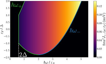
Figure 5. Joint density of states  for a gapped 2D anisotropic Rashba model with
  , and the absorption edges
  . The parameters used are
  ,
,  Å, and
  ,
,  for the effective masses.
Download figure:
Standard image High-resolution image4.2. First order spin current conductivity
According to the formula (3), the induced spin current response function of the anisotropic Rashba model becomes
where
Remarkably, the linear spin currents generated in this system will have electrons with out-of-plane spin orientations only. This a consequence of the breaking of TRS by the term  , which is a non null constant in the present model. This makes the product of matrix elements
  an odd (even) function in k-space when
  (
( ). Thus, the Kubo expression (3) integrates to a non zero value when
  only. The longitudinal components of the spin current conductivity (figure 6(a)) are proportional to the gap parameter,
  , and therefore they vanish for the gapless case. Moreover, these diagonal components are inversely proportional to
  , such that
  , as a consequence of the mass anisotropy. On the other hand, the Hall components are nonzero, regardless of the value of Δ, indicating the generation of a spin Hall effect in the gapped or ungapped system. In addition,
  , as can be seen in figure 6(b). The effect of the position of the Fermi level with respect to the gap, manifests through the critical energies
  . The variation of Fermi energy leads mainly to a change of the window
  , just like in JDOS.
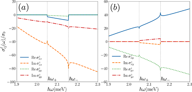
Figure 6. Longitudinal (a) and Hall (b) components of the linear spin current conductivity tensor  for a gapped anisotropic Rashba model, normalized to
  . The parameters used are
  ,
,  ,
,  ,
,  Å,
Å,  .
.
Download figure:
Standard image High-resolution imageIf  is the amplitude of the external field, the spin current can be written as the sum of a component along
  and a component perpendicular to it,
which reduces to  when
when  . Expression (28) suggests how the induced spin current could be manipulated through the frequency dependence of the tensor
  and the direction of the applied in-plane electric field.
4.3. SH spin current conductivity
For the SH spin current conductivity we obtain the following expressions from (6) (no sum over repeated indices is implied),
where  , A(x) is given by (27), and
A number of conclusions can be derived from these expressions. In contrast to the linear response, the above expressions imply that there is no z-polarized SH spin current induced in the system,  . On the other hand, equation (30) shows that if
  the longitudinal response
  describes a spin current with the spin oriented perpendicularly to the electric field (and to the spin current), while one with parallel spin orientation and current is possible when
  . The Hall components
  (29) generate spin currents with spin always oriented in the direction of the field (normal to the spin current), regardless of the presence of an energy gap. As for the components in (31),
  and
and  , they are associated to a nonlinear current with spin orientation parallel to it when
  , otherwise such an orientation is not fixed for
  .
.
The terms in braces in (29)–(31) involve the masses through the combination  only. Thus, the in-plane anisotropy becomes apparent in every non-zero tensor component through a factor of the type
  , with
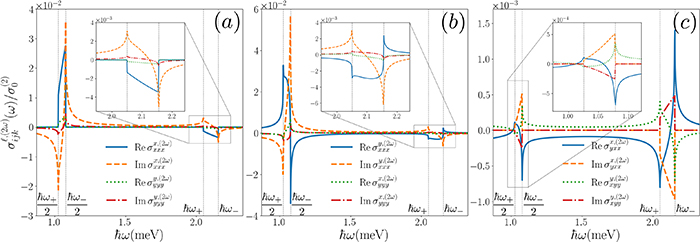
  or 3. Figure 7 shows the frequency dependence of the in-plane polarized SH components
  and
and  . As expected, the spectral structure around
  is now accompanied by new features around the subharmonics
  . The overall structure can be modified through Fermi energy variation, given the behavior of the functions
  observed in figure 5.
Figure 7. Second-harmonic spin current conductivity tensor  for a gapped 2D anisotropic Rashba model, which determines a spin current flowing in direction i, with the spin polarized along the direction
  , induced by the external field components j and l. In this system
  . (a) Longitudinal components with
  . (b) Longitudinal components with
  . (c) Hall components with
  . The parameters used are the same as in figure 6, and
  .
.
Download figure:
Standard image High-resolution image
The SH spin current response (29)–(31) presents characteristic differences with respect to the linear response, as is the case in the model of section 3. Diagonal components are present even in absence of an energy gap, subharmonic structure appears in the spectrum, and the spin polarization is no longer out-of-plane, so that a nonlinear spin Hall effect with in-plane spin orientation is generated. These features may be useful in nonlinear optical spintronic devices.
5. Summary
We calculated the spin conductivity tensors which characterize the electric-dipole induced spin currents at the fundamental and SH frequencies, in two anisotropic systems with SO interaction.
In the case of a 2DEG with R+D![$[hkl]$](https://content.cld.iop.org/journals/0953-8984/35/50/505301/revision3/cmacf74dieqn331.gif) , a time-reversal preserving system, the anisotropy arises from the interplay between the Rashba and Dresselhaus couplings, which in turn depends sensitively on the sample growth direction. For a given crystallographic orientation, the spin splitting of the states acquire a particular dependence on the direction in k-space. We show how this modify the spectrum of allowed optical transitions to explain the origin of the characteristic spectra displayed by the JDOS and the spin current responses at at ω and 2ω. As is known, the modulability of the Rashba strength, frequency tuning and the direction of the applied electric field, are mechanisms to manipulate the magnitude and direction of the induced linear and nonlinear spin current. Based on the crystal orientation dependence, our results suggest a new possibility, that is the selection of a particular response spectrum after a comparison between calculations for several growth directions. We found that the response functions
, a time-reversal preserving system, the anisotropy arises from the interplay between the Rashba and Dresselhaus couplings, which in turn depends sensitively on the sample growth direction. For a given crystallographic orientation, the spin splitting of the states acquire a particular dependence on the direction in k-space. We show how this modify the spectrum of allowed optical transitions to explain the origin of the characteristic spectra displayed by the JDOS and the spin current responses at at ω and 2ω. As is known, the modulability of the Rashba strength, frequency tuning and the direction of the applied electric field, are mechanisms to manipulate the magnitude and direction of the induced linear and nonlinear spin current. Based on the crystal orientation dependence, our results suggest a new possibility, that is the selection of a particular response spectrum after a comparison between calculations for several growth directions. We found that the response functions  and
and  vanish identically under the SU(2) symmetry conditions found in [45]. There are, however, additional conditions under which specific tensors components vanish, without the requirement of having a collinear SO vector field. Thus, by a proper choice of the growth direction and SO material parameters, one could select the polarization of the linear and SH spin currents according to the direction of flowing.
In the case of the anisotropic Rashba model studied in section 4, the anisotropy is that of a 2D free electron gas with different masses [59],  , in the presence of a Rashba type interaction which introduces different spin splitting along perpendicular directions [50]. To be comprehensive, the model includes an energy gap parameter, which breaks the TRS; when the gap is closed, the model reduces to that used in [51] to study the linear charge current response. The band structure offers distinct positions for the Fermi level (above, within, and below the gap), which define several distinguishable scenarios for the allowed optical interband transitions, characterized by the Fermi contours in each case. These manifest in contrasting ways in the linear and SH spin current response. The linear spin conductivity
  shows that only out-of-plane spin polarized currents develops (
 ), while the SH spin conductivity tensor
  gives rise to currents with spin orientation lying parallel to the plane of the electron gas (
 ). The longitudinal components
  are inversely proportional to
  , connected through the masses in the form
  , and vanishing for the gapless case. In contrast, the Hall components are non null regardless of the presence of a gap, depend on the masses through the geometric mean
  only, and satisfy
  . On the other hand, the SH components are proportional to the ratio of masses in the combination
  or
or  .
.
In summary, we investigated the spectral properties of the linear and nonlinear optical spin conductivities of two anisotropic models for SO coupled systems, and its dependence on a number of physical quantities like the exciting frequency, the position of the Fermi level, energy gap, mass anisotropy, SO strengths, Rashba and Dresselhaus couplings interplay for arbitrary sample growth directions, or the direction of the externally applied electric field, according to each case. The presence of anisotropy introduces optical signatures which in turn may be useful to identify or estimate some of these material parameters. In particular, the models illustrate the existence of the nonlinear spin Hall effect in systems with SO interaction, under the presence or absence of time-reversal symmetry. The results suggest different ways to manipulate the optically induced linear and SH spin current responses, which could find spintronic applications. We hope that this work will stimulate further investigations under more general conditions, such as the presence of extrinsic SO mechanisms or the use of a conserved spin current definition [54, 66].
Acknowledgment
D M-S acknowledges financial support from CONACYT (México).
Data availability statement
All data that support the findings of this study are included within the article (and any supplementary files).