Correlation effects on topological end-states in finite-size graphene nanoribbons in the GW approximation

Since its experimental isolation [1], graphene has been extensively studied owing in part to its unique electronic properties [2]. Macroscopically large graphene sheets are semi-metallic, i.e. with a zero electronic band gap. However, fragments of graphene of different sizes and shapes can display significantly different electronic properties compared to graphene, for example with the appearance of an electronic band gap. The spatial confinement in graphene fragments can also induce the emergence of magnetic properties [3]. In particular, graphene nanoribbons (GNRs) are of special interest since they can be synthesized with atomic precision [4–11]. The development of synthesis processes and theoretical studies [12–15] have opened new research directions where the electronic properties of GNRs can be tuned and engineered by structuring the GNRs. For instance, heterojunctions of different types of GNRs or chevron-types GNRs have prompted much interest in this field [16–20]. Interestingly, there is not full consensus in the literature regarding the electronic or magnetic properties of simple GNRs, due in large part to the difficulty of describing many-body effects in a sufficiently accurate manner. This paper addresses this issue by considering a GW treatment of the Hubbard model. This method has already been used to describe 2D carbon structures such as GNRs heterojunctions or small polycyclic aromatic hydrocarbons [16, 21] and it will be applied to finite-size GNRs in this work.

Armchair GNRs (AGNRs) are often categorized into three families, based on their specific electronic band-gap versus width dependence [12–14, 22] and defined by $N_\mathrm a = 3p$, $3p+1$, or $3p+2$ where $N_\mathrm a$ is the number of atoms across the width of the unit cells (UCs) and p is an integer. However, tight-binding (TB) and $\mathbf {k} \cdot \mathbf{p}$ approximations predict a zero band-gap (i.e. metallic AGNRs) for the $3p+2$ family [12, 13] and the TB approximation leads to the following hierarchy of the gaps: $\Delta_{3p} \geqslant \Delta_{3p+1} \gt \Delta_{3p+2} = 0$ [12]. In density functional theory (DFT), when considering local density approximation (LDA) or the GW correction over LDA, the smallest gaps are also the ones of the $3p+2$ family but they are predicted to be greater than zero (i.e. the AGNRs are non-metallic). What is more, the hierarchy of the two other families is inverted: $\Delta_{3p+1} \gt \Delta_{3p}$. It is important to note that the LDA + GW method we just invoked implies a GW treatment of the (long-range) Coulombic interaction between electrons. In our study, the GW approximation accounts for the many-body spin up–spin down interactions on the same atomic sites.

There are a several publications addressing the effect of adding a spin–spin interaction term to the TB Hamiltonian [14, 23, 24]. These studies investigated different parameterizations of an extended TB model (including the Hubbard term) for infinite AGNRs [23], the influence of U on the band gap of a finite seven-AGNR [24], and the competition between end states (ESs) and bulk states (BSs) in different small AGNRs [14]. Both [14, 23] employed a mean-field (MF) approximation whereas [24] implemented more advanced self-energy approximations.

The ES's of finite-size AGNRs are usually understood as topological states, originating from the change in Zak phase Z₂ at the interface of the AGNRs and the vacuum [10, 25, 26]. It has been shown in [16] that topological states due to such change in Zak phase in GNRs heterostructures are strongly affected by correlation effects. These correlations are thus expected to be of importance in the description of ES in finite-size AGNRs. However, a new topological classification using chiral symmetry was recently proposed and used for GNRs [26, 27]. This classification is based on the Z invariant and predicts the number of topological ES pairs to be Z for semiconducting AGNRs and Z − 1 for metallic AGNRs.

To the best of our knowledge, [14] is one of the few studies that investigated finite-size AGNRs using a MF Hubbard Hamiltonian for different widths and lengths. In this work, we extend the discussion the authors of the study initiated, including correlation via the GW approximation as well as comparing the effect of different U values. It appears important to us to study finite-size systems since they ultimately correspond to structures that are experimentally accessible [5, 10, 11]. This allows us to compare our theoretical computations to available published experiments. When considering total electronic contributions to the formation of scanning tunneling microscopy (STM) simulations, the GW corrections do not give a clear improvement, in terms of local density of states. However, we show that the spins contributions might be greatly affected when considering the different methods and the present study therefore suggests the experimental verification of the properties of AGNRs via spin-polarized STM in order to access quantities that appear to be most affected by correlation. In contrast, scanning tunneling spectroscopy (STS) experiments yield information that can be readily compared with total density of states and energy positions of the states. We were thus able to compare these quantities for MF and GW with experimental results. The GW corrections allow a much better description of the experimental results.

The rest of the article is organized as follows. In section 2 we introduce the model Hamiltonians as well as the Green's function method used. In section 3, we extend the study of [14] on the ES and BS of small AGNRs. We therefore contrast the effect of GW correlation and of MF approximation considered in [14] as well as the effect of increasing the interaction parameter U of the Hubbard model. In section 4, we compare our results to experiments and DFT computations in terms of local density of states and STM/STS simulations and experiments. We highlight the energy renormalisation of the ES in the GW approximation as well as the stronger localization of the ES.

2.1. Hubbard model

The Hubbard model is a popular model used to describe spin interaction effects in materials and in particular in graphene and graphene nanofragments [2, 3, 28]. The single-orbital Hubbard Hamiltonian is given by:

$$\begin{align} \hat{H}_\mathrm {Hubbard} = \left( -t \sum_{\lt ij\gt, \sigma} \hat{c}^\dagger_{i,\sigma} \hat{c}_{j,\sigma} + hc. \right) + U \sum_{i} \hat{n}_{i \uparrow} \hat{n} _{i\downarrow}, \end{align} \tag{ 1 }$$

where indices i and j label atomic sites, and the σ index refers to the spin the electron. $\hat{c}^\dagger_{i,\sigma}$ and $\hat{c}_{i,\sigma}$ are the creation and annihilation operators of an electron on site i with spin σ, and $\hat{n}_{i \sigma} = \hat{c}^\dagger_{i \sigma} \hat{c}_{i \sigma}$ is the density operator of electron on site i with spin σ. '$hc.$' stands for 'Hermitian conjugate' and $\lt\ldots\gt$ indicates that the sum only involves pairs of nearest-neighbor sites. t and U in equation (1) are the only two parameters of the single-orbital Hubbard model. The first one is the hopping parameter while the second one is the interaction parameter. If U = 0, the Hamiltonian is reduced to the single-orbital TB Hamiltonian [2, 3].

2.2. MF approximation

Treating exactly the Hubbard Hamiltonian for systems of hundreds of electrons is not tractable, due to the fast growing size of the many-body basis set [29–31]. To circumvent this limitation, a very common approximation of the Hubbard Hamiltonian is the MF approximation where the electron with a given spin on one site interacts with the mean density of the electrons of the opposite spin:

$$\begin{align} \begin{aligned} \hat{H}_\mathrm {Hub, MF} & = \left( -t \sum_{\lt ij\gt, \sigma} \hat{c}^\dagger_{i,\sigma} \hat{c}_{j,\sigma} + hc. \right) \\ & \quad +\sum_{i} U (\hat{n}_{i\uparrow} \langle \hat{n}_{i\downarrow} \rangle + \langle \hat{n}_{i\uparrow} \rangle \hat{n}_{i\downarrow} ), \end{aligned} \end{align} \tag{ 2 }$$

where $\langle \hat{n}_{i\sigma} \rangle$ is the mean value of the operator $\hat{n}_{i\sigma }$.

The eigen-states of the Hamiltonian in equation (2) are found self-consistently, starting from an initial guess for the mean values $\langle \hat{n}_{i\sigma} \rangle$. This approximation has the advantage that it can be expressed in the one-electron basis. It leads to a drastic reduction of the numerical resources needed but presents the caveat of neglecting all the correlation.

2.3. GW approximation

In order to describe correlated systems beyond the MF but at a smaller computational cost than that of the exact diagonalization, a number of approximations from the non-equilibrium Green's function framework have been developed such as T-matrix approximation, second-order Born approximation, GW approximation, etc [32–36]. In this study, we adopt the GW approximation, whose foundation is Dyson's equation:

$$\begin{align} G^{R} (\omega) = G^{R}_0 (\omega) + G^{R}_0 (\omega) \Sigma^{R} (\omega) G^{R} (\omega), \end{align} \tag{ 3 }$$

where G^R ₀ is the non-interacting retarded Green's function (computed using the MF solution), G^R is the exact retarded Green's function, and $\Sigma^{R}$ the retarded self-energy.

In the single-orbital basis, Dyson's equation is written in matrix form such that all quantities are matrices and products are matrix products. It is a frequency (i.e. energy) dependent equation. Note that we work in natural units, such that $\hbar = 1$ and ω is in energy units. The core of the GW description consists in approximating the self-energy as the product of G (Green's function) and W (screened potential). Dyson's equation is then solved self-consistently by computing an updated Green's function at each iteration, starting from the MF one. More details on the method and its implementation can be found in [16, 21, 29].

2.4. Observables from Green's functions

One can obtain spectral properties from either Green's function (G₀ or G). This includes local and total density of states (LDOS or $n_{i\sigma}(\omega)$ and DOS or $D(\omega)$). These quantities are expressed in terms of the Green's function as:

$$\begin{align} n_{i\sigma}(\omega) = \frac{1}{2\pi} A_{i\sigma,i\sigma} (\omega) \end{align} \tag{ 4 }$$

and

$$\begin{align} D(\omega) = \sum_{i\sigma} n_{i\sigma}(\omega), \end{align} \tag{ 5 }$$

where $A_{i\sigma,j\sigma^{^{\prime}}} (\omega) = -2\, {\text{Im}}(G^R_{i\sigma,j\sigma^{^{\prime}}}(\omega))$ is the spectral function.

The LDOS can be accessed experimentally as spatially-resolved $\mathrm dI/\mathrm dV$ images using STS. Working in interval of energies $[E_1,E_2]$, the calculation of $\mathrm dI/\mathrm dV$ involves non-diagonal terms of the Green's function. Using Tersoff–Hamann theory for an s-type tip [37, 38], the simulated $\mathrm dI/\mathrm dV$ maps are found according to the formula [16]:

$$\begin{align} \begin{aligned} \frac{\mathrm{d}{I}}{\mathrm{d}{V}} (x,y,z_0)& = \int_{E_1}^{E_2} \mathrm{d}{\omega} \sum_{ij} \sum_{\sigma \sigma^{\prime}} A_{i\sigma, j\sigma^{\prime}}(\omega) z_0^2 \\ & \quad \cdot \mathrm e^{\lambda^{-1} \vert\vec{r}-\vec{r_i}\vert} \mathrm e^{\lambda^{-1} \vert\vec{r}-\vec{r_j}\vert}, \end{aligned} \end{align} \tag{ 6 }$$

where z₀ is the tip's height of the simulated STS; λ is a length parameter that accounts for the spatial extension of localized orbitals; and $(x,y,z_0) = \vec{r}$ is the location where the STS is simulated and $\vec{r}_i$ are the atomic positions. We used the values $z_0 = 4$ Å and λ = 0.86 Å throughout this paper. The influence of these parameters on the simulated STS is a bit discussed in the SI.

We now isolate the contribution of only spin σ electrons to the simulated $\mathrm dI/\mathrm dV$ maps:

$$\begin{align} \begin{aligned} \frac{\mathrm{d}{I}}{\mathrm{d}{V}} \bigg|_\sigma (x,y,z_0)& = \int_{E_1}^{E_2} \mathrm{d}{\omega} \sum_{ij} A_{i\sigma, j\sigma} (\omega) z_0^2 \\ & \quad \cdot \mathrm e^{\lambda^{-1} \vert\vec{r}-\vec{r_i}\vert} \mathrm e^{\lambda^{-1} \vert\vec{r}-\vec{r_j}\vert}. \end{aligned} \end{align} \tag{ 7 }$$

These spin contributions to the total $\mathrm dI/\mathrm dV$ maps can be accessed experimentally using spin-polarized STM, potentially using a combination of several spectra [39–42].

This section is devoted to the theoretical investigation of the effect of using the GW approximation and of changing the Hubbard interaction parameter U on the properties of one representative AGNR system of each family. To facilitate a comparison with a previous study, we focus on seven-AGNR, nine-AGNR, and 11-AGNR since they have been studied in the TB and MF approximations of the Hubbard model in [14]. The authors of this research listed a number of observations that we will further discuss here. For instance, it was observed that:

• In contract to the ES, the BS energies are almost unaffected by the interaction term of the Hubbard model (U) when compared to the TB energies.
• The highest occupied molecular orbitals (HOMOs) and lowest unoccupied molecular orbitals (LUMOs) are ES for AGNRs with $\textrm{mod}(n,3) = 1$ and $\textrm{mod}(n,3) = 0$, while they can be BS for AGNRs with $\textrm{mod}(n,3) = 2$. In particular, the HOMOs and LUMOs are ES for seven-AGNRs and nine-AGNRs, with the difference between BS and ES in nine-AGNRs being smaller than in seven-AGNRs. In contrast, the HOMOs and LUMOs can be ES or BS (if the ribbon is long enough) for 11-AGNRs.

The number of ES can be predicted in the TB approximation in terms of the chiral topological invariant Z [26]. Both seven- and nine-AGNRs have Z = 1 and, since they are semiconducting, they are predicted to host Z = 1 pair of topological ES. We note that 11-AGNRs have Z = 2 but because they are metallic, they are predicted to have $Z-1 = 1$ pair of topological ES. All studied AGNRs in this section are thus predicted to have one pair of topological ES at the TB level.

3.1. Effects of GW correction with $U = 4/3\,t$

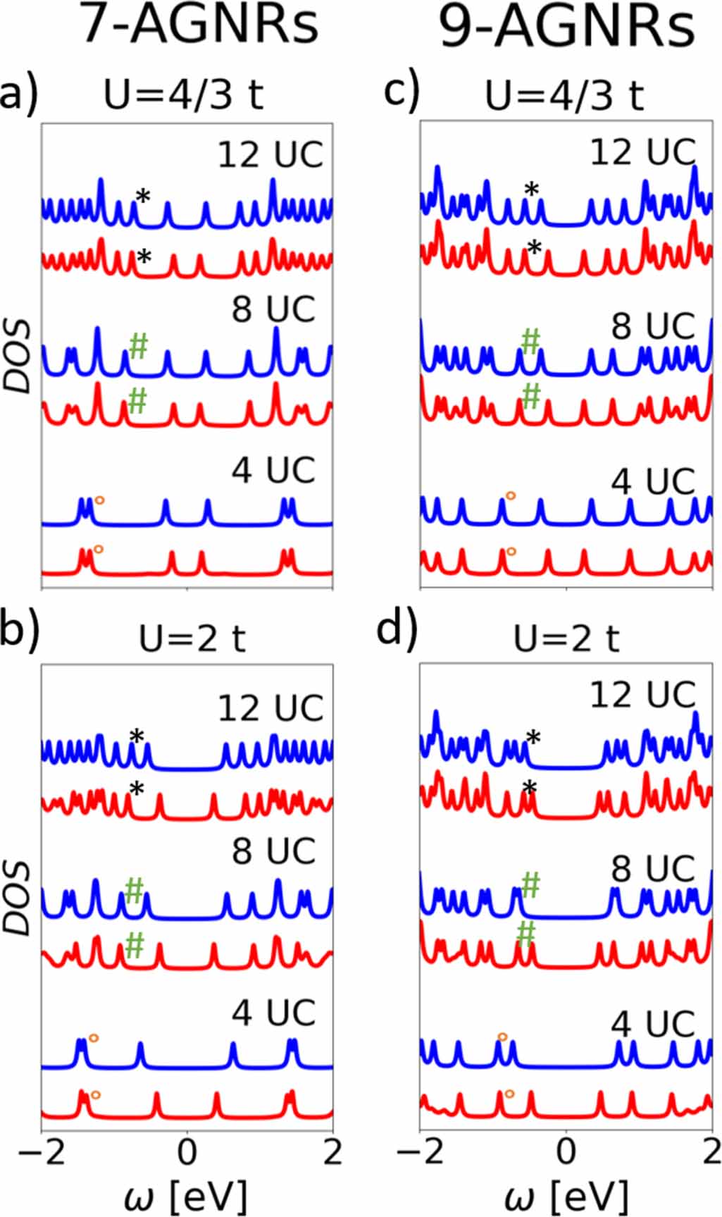
First, we start by considering the systems studied in [14] with the same model parameters, i.e. t = 2.7 eV and $U = 3.6\,\mathrm{eV} = 4/3\,t$, in order to assess the influence of the GW correction. Figure 1 shows the DOS obtained in the MF and GW approximations for seven-AGNRs (figure 1(a)), nine-AGNRs (figure 1(b)), and 11-AGNRs (figure 1(c)) for three different lengths: 4, 8, and 12 UCs.

Zoom In Zoom Out Reset image size

The HOMO and LUMO states of seven-AGNRs and nine-AGNRs are ES in both the MF approximation and GW correction (see figure 1, where the green dotted lines mark the BS and the other frontier states corresponding to ES). The effect of GW compared to MF for all AGNRs considered is mainly to shift the ES toward E_F , leaving the energies of BS almost unchanged. For the 11-AGNRs however, it was already observed in [14] that the HOMO and LUMO could be BS and not ES: this is the case for the 8 and 12 UC 11-AGNRs in the MF approximation (see figure 1 and [14]). A crossing between ES and BS thus occurs between the 4 UC and the 8 UC systems. In GW, since the BS energies are almost unchanged and the ES are shifted toward E_F , the crossing occurs for larger system length: while the crossing already occurred for the 8 UC in MF, the GW energies of ES and BS are very close to each other for this same length.

3.2. Effect of increasing the U parameter

In previous GW studies on carbon nanostructures [16, 21], the interaction parameter U had to be taken larger than the value used in [14] and in section 3.1 to match available experimental data. This is also the case here, as we will show below (see section 4). We thus now turn our interest to the effect of increasing this parameter from $U = 4/3\,t$ to $U = 2\,t$.

Figures 2 (a) and (b) show the DOS for the three selected lengths of seven-AGNRs in the MF and GW approximations. We observe that the BS energies are very similar for the two values (see peaks indicated in the figure). As for $U = 4/3\,t$, the ES's are more affected and shifted away from E_F when increasing the U parameter. This shift is higher in MF than in GW. In the particular case of seven-AGNRs, all HOMOs and LUMOs remain ES as in the case of $U = 4/3\,t$.

Zoom In Zoom Out Reset image size

Turning to nine-AGNRs, the same global trends are observed as for seven-AGNRs (see figures 2(c) and (d)). However, since the initial energy spacing between ES and BS is smaller for 9-AGNRs, a crossing between ES and BS is observed in the MF approximation from the 4 UC system to the 8 UC system. It appears that HOMOs and LUMOs are now BS for the 8 UC and 12 UC nine-AGNRs in the MF. The GW approximation however, still predicts the HOMOs and LUMOs to be ES for these systems. We thus show that inversions between BS and ES may occur in nine-AGNRs in addition to the observed inversion in [14] for 11-AGNRs.

The case of 11-AGNRs shows several similarities with the two first systems (see figure 1 in the SI for the densities of states). The main effect of increasing U is to shift the ES away from E_F . In the 11-AGNRs, the shift for the BS in MF is larger than for other systems but is still small compared to the shift of ES, being always more than three times smaller. This shift for BS is reduced when considering the GW approximation. The consequence of these observations is that the crossing between BS and ES occurs for smaller systems when increasing U, as for the nine-AGNRs. In MF, none of the three considered lengths exhibits ES as HOMO and LUMO, whereas it is only the case for the 4 UC system in GW (HOMOs and LUMOs being BS for 8 UC and 12 UC in GW).

We now focus on the seven-AGNRs that have been recently synthesized, characterized by STM/STS and studied theoretically by the means of ab initio simulations [11]. More specifically, the energy splitting of ESs $\Delta_{ZZ}$ in these nanoribbons was shown to be of significant magnitude compared with the BSs gap $\Delta_{AC}$. More precisely, the values $\Delta_{ZZ} \simeq$ 1.9–2 eV and $\Delta_{AC} \simeq$ 3–3.5 eV were found for the different investigated sizes of seven-AGNR (see figure 3 of [11]). This reference proposed an experimental strategy to transfer the nanoribbons from a Au(111) on which they were synthesized onto a NaCl monolayer, which is itself deposited on a a Au(111) substrate. This experimental proposal to make GNRs neutral and electronically decoupled from Au(111) is expected to approach free-standing properties of GNRs [43], this is why we considered this experimental study in particular.

The LDOS for the nearest peak below the Fermi level—which has been identified as being HOMO—and the peak of energy right under the HOMO (HOMO-1) are given at figure 3 for the MF and GW approximations with U parameters of $1.3\,t$, $2.5\,t$, and $3\,t$. For U parameters of the order of magnitude of t ($U = 1.3\,t$ on figure 3), the LDOS are hardly changed from MF to GW. Both MF and GW are in great agreement with DFT results from [11] and the HOMO is predicted to be an edge states while the HOMO-1 is predicted to be a BS (spread over the ribbon). When increasing U in MF, the HOMO tends to be less end-localized and, for $U = 3\,t$, the atoms at the middle of the two ends of the ribbons are not the most occupied atomic sites by the HOMO anymore. On the contrary, the HOMO-1 in MF tends to be more localized at the edges for larger values of U. This state also becomes less spatially symmetric for each spin channel. One observed that the effect of GW corrections is to further keep the edge-localized character of the HOMO state while U is increasing. This characteristic has the consequence that a larger range of U values could be considered when describing seven-AGNRs with the constraint of the HOMO and LUMO states to be edge-localized, as observed experimentally [11]. The extension of the possible U values to match with experiment or other methods was previously highlighted by us in [29] where we showed that the outset of an artificial phase transition induced by MF was shifted towards higher U values in GW, in a better agreement with exact results. We notice that for high U values, none of the approximations really reproduces the DFT results of [11]. However, DFT is also known for not taking into account correlation effects correctly.

Zoom In Zoom Out Reset image size

The simulated STM images of a longer seven-AGNR (10 UCs) are shown in figure 4 for U values of $1.3\,t$ and $2.5\,t$. Since STM simulations take into account both spin channels, we see that despite the fact that the spatial asymmetry of the LDOS increases for each spin, the total simulated STM maps remain essentially identical in GW between $U = 1.3\,t$ and $U = 2.5\,t$, while they are strongly modified in MF. Only the STM simulations corresponding to the edge-located HOMO are in agreement with the experimental data reported in [11], that is the one for small U ($1.3\,t$) in MF and both simulated STM maps for GW. Since the spatial asymmetry increases in spin channel for the LDOS (see figure 3), we believe that spin-polarized STM experiments could help determine the amount of correlation and compare different level of theory (model Hamiltonians and ab initio).

Zoom In Zoom Out Reset image size

The experimental spatial STM maps can be well reproduced by both MF and GW (figure 4) and one cannot determine which is a better approximation from these simulations. However, when looking at STM simulations of separate spin channels, a clearer difference can be observed for results obtained with small U values ($U = 1.3\,t$ on figure 5) and larger U values in the GW approximation ($U = 2.5\,t$ on figure 5). This should be understood as a fingerprint of the LDOS studied before and showed in figure 3. We therefore suggest that further experimental exploration of GNRs including spin-polarized STM experiments could be used, with the support of theoretical simulations, to look for the expression of many-body correlation effects. Moreover, it appears that a change in the parameters of the simulations such as the local orbital extension (or the height of the tip) could reveal more accurately the LDOS features (see figures 2 and 3 in the SI). These parameters can be used to describe different experimental set-ups such that there should exist experimental STM measurement parameters approaching LDOS features.

Zoom In Zoom Out Reset image size

We now focus on the simulation of STS measurements to describe the edge-states gap ($\Delta_{ZZ}$) as well as the BSs gap ($\Delta_{AC}$). In the Hubbard model, for a given $U/t$ ratio, the energy range of all the spectra can be scaled via the t parameter. Instead of focusing on absolute values of the two gaps ($\Delta_{ZZ}$ and $\Delta_{AC}$), we consider the ratio $R = \Delta_{ZZ}/\Delta_{AC}$, comparing it to experimental values of [11] (see figure 3(g) therein), reproduced as horizontal lines on figure 6(a). The evolution of R for the MF and GW approximations as a function of U, compared with the experimental ones for seven-AGNRs with $6, 8$ and 10 UCs is shown in figure 6(a). We see in this figure that for both approximations and for all lengths, R increases with U. The best U values are $U = 2\,t$ and $U = 2.3\,t$ for MF and GW approximations respectively.

Zoom In Zoom Out Reset image size

For an easier global comparison, the sums (over the three different lengths) of the absolute values of the errors of the R ratio of both approximations are compared with experiment in figure 6(b). This confirms that the best U values are $U = 2\,t$ for MF and $U = 2.3\,t$ for GW. Even if the agreement is slightly better at the GW minimum than at the MF minimum, the improvement does not appear to be significant, even if one can already see in figure 6(a) that the experimental ratios are reproduced better by GW with $U = 2.3\,t$ than by MF with $U = 2\,t$. An additional benefit of this comparison is to fix the U values at $U = 2\,t$ for MF and $U = 2.3\,t$ for GW for the following of this comparison with the experiment.

Having fixed these parameter ratios, we extended our comparison between MF and GW on one hand and experiment on the other, to include more peaks beyond the two gap values $\Delta_{ZZ}$ and $\Delta_{AC}$. Figure 7(a) shows the energy diagrams for the three different lengths of seven-AGNRs for the experiment, the MF and GW approximations for all peaks accessible from figure 3 of [11] (6, 8, and 9 peaks for the 6 UC, 8 UC and 10 UC systems respectively). Figure 7(b) shows the errors between MF or GW approximations and experiments. The errors have been summed up for 6, 8 and, 10 UCs seven-AGNRs in the limits of available experimental data (some lower and higher energy peaks are not visible for shorter seven-AGNRs in [11]). The hopping parameters t = 4.46 eV for MF and t = 4.22 eV have been found to minimize the total errors, so that we decided to show the results for these values. From the R ratios shown in figure 6, we concluded that the agreement for GW was slightly better than for MF. It is clear now that the inclusion of correlations in GW leads to better energy results than the MF approximation.

Zoom In Zoom Out Reset image size

We note that the hopping terms to reproduce the experimental results in both approximations are relatively large (between 4 eV and 4.5 eV) compared to values usually found in the literature to describe graphene (between 2.7 eV and 3.2 eV) [2, 3, 44]. This is related to the renormalization of the hopping integral in a Hubbard model. Indeed, the typical way to find a value for the hopping parameter is to compute electronic properties such as the dispersion relation and to compare and fit it to ab initio computations [2, 45]. In these works, the dispersion relation are compared between the TB approximation and ab initio computations, meaning that the interaction term of the Hubbard Hamiltonian is not included. The inclusion of U modifies the relation dispersion of graphene and can open a band gap [28].

The hopping term in the Hubbard Hamiltonian is responsible for electron delocalization. On the other hand, local electronic interaction introduced with the U parameter tends to induce a localization of the electrons [46]. Adding non-local interaction terms (limited to nearest-neighbor), one ends up with the extended Hubbard model (EHM) defined by:

$$\begin{align} H_\mathrm{EHM} = \left( -t \Sigma_{\langle i,j \rangle, \sigma} c^\dagger_{i\sigma} c_{j\sigma} + hc. \right) + U \Sigma_i n_{i\uparrow} n_{i\downarrow} + \frac{V}{2} \Sigma_{\langle i,j \rangle} n_i n_j, \end{align} \tag{ 8 }$$

with V being the non-local nearest-neighbor interaction parameter.

The non-local interaction term tends to delocalize the electrons as the hopping term and it has been shown that the EHM can be mapped toward an EHM, setting V = 0 and decreasing the ratio $U/t$ [46, 47]. This can be understood as switching off a term that tends to delocalize electrons (non-local interactions) but increasing the other term responsible for delocalization (the hopping term). The EHM was studied for graphene in [47] and the following parameters were found: t = 2.8 eV, $U = 3.63\,t$, and $V = 2.03\,t$. Using these values in the proposed mapping of [46], one ends up with an effective Hubbard model with parameters t = 3.16 eV to t = 5.80 eV and $U = 1.82\,t$ to $U = 3.33\,t$. These values are compatible with the ones we used in this paper.

To sum up: the seemingly large hopping parameter found to optimize the match with experiment can be explained by the fact that we neglected non-local interactions and used the Hubbard model (introducing local interactions) and, doing so, the hopping parameter has to be renormalized, according to [46, 47].

In summary, we applied the GW approximation developed in [16, 21] to study the effect of a many-body Hubbard-type treatment of finite-size AGNRs. We first extended the theoretical study of [14] that considered the description of the AGNRs using the Hubbard model in the MF approximation for an interaction parameter $U = 4/3\,t$. We showed that the GW approximation mainly affects the ES whereas the BS are less affected. We observed that GW tends to reduce the gap between ESs in the considered AGNRs, affecting the effect of 'competition' between ES and BS to be the HOMO and LUMO. In particular, the crossing between these states when increasing the length of an 11-AGNR turned out to be at smaller length in GW than in MF. We then explored the effect of increasing the U interaction term of the Hubbard model. The main effect was also observed on the ES, increasing the ES gap ($\Delta_{ZZ}$) and therefore changing the ratio between ES and BS gaps ($\Delta_{ZZ} /\Delta_{AC}$) as well as potentially affecting the HOMO and LUMO. More specifically, we showed that it is possible to have BS as HOMO and LUMO in nine-AGNRs, in the MF approximation. It is not the case for GW, that predicts a larger range of U resulting in ES as HOMO and LUMO.

We considered in more details the seven-AGNRs and compared our model predictions to experimental data of recently synthesized seven-AGNRs of [11]. This methodology yields very different results than other experimental studies that we were able to quantitatively reproduce theoretically within the GW approximation with very good agreement. The parameters found in our study are significantly larger than the ones usually employed in TB or Hubbard model for the description of graphene [2, 3, 16, 44]. Whereas DFT based methods are largely used to describe carbon nanosystems, they are known to not account accurately for correlation effects, specifically the spin–spin correlation considered here in the Hubbard model.

In this present work, we described AGNRs with a single-band Hubbard model, assuming edge passivation via hydrogen for all carbon atoms. However, AGNRs might be synthesized with other end terminations such as dangling bonds or di-hydrogenation [8, 48] but also with nitrogen substitution [49]. For example, it was observed that di-hydrogenation have an impact on the BS band gap [48]. Different ways of modeling such end modifications are been proposed including adapted modification of the on-site potential [48, 50–61]. The investigation of the impact of the nano-ribbon terminations on band gaps and on topological ES is a natural extension of the present work and is of great importance for further technological use.

A H is a Research Fellow of the Fonds de la Recherche Scientifique—FNRS. This research used resources of the 'Plateforme Technologique de Calcul Intensif (PTCI)' (www.ptci.unamur.be) located at the University of Namur, Belgium, and of the Université catholique de Louvain (CISM/UCL) which are supported by the F R S-FNRS under the convention No. 2.5020.11. The PTCI and CISM are member of the 'Consortium des Équipements de Calcul Intensif (CÉCI)' (www.ceci-hpc.be).

The data cannot be made publicly available upon publication because they are not available in a format that is sufficiently accessible or reusable by other researchers. The data that support the findings of this study are available upon reasonable request from the authors.