Implementation strategies in phonopy and phono3py

As shown in figure 1, a crystal model is defined by a collection of unit cells periodically repeated in the three directions of space. Each unit cell contains atoms. We normally choose a conventional set of basis vectors to span the unit cell, $(\mathbf{a}, \mathbf{b}, \mathbf{c})$, so that it naturally represents the crystal symmetry along with the choice of the origin of atomic positions [5]. Positions of atoms are represented either in Cartesian coordinates or in crystallographic coordinates. Denoting the crystallographic coordinates of an atom as $\boldsymbol{x} = (x_1,x_2,x_3)^\intercal$, its position R is given by

$$\begin{align} \mathbf{R} & = x_1 \mathbf{a} + x_2 \mathbf{b} + x_3 \mathbf{c} \nonumber \\ & = (\mathbf{a}, \mathbf{b}, \mathbf{c}) \begin{pmatrix} x_{1} \\ x_{2} \\ x_{3} \end{pmatrix} \nonumber \\ & = (\mathbf{a}, \mathbf{b}, \mathbf{c}) \boldsymbol{x}. \end{align} \tag{ 1 }$$

In the above equation, if the basis vectors are represented using column vectors containing their Cartesian components, then $(\mathbf{a}, \mathbf{b}, \mathbf{c})$ becomes a matrix, and R a column vector containing the Cartesian coordinates of the atomic position vector,

$$\begin{align} \begin{pmatrix} \mathbf{R}_x \\ \mathbf{R}_y \\ \mathbf{R}_z \end{pmatrix} = \begin{pmatrix} \mathbf{a}_x & \mathbf{b}_x & \mathbf{c}_x \\ \mathbf{a}_y & \mathbf{b}_y & \mathbf{c}_y \\ \mathbf{a}_z & \mathbf{b}_z & \mathbf{c}_z\end{pmatrix} \begin{pmatrix} x_{1} \\ x_{2} \\ x_{3} \end{pmatrix}. \end{align} \tag{ 2 }$$

In the following we will use both representations. Depending on the context, $(\mathbf{a}, \mathbf{b}, \mathbf{c})$ can therefore be considered as a row vector containing three elements of a vector space, or a 3 by 3 matrix.

Zoom In Zoom Out Reset image size

It is assumed that elements of x are in the interval $[0, 1)$ to describe the structure. However it is often the case that we have to compare two positions of atoms which may be in different unit cells, possibly after a space group operation. For example, to identify two coordinates x and $\boldsymbol{x}^{\prime}$ which correspond to the same location within the unit cell, but are possibly shifted by a lattice vector, it is convenient to bring each element of the difference $\Delta\boldsymbol{x} = \boldsymbol{x}^{\prime} -\boldsymbol{x}$ into the interval $[-0.5, 0.5)$ and then confirm that the length of $\Delta\boldsymbol{x}$ is smaller than a tolerance ε. This is implemented in the phonopy and phono3py codes everywhere by rounding components of $\Delta\boldsymbol{x}$ to the nearest integer ($\text{nint}(\Delta\boldsymbol{x})$) and checking $\left|(\mathbf{a}, \mathbf{b}, \mathbf{c}) [\Delta\boldsymbol{x} - \text{nint}(\Delta\boldsymbol{x})] \right| \lt \epsilon$.

Various symmetries of crystals and phonons are used in the phonopy and phono3py codes. The most important one is the space group symmetry. A space group operation is composed of a (proper or improper) rotation $\mathcal{S}$ and a translation τ. It is often written with a composite notation $(\mathcal{S},\tau)$ which sends position R to

$$\begin{align} \mathbf{R}^{\prime}=(\mathcal{S},\tau)\mathbf{R}\equiv\mathcal{S}\mathbf{R}+\tau. \end{align} \tag{ 3 }$$

Using crystallographic coordinates this is written as

$$\begin{align} (\mathbf{a}, \mathbf{b}, \mathbf{c}) \boldsymbol{x}^{\prime} = \mathcal{S} (\mathbf{a}, \mathbf{b}, \mathbf{c}) \boldsymbol{x}+ (\mathbf{a}, \mathbf{b}, \mathbf{c}) \boldsymbol{w} \end{align} \tag{ 4 }$$

or

$$\begin{align} \boldsymbol{x}^{\prime} & =(\mathbf{a}, \mathbf{b}, \mathbf{c})^{-1} \mathcal{S} (\mathbf{a}, \mathbf{b}, \mathbf{c}) \boldsymbol{x}+ \boldsymbol{w} \nonumber \\ & \equiv \boldsymbol{S} \boldsymbol{x} + \boldsymbol{w}, \end{align} \tag{ 5 }$$

where S can be shown to be a unimodular matrix. w contains the components of the translation vector in the crystallographic basis. If Cartesian coordinates were used instead, the matrix representing the rotation would be orthogonal. Representing the space group by $\mathbb{S} = \{(\mathcal{S},\tau)\}$, the crystallographic point group is given by $\mathbb{P} = \{\mathcal{S}|(\mathcal{S},\tau) \in \mathbb{S}\}$. An example of space group operation is shown in figure 2. The crystal structure overlaps with itself after a rotation of 60^∘ along the z axis and a $+\frac{1}{2}\mathbf{c}$ shift. Therefore

$$\begin{align} \boldsymbol{S}= \begin{pmatrix} 1 & \bar{1} & 0 \\ 1 & 0 & 0 \\ 0 & 0 & 1 \end{pmatrix}, \boldsymbol{w}= \begin{pmatrix} 0 \\ 0 \\ 1/2 \end{pmatrix}, \end{align} \tag{ 6 }$$

must be a space group operation. It means that any atom in the unit cell at point x is sent by the space group operation to a new point

$$\begin{align} \boldsymbol{x}^{\prime} = \begin{pmatrix} 1 & \bar{1} & 0 \\ 1 & 0 & 0 \\ 0 & 0 & 1 \end{pmatrix} \boldsymbol{x} + \begin{pmatrix} 0 \\ 0 \\ 1/2 \end{pmatrix}. \end{align} \tag{ 7 }$$

The new point $\boldsymbol{x}^{\prime}$ can be located out of the original unit cell, but an atom with the same atomic type must be found at this new location.

Zoom In Zoom Out Reset image size

In most cases, a unit cell as described in section 2.1 is used as the input crystal structure model of a phonon calculation. The most plausible choice of the unit cell is either a primitive cell or a conventional unit cell. The former represents the minimum unit of periodicity of a crystal lattice. It is therefore the one used for Fourier expansions and is necessary for a reciprocal space representation of phonon properties. The Bloch theorem evidenced this lattice translational symmetry. The latter follows the crystallographic convention. Although it provides intuitive shapes of the unit cells (cubic, hexagonal, etc), it may contain several lattice points. Figure 3 shows the conventional unit cell and a primitive cell for silicon crystallized within the face-centred-cubic structure.

Zoom In Zoom Out Reset image size

The conventional unit cell structure is uniquely defined to follow the crystallographic convention, [5] within the freedom due to Euclidean normalizer [5]. On the other hand, the choice of the primitive cell is not unique. This is inconvenient for a systematic handling of crystal structure models in phonon calculations. Therefore, phonopy suggests a predefined transformation matrix $\boldsymbol{P}_\text{prim}$ from the conventional unit cell to the primitive cell. $\boldsymbol{P}_\text{prim}$ is used as

$$\begin{align} (\mathbf{a}_\text{p}, \mathbf{b}_\text{p}, \mathbf{c}_\text{p}) = (\mathbf{a}_\text{c}, \mathbf{b}_\text{c}, \mathbf{c}_\text{c})\boldsymbol{P}_\text{prim}, \end{align} \tag{ 8 }$$

where $(\mathbf{a}_\text{p}, \mathbf{b}_\text{p}, \mathbf{c}_\text{p})$ are the basis vectors of the primitive cell and $(\mathbf{a}_\text{c}, \mathbf{b}_\text{c}, \mathbf{c}_\text{c})$ those of the conventional unit cell. The choices of the transformation matrices used in the phonopy and phono3py codes are shown in table 1. For example, the transformation matrix used for silicon in figure 3 is $\boldsymbol{P}_\text{prim} = \boldsymbol{P}_F$. These matrices are equivalent to those presented in table 2 of [6] although those are given for the reciprocal space basis vectors.

Table 1. Choices of transformation matrices $\boldsymbol{P}_\text{prim}$ of equation (8) used in the phonopy and phono3py codes. The subscripts X of the matrices P _X indicate the centring types: A, B, C for the base centring types, I and F for the body and face centring types, respectively, and R for the (obverse) rhombohedral centring type.

$\boldsymbol{P}_A = \begin{pmatrix} 1 & 0 & 0 \\ 0 & \frac{1}{2} & \bar{\frac{1}{2}} \\ 0 & \frac{1}{2} & {\frac{1}{2}} \\ \end{pmatrix}$,	$\boldsymbol{P}_B = \begin{pmatrix} \frac{1}{2} & 0 & \bar{\frac{1}{2}} \\ 0 & 1 & 0 \\ \frac{1}{2} & 0 & {\frac{1}{2}} \\ \end{pmatrix}$,	$\boldsymbol{P}_C = \begin{pmatrix} \frac{1}{2} & \frac{1}{2} & 0 \\ \bar{\frac{1}{2}} & \frac{1}{2} & 0 \\ 0 & 0 & 1 \\ \end{pmatrix}$,
$\boldsymbol{P}_I = \begin{pmatrix} \bar{\frac{1}{2}} & \frac{1}{2} & \frac{1}{2} \\ {\frac{1}{2}} & \bar{\frac{1}{2}} & \frac{1}{2} \\ {\frac{1}{2}} & \frac{1}{2} & \bar{\frac{1}{2}} \\ \end{pmatrix}$,	$\boldsymbol{P}_F = \begin{pmatrix} 0 & \frac{1}{2} & \frac{1}{2} \\ {\frac{1}{2}} & 0 & \frac{1}{2} \\ {\frac{1}{2}} & \frac{1}{2} & 0 \\ \end{pmatrix}$,	$\boldsymbol{P}_R = \begin{pmatrix} \frac{2}{3} & \bar{\frac{1}{3}} & \bar{\frac{1}{3}} \\ \frac{1}{3} & \frac{1}{3} & \bar{\frac{2}{3}} \\ \frac{1}{3} & \frac{1}{3} & \frac{1}{3} \\ \end{pmatrix}$.

The crystal lattice is defined as the set of integer linear combinations of primitive lattice vectors. A lattice vector R_l can therefore be written as

$$\begin{align} \mathbf{R}_l = l_1\mathbf{a}_\text{p} + l_2\mathbf{b}_\text{p} + l_3\mathbf{c}_\text{p}= (\mathbf{a}_\text{p}, \mathbf{b}_\text{p}, \mathbf{c}_\text{p}) \boldsymbol{l} \;\; (l_i \in \mathbb{Z}). \end{align} \tag{ 9 }$$

In figure 1, if the unit cell is assumed to be primitive, then figure 1(c) shows the crystal lattice. The lattice point may then be chosen to coincide with the origin of each unit cell. Sometimes it is also useful to regard the crystal lattice as generated using the lattice translations of the space group, $(\boldsymbol{I},\boldsymbol{t})$, where I and t denote the identity operation and lattice translation, respectively.

The crystal structure, and the symmetry explained above, are defined in direct (real) space. In this section, crystallography is briefly summarized in reciprocal space. This is quite useful for our purpose since phonons are described in reciprocal space using wave vectors. It is convenient to introduce a reciprocal lattice whose basis vectors $(\mathbf{a}_\text{p}^*, \mathbf{b}_\text{p}^*, \mathbf{c}_\text{p}^*)$ are solutions of the equation

$$\begin{align} (\mathbf{a}_\text{p}, \mathbf{b}_\text{p}, \mathbf{c}_\text{p})^{\intercal} (\mathbf{a}_\text{p}^*, \mathbf{b}_\text{p}^*, \mathbf{c}_\text{p}^*) = 2 \pi \boldsymbol{1}. \end{align} \tag{ 10 }$$

This equation can be solved to give

$$\begin{align} \mathbf{a}_\text{p}^* = 2\pi \frac{\mathbf{b}_\text{p} \times \mathbf{c}_\text{p}}{V_\text{c}}, \;\; \mathbf{b}_\text{p}^* = 2\pi \frac{\mathbf{c}_\text{p} \times \mathbf{a}_\text{p}}{V_\text{c}}, \;\; \mathbf{c}_\text{p}^* = 2\pi \frac{\mathbf{a}_\text{p} \times \mathbf{b}_\text{p}}{V_\text{c}}, \end{align} \tag{ 11 }$$

where $V_\text{c}\ =\ \mathbf{a}_\text{p} \cdot (\mathbf{b}_\text{p} \times \mathbf{c}_\text{p})\ =\ \mathbf{b}_\text{p} \cdot (\mathbf{c}_\text{p} \times \mathbf{a}_\text{p})\ =\ \mathbf{c}_\text{p} \cdot (\mathbf{a}_\text{p} \times \mathbf{b}_\text{p})$. The reciprocal lattice points are then obtained from the integer linear combinations of reciprocal basis vectors,

$$\begin{align} \mathbf{G} = G_1\mathbf{a}_\text{p}^* + G_2\mathbf{b}_\text{p}^* + G_3\mathbf{c}_\text{p}^*= (\mathbf{a}_\text{p}^*, \mathbf{b}_\text{p}^*, \mathbf{c}_\text{p}^*) \boldsymbol{G} \;\; (G_i \in \mathbb{Z}). \end{align} \tag{ 12 }$$

Similarly to the atomic positions R, wave vectors q are defined from real linear combinations of the reciprocal lattice vectors,

$$\begin{align} \mathbf{q} = q_1\mathbf{a}_\text{p}^* + q_2\mathbf{b}_\text{p}^* + q_3\mathbf{c}_\text{p}^* =(\mathbf{a}_\text{p}^*, \mathbf{b}_\text{p}^*, \mathbf{c}_\text{p}^*) \boldsymbol{q} . \end{align} \tag{ 13 }$$

If the q_i are restricted to the interval $[0,1)$, a primitive cell of reciprocal space is obtained.

If we consider a component of a Fourier expansion, $f_{\mathbf{q}}(\mathbf{R}) = \mathrm e^{i \mathbf{q}\cdot \mathbf{R}}$, it is transformed by an operation of the crystallographic point group to the function

$$\begin{align} \mathcal{S} f_{\mathbf{q}}(\mathbf{R}) & = f_{\mathbf{q}}(\mathcal{S}^{-1}\mathbf{R})= \mathrm e^{i \mathbf{q}\cdot \mathcal{S}^{-1} \mathbf{R}}= \mathrm e^{i \mathcal{S}\mathbf{q}\cdot \mathcal{S}\mathcal{S}^{-1} \mathbf{R}}= \mathrm e^{i \mathcal{S}\mathbf{q}\cdot \mathbf{R}} \nonumber \\ & = f_{\mathcal{S}\mathbf{q}}(\mathbf{R}). \end{align} \tag{ 14 }$$

For this reason, the image of a wave vector through an operation of the crystallographic point group is defined to be

$$\begin{align} \mathbf{q}^{\prime}=\mathcal{S}\mathbf{q} \Longleftrightarrow (\mathbf{a}_\text{p}^*, \mathbf{b}_\text{p}^*, \mathbf{c}_\text{p}^*) \boldsymbol{q}^{\prime} & = \mathcal{S} (\mathbf{a}_\text{p}^*, \mathbf{b}_\text{p}^*, \mathbf{c}_\text{p}^*) \boldsymbol{q} \end{align} \tag{ 15 }$$

or

$$\begin{align} \boldsymbol{q}^{\prime} & = (\mathbf{a}_\text{p}^*, \mathbf{b}_\text{p}^*, \mathbf{c}_\text{p}^*)^{-1} \mathcal{S} (\mathbf{a}_\text{p}^*, \mathbf{b}_\text{p}^*, \mathbf{c}_\text{p}^*) \boldsymbol{q} \end{align} \tag{ 16 }$$

$$\begin{align} & = (\mathbf{a}_\text{p}, \mathbf{b}_\text{p}, \mathbf{c}_\text{p})^{\intercal} \mathcal{S} (\mathbf{a}_\text{p}, \mathbf{b}_\text{p}, \mathbf{c}_\text{p})^{-\intercal} \boldsymbol{q} \end{align} \tag{ 17 }$$

$$\begin{align} & = \boldsymbol{S}^{-\intercal}\boldsymbol{q}. \end{align} \tag{ 18 }$$

The set $\{\boldsymbol{S}^{-\intercal} \boldsymbol{q}\}$ with S in the crystallographic point group $\{\boldsymbol{S}\}$ is called the star of q.

Atoms vibrate in the vicinity of their equilibrium positions in crystals. Instantaneous and equilibrium positions of atoms in crystals are denoted by $\mathbf{R}_{l\kappa}$ and $\mathbf{R}^0_{l\kappa}$, respectively, where l and κ are used to label the lattice points and atoms in the primitive cell of l, respectively. Displacements of atoms are written as $\mathbf{u}_{l\kappa} = \mathbf{R}_{l\kappa} - \mathbf{R}^0_{l\kappa}$.

In this review, we define the dynamical matrix as [7]

$$\begin{align} D_{{\kappa}\alpha,{\kappa}^{\prime} \alpha ^{\prime}}(\mathbf{q}) = \frac{1}{\sqrt{m_{\kappa}m_{{\kappa}^{\prime}}}} \sum_{l^{\prime}} \Phi_{0{\kappa}\alpha,l^{\prime}{\kappa}^{\prime} \alpha^{\prime}} \mathrm e^{i{\mathbf{q} \cdot (\mathbf{R}^0_{l^\prime{\kappa}^{\prime}} - \mathbf{R}^0_{0{\kappa}})}}. \end{align} \tag{ 19 }$$

α and m_κ denote the index of the Cartesian coordinates and the mass of the atom κ, respectively. $\Phi_{l{\kappa}\alpha,l^{\prime}{\kappa}^{\prime}\alpha^{\prime}}$ are the harmonic force constants, defined as the second derivative of the energy with respect to atomic positions, and evaluated at the equilibrium positions [7]. Phonon frequency $\omega_{\mathbf{q}\nu}$ and eigenvector $W_{\kappa\alpha}(\mathbf{q}\nu)$ are obtained as the solution of the eigenvalue equation of the dynamical matrix in equation (19), which is written as

$$\begin{align} \sum_{\kappa^{^{\prime}}\alpha^{^{\prime}}} D_{{\kappa}\alpha,{\kappa}^{^{\prime}}\alpha^{^{\prime}}}(\mathbf{q}) W_{\kappa^{\prime}\alpha^{\prime}}(\mathbf{q}\nu) = \omega^2_{\mathbf{q}\nu} W_{\kappa\alpha}(\mathbf{q}\nu). \end{align} \tag{ 20 }$$

ν labels the phonon band index, and the composite index $\mathbf{q}\nu$ is used to consider a phonon mode.

Equation (20) can also be written in matrix form as

$$\begin{align} \mathrm{D}(\mathbf{q}) \mathrm{W}(\mathbf{q}) = \mathrm{W}(\mathbf{q}) \Omega^2(\mathbf{q}), \end{align} \tag{ 21 }$$

or, because $\mathrm{D}(\mathbf{q})$ is hermitian,

$$\begin{align} \mathrm{D}(\mathbf{q}) = \mathrm{W}(\mathbf{q}) \Omega^2(\mathbf{q}) \mathrm{W}^\dagger(\mathbf{q}), \end{align} \tag{ 22 }$$

where $\Omega^2(\mathbf{q})$ is the diagonal matrix whose diagonal elements are $\omega^2_{\mathbf{q}\nu}$. Each column of $\mathrm{W}(\mathbf{q})$ contains an eigenvector $W_{\kappa\alpha}(\mathbf{q}\nu)$ corresponding to a different band index ν. Elements of each column are ordered as $(W_{\kappa_1 x}, W_{\kappa_1 y}, W_{\kappa_1 z}, \ldots, W_{\kappa_{n_\text{a}} x}, W_{\kappa_{n_\text{a}} y}, W_{\kappa_{n_\text{a}} z})$, where n_a is the number of atoms in the primitive cell.

Because $D_{{\kappa}\alpha,{\kappa}^{\prime}\alpha^{\prime}}(\mathbf{q}) = D^*_{{\kappa}\alpha,{\kappa}^{\prime}\alpha^{\prime}}(-\mathbf{q})$, we have

$$\begin{align} \omega_{\mathbf{q\nu}} = \omega_{\mathbf{-q\nu}}, \end{align} \tag{ 23 }$$

and we can choose

$$\begin{align} W_{\kappa\alpha}(\mathbf{q}\nu) = W^*_{\kappa\alpha}(-\mathbf{q}\nu). \end{align} \tag{ 24 }$$

Moreover eigenvalues and eigenvectors inherit symmetry properties of the force constants. It can be shown [8] that under a space group operation $(\mathcal{S},\tau)$ the eigenvalues and eigenvectors transform as

$$\begin{align} & \omega_{\mathcal{S} \mathbf{q\nu}} = \omega_{\mathbf{q\nu}}, \end{align} \tag{ 25 }$$

$$\begin{align} & \mathbf{W}_{\kappa^{\prime}}(\mathcal{S} \mathbf{q}\nu) = \mathcal{S} \mathbf{W}_{\kappa}(\mathbf{q}\nu) \mathrm e^{-i\mathcal{S} \mathbf{q}\cdot \tau}, \end{align} \tag{ 26 }$$

where $\mathbf{W}_{\kappa}(\mathbf{q}\nu)$ represents the phonon eigenvector of atom κ in Cartesian coordinates, and $\kappa^{\prime}$ is the image of atom κ under the space group operation.

An actual displacement can be described from a linear combination of phonon eigenvectors. This defines the phonon coordinates $Q(\mathbf{q}\nu)$ as

$$\begin{align} u_{l{\kappa}\alpha} & = \sum_{\mathbf{q}\nu} Q(\mathbf{q}\nu) \frac{1}{\sqrt{Nm_{\kappa}}} W_{\kappa\alpha}(\mathbf{q}\nu) \mathrm e^{i\mathbf{q} \cdot \mathbf{R}^0_{l{\kappa}}} \end{align} \tag{ 27 }$$

$$\begin{align} & = \sum_{\mathbf{q}\nu} Q(\mathbf{q}\nu) u_{l{\kappa}\alpha}(\mathbf{q}\nu), \end{align} \tag{ 28 }$$

where N is the number of lattice points in crystal. $u_{l{\kappa}\alpha}(\mathbf{q}\nu)$ is defined for the purpose of convenience in the following sections. The previous equation can be inverted to give

$$\begin{align} Q(\mathbf{q}\nu)= \sum_{l{\kappa}\alpha} u_{l{\kappa}\alpha} \sqrt{\frac{m_{\kappa}}{N}} W^{*}_{\kappa\alpha}(\mathbf{q}\nu) \mathrm e^{-i\mathbf{q} \cdot \mathbf{R}^0_{l{\kappa}}}. \end{align} \tag{ 29 }$$

Symmetry property of phonons in reciprocal space is best represented in the BZ [6, 8–12]. In the phonopy and phono3py codes, the BZ is defined as a Wigner–Seitz cell of the reciprocal lattice. To check if a q point belongs to the BZ we proceed as follows. First the basis vectors of the Niggli cell [13–16] are determined. The Niggli cell is a cell with the shortest possible reciprocal basis vectors. Then using integer linear combinations of those Niggli basis vectors, we search for the shortest $|\mathbf{q}+ \mathbf{G}|$. Finally $\mathbf{q} + \mathbf{G}$ is used as the q point in the BZ.

Three q points are needed for the three-phonon scattering considered in the phono3py code. In case one or more of those three points is on the BZ surface, we choose the translationally equivalent points on the BZ surface which minimize $|\mathbf{q} + \mathbf{q}^{\prime} + \mathbf{q}^{^{\prime\prime}}|$.

As an example, the BZ of β-Si₃N₄ is presented in figure 4. The basal plane has the hexagonal shape and $\mathbf{c}_\text{p}^*$ is longer than $\mathbf{a}_\text{p}^*$ and $\mathbf{b}_\text{p}^*$ because $\mathbf{c}_\text{p}$ is shorter than $\mathbf{a}_\text{p}$ and $\mathbf{b}_\text{p}$. By definition, $\mathbf{a}_\text{p}^*/2$, $\mathbf{b}_\text{p}^*/2$, and $\mathbf{c}_\text{p}^*/2$ are located on the BZ surface. The high symmetry points and paths in the BZ have special symbols as shown in figure 4(b) [6].

Zoom In Zoom Out Reset image size

In the phonopy and phono3py codes, the supercell approach is employed. The supercell is defined by multiple primitive cells, so that the basis vectors of the supercell $(\mathbf{a}_\text{s}, \mathbf{b}_\text{s}, \mathbf{c}_\text{s})$ can be represented as the image of the primitive cell basis vectors through an integer matrix $\boldsymbol{M}_{\text{p}\rightarrow\text{s}}$,

$$\begin{align} (\mathbf{a}_\text{s}, \mathbf{b}_\text{s}, \mathbf{c}_\text{s}) = (\mathbf{a}_\text{p}, \mathbf{b}_\text{p}, \mathbf{c}_\text{p}) \boldsymbol{M}_{\text{p}\rightarrow\text{s}}. \end{align} \tag{ 30 }$$

Like the unit cell, the supercells are arranged on the supercell lattice. The supercell lattice points are labeled by L, and located from the vectors R_L .

The supercell model is constructed using $\boldsymbol{M}_{\text{p}\rightarrow\text{s}}$. The lattice points within the supercell are used to perform the summation found in equation (19). These lattice points can be elegantly obtained using the approach reported by Hart and Forcade [17]. The integer matrix $\boldsymbol{M}_{\text{p}\rightarrow\text{s}}$ is first reduced to a diagonal integer matrix $\boldsymbol{D} = \boldsymbol{P} \boldsymbol{M_{\text{p}\rightarrow\text{s}}} \boldsymbol{Q}$ by the unimodular matrices P and Q , where we choose $\det(\boldsymbol{P}) = 1$ and $\det(\boldsymbol{Q}) = 1$. This matrix decomposition can be the Smith normal form (SNF), however, it is unnecessary to strictly follow the definition of the SNF.

Using this transformation, equation (30) can be written

$$\begin{align} (\tilde{\mathbf{a}}_\text{s}, \tilde{\mathbf{b}}_\text{s}, \tilde{\mathbf{c}}_\text{s}) = (\tilde{\mathbf{a}}_\text{p}, \tilde{\mathbf{b}}_\text{p},\tilde{\mathbf{c}}_\text{p}) \boldsymbol{D}, \end{align} \tag{ 31 }$$

with

$$\begin{align} & (\tilde{\mathbf{a}}_\text{s}, \tilde{\mathbf{b}}_\text{s}, \tilde{\mathbf{c}}_\text{s}) = (\mathbf{a}_\text{s}, \mathbf{b}_\text{s}, \mathbf{c}_\text{s}) \boldsymbol{Q}, \end{align} \tag{ 32 }$$

$$\begin{align} & (\tilde{\mathbf{a}}_\text{p}, \tilde{\mathbf{b}}_\text{p},\tilde{\mathbf{c}}_\text{p}) = (\mathbf{a}_\text{p},\mathbf{b}_\text{p}, \mathbf{c}_\text{p}) \boldsymbol{P}^{-1}. \end{align} \tag{ 33 }$$

$(\tilde{\mathbf{a}}_\text{s}, \tilde{\mathbf{b}}_\text{s}, \tilde{\mathbf{c}}_\text{s})$ and $(\tilde{\mathbf{a}}_\text{p}, \tilde{\mathbf{b}}_\text{p},\tilde{\mathbf{c}}_\text{p})$ define a new supercell and a new primitive cell, respectively. Because $\det(\boldsymbol{P}) = \det(\boldsymbol{Q}) = 1$, they have the same volumes as the former ones and generate the same lattices. The benefit of using those new primitive and supercell comes from the fact that D is diagonal. The new primitive and supercell lattice vectors are therefore collinear.

We can easily find the lattice vectors located within the new supercell. If we write $\boldsymbol{D} = \text{diag}(n_1, n_2, n_3)$, they are given by the vectors

$$\begin{align} \mathbf{R}_m= (\tilde{\mathbf{a}}_\text{p}, \tilde{\mathbf{b}}_\text{p},\tilde{\mathbf{c}}_\text{p}) \begin{pmatrix} m_1\\m_2 \\ m_3\end{pmatrix} =(\tilde{\mathbf{a}}_\text{p}, \tilde{\mathbf{b}}_\text{p},\tilde{\mathbf{c}}_\text{p}) \boldsymbol{m}, \end{align} \tag{ 34 }$$

with $m_i \in \{0, 1, \ldots, n_i - 1\}$. This can also be written

$$\begin{align} \mathbf{R}_m & = (\tilde{\mathbf{a}}_\text{s}, \tilde{\mathbf{b}}_\text{s}, \tilde{\mathbf{c}}_\text{s}) \boldsymbol{D}^{-1}\boldsymbol{m} \end{align} \tag{ 35 }$$

$$\begin{align} & = (\mathbf{a}_\text{s}, \mathbf{b}_\text{s}, \mathbf{c}_\text{s}) \boldsymbol{Q} \boldsymbol{D}^{-1}\boldsymbol{m}. \end{align} \tag{ 36 }$$

Therefore, the lattice points within the original supercell have coordinates

$$\begin{align} \boldsymbol{x}_\textrm{s} & = \boldsymbol{Q} \boldsymbol{D}^{-1} \boldsymbol{m}\; (\text{mod}\; {\mathbf{1}}) \end{align} \tag{ 37 }$$

along the supercell lattice vectors $(\mathbf{a}_\text{s}, \mathbf{b}_\text{s}, \mathbf{c}_\text{s})$. The $\pmod {\mathbf{1}}$ operation is used to shift the lattice vectors from within the new supercell to within the original supercell.

In figure 5, an example of a supercell construction for a two-dimensional lattice is presented. $\boldsymbol{D} = \boldsymbol{P} \boldsymbol{M_{\text{p}\rightarrow\text{s}}} \boldsymbol{Q}$ is computed as

$$\begin{align} \begin{pmatrix} 2 & 0 \\ 0 & 4 \end{pmatrix} & = \begin{pmatrix} 0 & 1 \\ -1 & 1 \end{pmatrix} \begin{pmatrix} 2 & 2 \\ -2 & 2 \end{pmatrix} \begin{pmatrix} 0 & -1 \\ 1 & -1 \end{pmatrix}. \end{align} \tag{ 38 }$$

This gives

$$\begin{align} (\tilde{\mathbf{a}}_\text{p}, \tilde{\mathbf{b}}_\text{p}) & = ({\mathbf{a}}_\text{p}, {\mathbf{b}}_\text{p}) \boldsymbol{P}^{-1} = ({\mathbf{a}}_\text{p} + {\mathbf{b}}_\text{p}, -{\mathbf{a}}_\text{p}), \end{align} \tag{ 39 }$$

$$\begin{align} (\tilde{\mathbf{a}}_\text{s}, \tilde{\mathbf{b}}_\text{s}) & = ({\mathbf{a}}_\text{s}, {\mathbf{b}}_\text{s}) \boldsymbol{Q} = ({\mathbf{b}}_\text{s}, -{\mathbf{a}}_\text{s} - {\mathbf{b}}_\text{s}). \end{align} \tag{ 40 }$$

As can be seen in figure 5, $(\tilde{\mathbf{a}}_\text{p}, \tilde{\mathbf{b}}_\text{p})$ and $(\tilde{\mathbf{a}}_\text{s}, \tilde{\mathbf{b}}_\text{s})$ are mutually parallel, and the new supercell is simply built by $2 \times 4$ units of the new primitive cell. Since the lattices generated by the original or new basis vectors are the same, the lattice points inside the new supercell are simply brought into the original supercell by supercell lattice translations.

Zoom In Zoom Out Reset image size

Another way of constructing the supercell is to employ an auxiliary supercell,

$$\begin{align} (\mathbf{a}_\text{aux}, \mathbf{b}_\text{aux}, \mathbf{c}_\text{aux}) = (\mathbf{a}_\text{p}, \mathbf{b}_\text{p}, \mathbf{c}_\text{p}) \boldsymbol{M}_{\text{p}\rightarrow\text{aux}}, \end{align} \tag{ 41 }$$

which is defined by a diagonal integer matrix $\boldsymbol{M}_{\text{p}\rightarrow\text{aux}} = \text{diag}(n_1, n_2, n_3)$. This gives

$$\begin{align} (\mathbf{a}_\text{aux}, \mathbf{b}_\text{aux}, \mathbf{c}_\text{aux}) = (\mathbf{a}_\text{s}, \mathbf{b}_\text{s}, \mathbf{c}_\text{s}) \boldsymbol{M}_{\text{p}\rightarrow\text{s}}^{-1} \boldsymbol{M}_{\text{p}\rightarrow\text{aux}}. \end{align} \tag{ 42 }$$

We choose $\boldsymbol{M}_{\text{p}\rightarrow\text{s}}^{-1} \boldsymbol{M}_{\text{p}\rightarrow\text{aux}}$ to be an integer matrix. To satisfy it, in the implementation, the diagonal elements of $\boldsymbol{M}_{\text{p}\rightarrow\text{aux}}$ are determined by making the smallest parallelepiped of $(\mathbf{a}_\text{aux}, \mathbf{b}_\text{aux}, \mathbf{c}_\text{aux})$ that includes the parallelepiped of $(\mathbf{a}_\text{s}, \mathbf{b}_\text{s}, \mathbf{c}_\text{s})$. The lattice points within this auxiliary supercell are then

$$\begin{align} \mathbf{R}_m= (\mathbf{a}_\text{p},\mathbf{b}_\text{p}, \mathbf{c}_\text{p}) \begin{pmatrix} m_1\\m_2 \\ m_3\end{pmatrix} = (\mathbf{a}_\text{p},\mathbf{b}_\text{p}, \mathbf{c}_\text{p}) \boldsymbol{m}, \end{align} \tag{ 43 }$$

with $m_i \in \{0, 1, \ldots, n_i - 1\}$. Their coordinates along the basis vectors of the auxiliary supercell are

$$\begin{align} \boldsymbol{x}_\text{aux} = \boldsymbol{M}_{\text{p}\rightarrow\text{aux}}^{-1}\boldsymbol{m} \end{align} \tag{ 44 }$$

while their coordinates along the basis vectors of the original supercell are

$$\begin{align} \boldsymbol{x}_\text{s} = \boldsymbol{M}_{\text{p}\rightarrow\text{s}}^{-1} \boldsymbol{M}_{\text{p}\rightarrow\text{aux}} \boldsymbol{x}_\text{aux} \pmod {\mathbf{1}}. \end{align} \tag{ 45 }$$

As before, we used the$\pmod {\mathbf{1}}$ operation to shift the lattice points from within the auxiliary supercell to within the original supercell. Notice that every lattice point within the original supercell is obtained from $\det(\boldsymbol{M}_{\text{p}\rightarrow\text{s}}^{-1} \boldsymbol{M}_{\text{p}\rightarrow\text{aux}})$ lattice points within the auxiliary supercell. Only one of them should be conserved.

An example is shown in figure 5. Lattice points in the auxiliary supercell are brought into the supercell by the supercell lattice translations. But since $\det(\boldsymbol{M}_{\text{p}\rightarrow\text{s}}^{-1} \boldsymbol{M}_{\text{p}\rightarrow\text{aux}}) = 2$, each lattice point within the original supercell is obtained from two lattice points in the auxiliary supercell.

For backward compatibility, to preserve indices of atoms in the supercell, it is the latter way of the supercell construction which is used as default in the phonopy and phono3py codes. However, the latter algorithm is much slower than the former, and therefore the former should be used for very larger supercells.

From equations (30) and (10), we have

$$\begin{align} (\mathbf{a}_\text{p}^*, \mathbf{b}_\text{p}^*, \mathbf{c}_\text{p}^*) = (\mathbf{a}_\text{s}^*, \mathbf{b}_\text{s}^*, \mathbf{c}_\text{s}^*) \boldsymbol{M}_{\text{p}\rightarrow\text{s}}^{\intercal}. \end{align} \tag{ 46 }$$

$(\mathbf{a}_\text{s}^*,\mathbf{b}_\text{s}^*, \mathbf{c}_\text{s}^*)$ are the reciprocal basis vectors associated with the supercell. q points given by integer linear combinations of the reciprocal supercell basis vectors are called commensurate with the supercell because they fulfil $\mathrm e^{i\mathbf{q}\cdot \mathbf{R}_L} = 1$ for any supercell lattice vector R_L .

For practical purposes, we are interested in the commensurate points located within the reciprocal primitive cell. Since equation (46) has the same form as equation (30), the same approaches as those explained in section 3.1 can be used for the generation of the commensurate points within the reciprocal primitive cell.

Traditionally, the volume of the reciprocal primitive cell is divided into uniform microzones so that the basis vectors of the reciprocal primitive cell are simply integer multiples of the basis vectors of each microzone $(\mathbf{a}_\text{m}^*, \mathbf{b}_\text{m}^*, \mathbf{c}_\text{m}^*)$. The equation which defines the microzone basis vectors is then

$$\begin{align} (\mathbf{a}_\text{p}^*, \mathbf{b}_\text{p}^*, \mathbf{c}_\text{p}^*) = (\mathbf{a}_\text{m}^*, \mathbf{b}_\text{m}^*, \mathbf{c}_\text{m}^*) \boldsymbol{D} \end{align} \tag{ 56 }$$

with $\boldsymbol{D} = \text{diag}(n_1, n_2, n_3), \; n_i \in \mathbb{N}$.

A 2D example of this microzone is shown in figure 7(a). The q points of the grid points are represented by integer linear combinations of the microzone basis vectors plus a possible rigid shift $(s_1, s_2, s_3)^\intercal$. Therefore their coordinates in the $(\mathbf{a}_\text{p}^*, \mathbf{b}_\text{p}^*, \mathbf{c}_\text{p}^*)$ basis are

$$\begin{align} \begin{pmatrix} q_1 \\ q_2 \\ q_3 \end{pmatrix} & = \begin{pmatrix} (m_1 + s_1) / n_1 \\ (m_2 + s_2) / n_2 \\ (m_3 + s_3) / n_3 \end{pmatrix},\\ & m_i \in \{0, 1, \ldots, n_i - 1\}, \; 0 \leqslant s_i < 1.\nonumber \end{align} \tag{ 57 }$$

To conserve symmetry, n_i and s_i are chosen so that the microzone lattice with the shift is invariant under the crystallographic point group $\mathbb{P}$.

A generalized regular grid is defined using a conventional unit cell related to the primitive cell by equation (8). The reciprocal conventional unit cell is therefore

$$\begin{align} (\mathbf{a}_\text{c}^*, \mathbf{b}_\text{c}^*, \mathbf{c}_\text{c}^*) = (\mathbf{a}_\text{p}^*, \mathbf{b}_\text{p}^*, \mathbf{c}_\text{p}^*) \boldsymbol{P}_\text{prim}^{\intercal}. \end{align} \tag{ 58 }$$

Microzones can be defined considering that their basis vectors are integer divisions of the reciprocal basis vectors of the conventional unit cell. This is written as

$$\begin{align} (\mathbf{a}_\text{c}^*, \mathbf{b}_\text{c}^*, \mathbf{c}_\text{c}^*) = (\mathbf{a}_\text{m}^*, \mathbf{b}_\text{m}^*, \mathbf{c}_\text{m}^*) \text{diag}( N_1, N_2, N_3),\; N_i \in \mathbb{N}. \end{align} \tag{ 59 }$$

A 2D example of this microzone is shown in figure 7(b). From equations (58) and (59), we have

$$\begin{align} (\mathbf{a}_\text{p}^*, \mathbf{b}_\text{p}^*, \mathbf{c}_\text{p}^*) & = (\mathbf{a}_\text{m}^*, \mathbf{b}_\text{m}^*, \mathbf{c}_\text{m}^*) \text{diag}( N_1, N_2, N_3) \boldsymbol{P}_\text{prim}^{-\intercal} \nonumber \\ & = (\mathbf{a}_\text{m}^*, \mathbf{b}_\text{m}^*, \mathbf{c}_\text{m}^*) \boldsymbol{M_\text{g}}. \end{align} \tag{ 60 }$$

The grid matrix $\boldsymbol{M_\text{g}} = \text{diag}(N_1, N_2, N_3) \boldsymbol{P}_\text{prim}^{-\intercal}$ is an integer matrix. $\det(\boldsymbol{M_\text{g}})$ is the number of translationally nonequivalent grid points in the reciprocal primitive cell. When $\boldsymbol{M_\text{g}}$ is not a diagonal matrix, the grid generated by equation (60) is a generalized regular grid, otherwise we obtain the traditional regular grid as described in section 6.1. Notice however that the generalized regular grid may be transformed into the traditional regular grid of some reciprocal cell using an SNF kind of decomposition, as explained in section 3.1. This is shown in the next section.

The integer matrix $\boldsymbol{M_\text{g}}$ can be reduced to a diagonal integer matrix such as $\boldsymbol{D} = \boldsymbol{P} \boldsymbol{M_\text{g}} \boldsymbol{Q}$ as has been employed in section 3.1. This property of the matrix decomposition is similarly used to index grid points by integer numbers of $\{0, 1, \ldots, \det(\boldsymbol{D}) - 1\}$ [17] in the phono3py code. Note that $\det(\boldsymbol{D}) = \det(\boldsymbol{M_\text{g}})$. Equation (60) is rewritten as

$$\begin{align} & (\mathbf{a}_\text{p}^*, \mathbf{b}_\text{p}^*, \mathbf{c}_\text{p}^*) \boldsymbol{Q} = (\mathbf{a}_\text{m}^*, \mathbf{b}_\text{m}^*, \mathbf{c}_\text{m}^*) \boldsymbol{P}^{-1} \boldsymbol{D}. \end{align} \tag{ 61 }$$

Denoting

$$\begin{align} (\tilde{\mathbf{a}}_\text{p}^*, \tilde{\mathbf{b}}_\text{p}^*, \tilde{\mathbf{c}}_\text{p}^*) & =(\mathbf{a}_\text{p}^*, \mathbf{b}_\text{p}^*, \mathbf{c}_\text{p}^*) \boldsymbol{Q}, \end{align} \tag{ 62 }$$

$$\begin{align} (\tilde{\mathbf{a}}_\text{m}^*, \tilde{\mathbf{b}}_\text{m}^*, \tilde{\mathbf{c}}_\text{m}^*) & =(\mathbf{a}_\text{m}^*, \mathbf{b}_\text{m}^*, \mathbf{c}_\text{m}^*) \boldsymbol{P}^{-1}, \end{align} \tag{ 63 }$$

we have

$$\begin{align} (\tilde{\mathbf{a}}_\text{p}^*, \tilde{\mathbf{b}}_\text{p}^*, \tilde{\mathbf{c}}_\text{p}^*) = (\tilde{\mathbf{a}}_\text{m}^*, \tilde{\mathbf{b}}_\text{m}^*, \tilde{\mathbf{c}}_\text{m}^*) \boldsymbol{D}. \end{align} \tag{ 64 }$$

Since Q is a unimodular matrix, $(\tilde{\mathbf{a}}_\text{p}^*, \tilde{\mathbf{b}}_\text{p}^*, \tilde{\mathbf{c}}_\text{p}^*)$ and $(\mathbf{a}_\text{p}^*, \mathbf{b}_\text{p}^*, \mathbf{c}_\text{p}^*)$ generate the same reciprocal primitive lattice. Similarly $(\tilde{\mathbf{a}}_\text{m}^*, \tilde{\mathbf{b}}_\text{m}^*, \tilde{\mathbf{c}}_\text{m}^*)$ and $(\mathbf{a}_\text{m}^*, \mathbf{b}_\text{m}^*, \mathbf{c}_\text{m}^*)$ generate the same microzone lattice due to the unimodular matrix $\boldsymbol{P}^{-1}$.

Equation (64) has the same form as equation (56) with $\boldsymbol{D} = \text{diag}(n_1, n_2, n_3)$. Therefore the q points of the grid points are calculated similarly as equation (57) but in the basis $(\tilde{\mathbf{a}}_\text{p}^*, \tilde{\mathbf{b}}_\text{p}^*, \tilde{\mathbf{c}}_\text{p}^*)$,

$$\begin{align} \mathbf{q}= (\tilde{\mathbf{a}}_\text{p}^*, \tilde{\mathbf{b}}_\text{p}^*, \tilde{\mathbf{c}}_\text{p}^*) \begin{pmatrix} (m_1 + \tilde{s}_1) / n_1 \\ (m_2 + \tilde{s}_2) / n_2 \\ (m_3 + \tilde{s}_3) / n_3 \end{pmatrix}. \end{align} \tag{ 65 }$$

Notice that in the above equation we use $\tilde{s}_i$ rather than s_i . In fact for practical purposes, it may be convenient to define the grid shift $\boldsymbol{s} = (s_1, s_2, s_3)^\intercal$ in the basis $(\mathbf{a}_\text{m}^*, \mathbf{b}_\text{m}^*, \mathbf{c}_\text{m}^*)$. Therefore we have $\tilde{\boldsymbol{s}} = \boldsymbol{P} \boldsymbol{s}$.

The indexing of the grid points in the reciprocal primitive cell $(\tilde{\mathbf{a}}_\text{p}^*, \tilde{\mathbf{b}}_\text{p}^*, \tilde{\mathbf{c}}_\text{p}^*)$ is a trivial task. Indeed, in the phonopy and phono3py codes, each grid point is bijectively mapped to an integer p by

$$\begin{align} p = m_1 + n_1 m_2 + n_1 n_2 m_3, \; m_i \in \{0, 1, \ldots, n_i -1\}. \end{align} \tag{ 66 }$$

With this definition, $0 \leqslant p \lt n_1 n_2 n_3$.

The q points generated this way are located within the reciprocal cell $(\tilde{\mathbf{a}}_\text{p}^*, \tilde{\mathbf{b}}_\text{p}^*, \tilde{\mathbf{c}}_\text{p}^*)$. They could be shifted to the reciprocal cell $(\mathbf{a}_\text{p}^*, \mathbf{b}_\text{p}^*, \mathbf{c}_\text{p}^*)$ by reciprocal lattice vector translations if needed. Notice however that to obtain the integer p through equation (66) for a general integer triplet $(m_1, m_2, m_3)^\intercal$, modulo $\boldsymbol{n} = (n_1, n_2, n_3)^\intercal$ is required to locate the point within the cell $(\tilde{\mathbf{a}}_\text{p}^*, \tilde{\mathbf{b}}_\text{p}^*, \tilde{\mathbf{c}}_\text{p}^*)$. Indeed, $(m_1, m_2, m_3)^\intercal$ and $(m_1 + G_1 n_1, m_2 + G_2 n_2, m_3 + G_3 n_3)^\intercal$ indicate different locations in q space, although they are equivalent points due to periodicity.

For a Γ centred grid ($s_i = 0$), the coordinates of a q point in the basis $(\mathbf{a}_\text{p}^*, \mathbf{b}_\text{p}^*, \mathbf{c}_\text{p}^*)$ are given by

$$\begin{align} \boldsymbol{q} = \boldsymbol{Q} \boldsymbol{D}^{-1} \boldsymbol{m} + \boldsymbol{G}, \end{align} \tag{ 67 }$$

where $\boldsymbol{m} = (m_1, m_2, m_3)^\intercal$ and the reciprocal lattice vector G is chosen to bring q_i in the interval $[0,1)$. If the regular grid is a traditional one, we simply have $\boldsymbol{Q} = \boldsymbol{P} = \boldsymbol{1}$. As shown by equation (18), the image of this q point through an operation of the crystallographic point group is given by

$$\begin{align} \boldsymbol{q}^{^{\prime}}= \boldsymbol{S}^{-\intercal}\boldsymbol{Q} \boldsymbol{D}^{-1} \boldsymbol{m}+ \boldsymbol{S}^{-\intercal}\boldsymbol{G}+\boldsymbol{G}^{\prime} \end{align} \tag{ 68 }$$

where we have added a reciprocal lattice vector $\boldsymbol{G}^{\prime}$ to shift $q^{\prime}_i$ of the image point in the interval $[0,1)$. If $\boldsymbol{q}^{\prime}$ belongs to the grid we have defined, for all $\boldsymbol{S}^{-\intercal}$ in the crystallographic point group, we will say that the grid is invariant under the crystallographic point group. If it is so, $\boldsymbol{q}^{\prime}$ can be written as

$$\begin{align} \boldsymbol{q}^{\prime} = \boldsymbol{Q} \boldsymbol{D}^{-1} \boldsymbol{m}^{\prime} + \boldsymbol{G}^{^{\prime\prime}} \end{align} \tag{ 69 }$$

with $m^{\prime}_i \in \{0, 1, \ldots, n_i -1\}$. Comparing equations (68) and (69), we obtain

$$\begin{align} \boldsymbol{m}^{\prime} & = (\boldsymbol{Q} \boldsymbol{D}^{-1})^{-1} \boldsymbol{S}^{-\intercal}(\boldsymbol{Q} \boldsymbol{D}^{-1}) \boldsymbol{m} \end{align} \tag{ 70 }$$

$$\begin{align} & + (\boldsymbol{Q} \boldsymbol{D}^{-1})^{-1} (\boldsymbol{S}^{-\intercal}\boldsymbol{G}+\boldsymbol{G}^{\prime} - \boldsymbol{G}^{^{\prime\prime}}) \end{align} \tag{ 71 }$$

Because Q and $\boldsymbol{S}^{-\intercal}$ are unimodular, and D contains the number of divisions along $(\tilde{\mathbf{a}}_\text{p}^*, \tilde{\mathbf{b}}_\text{p}^*, \tilde{\mathbf{c}}_\text{p}^*)$, the last term is always a reciprocal lattice vector. The matrix

$$\begin{align} \tilde{\boldsymbol{S}}^{-\intercal} = (\boldsymbol{Q} \boldsymbol{D}^{-1})^{-1} \boldsymbol{S}^{-\intercal}(\boldsymbol{Q} \boldsymbol{D}^{-1}) \end{align} \tag{ 72 }$$

is the matrix representation of $\mathcal{S}$ in the $(\tilde{\mathbf{a}}_\text{m}^*, \tilde{\mathbf{b}}_\text{m}^*, \tilde{\mathbf{c}}_\text{m}^*)$ basis. Its determinant is always 1 or −1, but for $\boldsymbol{m}^{\prime}$ to be integer, it has to have integer entries, and therefore be unimodular. This is checked in the phono3py code, and if it is true for all $\boldsymbol{S}^{-\intercal}$ in the crystallographic point group, the regular grid follows the crystallographic point group, and we consider it is properly defined. The last equation can also be written as

$$\begin{align} \boldsymbol{P}^{-1}\tilde{\boldsymbol{S}}^{-\intercal} \boldsymbol{P}= \boldsymbol{M}_{\text{g}}\boldsymbol{S}^{-\intercal}\boldsymbol{M}_{\text{g}}^{-1} \end{align} \tag{ 73 }$$

and an equivalent strategy is to check that both sides are unimodular.

Introducing the subgrid shift s (see section 6.3) can further break the symmetry of the regular grid. In equation (67) m is replaced by $\boldsymbol{m} + \boldsymbol{P} \boldsymbol{s}$ and $\boldsymbol{m}^{\prime}$ by $\boldsymbol{m}^{\prime} + \boldsymbol{P} \boldsymbol{s}$ in equation (69). Requiring the shift to be invariant $\pmod{\mathbf{1}}$ under an operation of the crystallographic point group, $\tilde{\boldsymbol{S}}^{-\intercal} \boldsymbol{P} \boldsymbol{s} = \boldsymbol{P} \boldsymbol{s} \pmod{\mathbf{1}}$, we obtain the condition

$$\begin{align} \boldsymbol{P}^{-1}\tilde{\boldsymbol{S}}^{-\intercal} \boldsymbol{P}\boldsymbol{s}= \boldsymbol{M}_{\text{g}}\boldsymbol{S}^{-\intercal}\boldsymbol{M}_{\text{g}}^{-1} \boldsymbol{s}=\boldsymbol{s} \pmod{\mathbf{1}} \end{align} \tag{ 74 }$$

against all $\boldsymbol{S}^{-\intercal}$ in the crystallographic point group.

To satisfy the crystallographic symmetry, the subgrid shift s_i is normally chosen to be either 0 or $1/2$. It is better to treat grid point arithmetic by integers for the computer implementation and its performance. This is realized by doubling m and s . This well-known technique, e.g. presented in [3], is directly usable for the generalized regular grid in section 6.2. As a choice, we define it by

$$\begin{align} \boldsymbol{m}^\text{d} = 2(\boldsymbol{m} + \boldsymbol{P} \boldsymbol{s}), \pmod {2\boldsymbol{n}}, \end{align} \tag{ 75 }$$

and the q points are given like in equation (67) by

$$\begin{align} \boldsymbol{q} = \boldsymbol{Q} \boldsymbol{D}^{-1} \boldsymbol{m}^\text{d} /2 + \boldsymbol{G}. \end{align} \tag{ 76 }$$

The symmetry operation is implemented as

$$\begin{align} {\boldsymbol{m}^\text{d}}^{\prime} =\tilde{\boldsymbol{S}}^{-\intercal} \boldsymbol{m}^\text{d} \pmod{2\boldsymbol{n}}. \end{align} \tag{ 77 }$$

The index of the grid point ${\boldsymbol{m}^\text{d}}^{\prime}$ is obtained by equation (66) after recovering $\boldsymbol{m}^{\prime}$ using equation (75),

$$\begin{align} \boldsymbol{m}^{\prime}=({\boldsymbol{m}^\text{d}}^{\prime} - 2\boldsymbol{P} \boldsymbol{s})/2 \pmod {\boldsymbol{n}}. \end{align} \tag{ 78 }$$

In the phono3py code, an integer vector of $2\boldsymbol{s}$ is used for the implementation, instead of s , to avoid floating point arithmetic.

In this section, the BZ grid points are defined to include different q points on the BZ surface that may be equivalent grid points by reciprocal lattice translations, in addition to the grid points inside the BZ.

For a Γ centred grid, in the $(\tilde{\mathbf{a}}_\text{m}^*, \tilde{\mathbf{b}}_\text{m}^*, \tilde{\mathbf{c}}_\text{m}^*)$ basis, each BZ grid point is represented by the integer triplet

$$\begin{align} \boldsymbol{m}^\text{BZ}= \begin{pmatrix} m^\text{BZ}_1 \\ m^\text{BZ}_2 \\ m^\text{BZ}_3 \end{pmatrix} = \begin{pmatrix} m_1 + G^{\boldsymbol{m}}_{1} n_1 \\ m_2 + G^{\boldsymbol{m}}_{2} n_2 \\ m_3 + G^{\boldsymbol{m}}_3 n_3 \end{pmatrix}, \; G^{\boldsymbol{m}}_{i} \in \mathbb{Z}, \end{align} \tag{ 79 }$$

where $\boldsymbol{G}^{\boldsymbol{m}}$ is chosen to minimize the norm of $\mathbf{q} = (\tilde{\mathbf{a}}_\text{p}^*, \tilde{\mathbf{b}}_\text{p}^*, \tilde{\mathbf{c}}_\text{p}^*) \boldsymbol{D}^{-1} \boldsymbol{m}^\text{BZ} = (\tilde{\mathbf{a}}_\text{m}^*, \tilde{\mathbf{b}}_\text{m}^*, \tilde{\mathbf{c}}_\text{m}^*) \boldsymbol{m}^\text{BZ}$. Therefore, $\boldsymbol{m}^\text{BZ}$ is written as

$$\begin{align} \boldsymbol{m}^\text{BZ} = \boldsymbol{m} + \boldsymbol{D}\; \mathop {\mathrm{arg}\,\mathrm{min}}\limits_{\boldsymbol{G}^{\boldsymbol{m}}} (|(\tilde{\mathbf{a}}_\text{p}^*, \tilde{\mathbf{b}}_\text{p}^*, \tilde{\mathbf{c}}_\text{p}^*)(\boldsymbol{D}^{-1} \boldsymbol{m} + \boldsymbol{G}^{\boldsymbol{m}})|). \end{align} \tag{ 80 }$$

Multiple $\boldsymbol{m}^\text{BZ}$ can be found when the grid point is on the BZ surface.

In the phono3py code, equation (80) is implemented as follows. As the first step, reduced basis vectors of the reciprocal primitive cell are obtained by using the Niggli reduction or any reduction scheme. This is written using the change-of-basis matrix $\boldsymbol{M}^*_{\text{p}\rightarrow\text{r}}$ as

$$\begin{align} (\mathbf{a}_\text{r}^*, \mathbf{b}_\text{r}^*, \mathbf{c}_\text{r}^*) = (\mathbf{a}_\text{p}^*, \mathbf{b}_\text{p}^*, \mathbf{c}_\text{p}^*) \boldsymbol{M}^*_{\text{p}\rightarrow\text{r}}, \end{align} \tag{ 81 }$$

where $\boldsymbol{M}^*_{\text{p}\rightarrow\text{r}}$ is unimodular. This gives

$$\begin{align} \mathbf{q} & =(\mathbf{a}_\text{r}^*, \mathbf{b}_\text{r}^*, \mathbf{c}_\text{r}^*) (\boldsymbol{M}^*_{\text{p}\rightarrow\text{r}})^{-1} \boldsymbol{Q}\boldsymbol{D}^{-1} [\boldsymbol{m}+ \boldsymbol{D} \boldsymbol{G}^{\boldsymbol{m}}] \end{align} \tag{ 82 }$$

$$\begin{align} & =(\mathbf{a}_\text{r}^*, \mathbf{b}_\text{r}^*, \mathbf{c}_\text{r}^*) \left[ (\boldsymbol{M}^*_{\text{p}\rightarrow\text{r}})^{-1} \boldsymbol{Q}\boldsymbol{D}^{-1}\boldsymbol{m} + \boldsymbol{G} \right]. \end{align} \tag{ 83 }$$

The second line defines the reciprocal lattice vector G . G is divided into two pieces,

$$\begin{align} \boldsymbol{G} = \bar{\boldsymbol{G}} + \Delta \boldsymbol{G}. \end{align} \tag{ 84 }$$

Nearest integers of $-(\boldsymbol{M}^*_{\text{p}\rightarrow\text{r}})^{-1} \boldsymbol{Q}\boldsymbol{D}^{-1}\boldsymbol{m}$ are stored in $\bar{\boldsymbol{G}}$, which is formally written as

$$\begin{align} \bar{\boldsymbol{G}} = - \text{nint}[ (\boldsymbol{M}^*_{\text{p}\rightarrow\text{r}})^{-1} \boldsymbol{Q}\boldsymbol{D}^{-1}\boldsymbol{m}] \end{align} \tag{ 85 }$$

to bring the following $\bar{\mathbf{q}}$ closer to the origin,

$$\begin{align} \bar{\mathbf{q}} = (\mathbf{a}_\text{r}^*, \mathbf{b}_\text{r}^*, \mathbf{c}_\text{r}^*) \left[ (\boldsymbol{M}^*_{\text{p}\rightarrow\text{r}})^{-1} \boldsymbol{Q}\boldsymbol{D}^{-1}\boldsymbol{m} + \bar{\boldsymbol{G}} \right]. \end{align} \tag{ 86 }$$

$\Delta \boldsymbol{G}$ that minimizes $|\bar{\mathbf{q}} + (\mathbf{a}_\text{r}^*, \mathbf{b}_\text{r}^*, \mathbf{c}_\text{r}^*) \Delta \boldsymbol{G}|$ is searched in $\Delta G_i \in \{-2, -1, 0, 1, 2\}$. Finally, $\boldsymbol{m}^\text{BZ}$ is obtained as

$$\begin{align} \boldsymbol{m}^\text{BZ} = \boldsymbol{m} + \boldsymbol{D} \boldsymbol{Q}^{-1} \boldsymbol{M}^*_{\text{p}\rightarrow\text{r}} (\bar{\boldsymbol{G}} + \Delta \boldsymbol{G}). \end{align} \tag{ 87 }$$

As written above, m and p are in one-to-one correspondence and multiple $\boldsymbol{m}^\text{BZ}$ can be found for each m or p. In the phono3py code, $\{\{\boldsymbol{m}^\text{BZ}(p)\}|0 \leqslant p \lt \det(\boldsymbol{D})\}$ is calculated and stored at the initial step.

With the subgrid shift, m in the equations above are replaced by $\boldsymbol{m} + \boldsymbol{P} \boldsymbol{s}$. Either with or without the subgrid shift, $\boldsymbol{m}^\text{BZ}$ is determined using the double grid technique presented in section 6.5. From stored $\boldsymbol{m}^\text{BZ}$, the BZ q points are obtained by

$$\begin{align} \mathbf{q}=(\mathbf{a}_\text{p}^*, \mathbf{b}_\text{p}^*, \mathbf{c}_\text{p}^*) \boldsymbol{Q}\boldsymbol{D}^{-1}(\boldsymbol{m}^\text{BZ} + \boldsymbol{P} \boldsymbol{s}). \end{align} \tag{ 88 }$$

Using symmetry properties of phonons, e.g. equation (25), the computation required for the phonon calculations can be reduced. Indeed, many phonon properties result from the BZ integration of functions of a single q variable. Collecting the values of those functions for the q points in the irreducible part of the BZ only may speed up the calculation and also save memory space. When the BZ integration is performed on a regular grid, the irreducible q points are obtained from the irreducible grid points. In this section, we explain how to obtain those irreducible grid points, where it is assumed that the regular grid satisfies the symmetry as described in section 6.4.

A 2D example of BZ is presented in figure 8. A symmetry operation acts on a q point as $\mathbf{q}^{\prime} = \mathcal{S}\mathbf{q}$. The star of q is the set of those points written as $\{\mathcal{S}\mathbf{q}|\mathcal{S} \in \mathbb{P}\}$, where one q point represents its star. The irreducible BZ is the set of representative q points of all stars in the BZ. In figure 8(a), the 2D BZ has the eight-fold symmetry of $C_\text{4v}$, and the irreducible BZ is depicted by the shaded area.

Zoom In Zoom Out Reset image size

In a phonon calculation, q points are sampled on a regular grid, and the irreducible grid points are defined as the grid points that belong to the irreducible BZ as shown in figure 8(b). In practical calculations, the irreducible grid points considered may however not be located in a connected space, as shown in figure 8(c). This simply means that the selected representative point in the star is located somewhere else.

In the phonopy and phono3py codes, the irreducible grid points are obtained as follows. Each grid point indexed by p is represented in the double grid of equation (75). All symmetry operations $\tilde{\boldsymbol{S}}^{-\intercal}$ of the crystallographic point group are applied to the grid point as given by equation (77). The grid point index of the rotated grid point, $p(\mathcal{S})$, is recovered successively applying equations (78) and (66). The minimum value in $\{p(\mathcal{S}) | p(\mathcal{S}) \leqslant p, \mathcal{S} \in \mathbb{P} \}$ is chosen as the irreducible grid point. The mappings of the grid point indices $p \xrightarrow[]{\{\mathcal{S}\}} \underline{p}$ are stored for all grid points in $0 \leqslant p \lt \det(\boldsymbol{D})$, and the unique elements of $\{\underline{p}\}$ give the irreducible grid points of the regular grid. It is important to perform these operations only by integers for computational efficiency.

In the phono3py code, triplets of q points, $(\mathbf{q},\mathbf{q}^{\prime},\mathbf{q}^{^{\prime\prime}})$, are considered for the computation of the phonon–phonon interaction. This interaction is therefore not a function of a single q variable. The number of grid points $\det(\boldsymbol{D})$ becomes large when dense sampling is used, e.g. $\det(\boldsymbol{D}) = 300^3 = 27 \times 10^6$ in the study of [20]. Then, the number of triplets of q points becomes $300^9 \sim 10^{22}$, which is a really huge number for numerical computations and also storing in the memory of computers.

Due to lattice translational symmetry, elements of the three phonon interaction strength can be non-zero only if $\mathbf{q} + \mathbf{q}^{\prime} + \mathbf{q}^{^{\prime\prime}} = \mathbf{G}$ [32, 33]. This is used to reduce the computation of the interactions for all triplets $(\mathbf{q},\mathbf{q}^{\prime},\mathbf{q}^{^{\prime\prime}})$ to all pairs of points $(\mathbf{q},\mathbf{q}^{\prime})$. To satisfy this condition, the Γ centred regular grid is used in the phonon–phonon interaction calculation of the phono3py code. Moreover, the crystallographic point group operations, time-reversal symmetry, and permutation symmetry for each pair of q and $\mathbf{q}^{\prime}$ are used to reduce further the number of interactions to be computed. However, even doing so, the number of the combination of two q points is still large. Therefore, in this section, we describe the strategy used to make those computations practical.

As mentioned in section 6.7, many phonon related properties are written as sum of functions of a single variable q, such as $\sum_\mathbf{q} f(\mathbf{q})$. For example, under the relaxation time approximation, the LTC computed in the phono3py code can be written as

$$\begin{align} \kappa = \frac{1}{NV_\text{c}} \sum_{\mathbf{q}\nu} \tau_{\mathbf{q}\nu} C_{\mathbf{q}\nu} \mathbf{v}_{\mathbf{q}\nu} \otimes \mathbf{v}_{\mathbf{q}\nu}, \end{align} \tag{ 89 }$$

where $C_{\mathbf{q}\nu}$ and $\mathbf{v}_{\mathbf{q}\nu}$ denote the phonon mode heat capacity and group velocity, respectively,

$$\begin{align} & C_{\mathbf{q}\nu} = k_\textrm B \left( \frac{\hbar \omega_{\mathbf{q}\nu}}{k_\textrm B T} \right)^2 \frac{\exp(\hbar \omega_{\mathbf{q}\nu} / k_\textrm B T) }{[\exp(\hbar \omega_{\mathbf{q}\nu} / k_\textrm B T) -1]^2}, \end{align} \tag{ 90 }$$

$$\begin{align} & \mathbf{v}_{\mathbf{q}\nu} = \frac{\partial \omega_{\mathbf{q}\nu}}{\partial \mathbf{q}}. \end{align} \tag{ 91 }$$

In equation (90), $\hbar$ and $k_\textrm B$ denote the reduced Planck constant and the Boltzmann constant, respectively, and T is the temperature. $\tau_{\mathbf{q}\nu}$ in equation (89) is the phonon lifetime, and the reciprocal of $\tau_{\mathbf{q}\nu}$ is calculated from the phonon–phonon interaction strength in the phono3py code. The explicit equation used for $\tau_{\mathbf{q}\nu} = 1/2 \Gamma_{\mathbf{q}\nu}(\omega_{\mathbf{q}\nu})$ is given at equation (111).

The LTC of equation (89) is conveniently computed iterating over irreducible q points. Indeed, the mode heat capacity and the lifetime have the same symmetry as the phonon band structure, equation (25),

$$\begin{align} & C_{\mathcal{S} \mathbf{q\nu}} =C_{\mathbf{q\nu}}, \end{align} \tag{ 92 }$$

$$\begin{align} & \tau_{\mathcal{S} \mathbf{q\nu}} = \tau_{\mathbf{q\nu}}, \end{align} \tag{ 93 }$$

and the derivative of equation (25) gives

$$\begin{align} & \mathbf{v}_{\mathcal{S} \mathbf{q}\nu} = \mathcal{S} \mathbf{v}_{\mathbf{q}\nu}. \end{align} \tag{ 94 }$$

Therefore, the summation in equation (89) can be reduced to a summation over the irreducible grid points. Denoting $\underline{\mathbf{q}}$ the irreducible points, we obtain

$$\begin{align} \kappa = \frac{1}{NV_\text{c}} \sum_{\underline{\mathbf{q}}\nu} \tau_{\underline{\mathbf{q}}\nu}C_{\underline{\mathbf{q}}\nu} \Big( \sum_{\mathcal{S}} \mathcal{S} \mathbf{v}_{\underline{\mathbf{q}}\nu} \otimes \mathcal{S} \mathbf{v}_{\underline{\mathbf{q}}\nu} \Big) \frac{m({\underline{\mathbf{q}}})}{|\{\mathcal{S}\}|} \end{align} \tag{ 95 }$$

where the last factor is the number of branches in the star of $\underline{\mathbf{q}}$, $m({\underline{\mathbf{q}}})$, divided by the cardinality of the crystallographic point group, $|\{\mathcal{S}\}|$.

When each calculation of $\tau_{\underline{\mathbf{q}}\nu}$ is computationally demanding, the computation of $\tau_{\underline{\mathbf{q}}\nu}$ at different $\underline{\mathbf{q}}$ points may be distributed over multiple or many computer nodes. Therefore, it is convenient to have a set of q point triplets at fixed $\underline{\mathbf{q}}$ in $\{(\underline{\mathbf{q}}, \mathbf{q}^{\prime}, \mathbf{q}^{^{\prime\prime}})\}$. As shown in equation (95), in this strategy, $\underline{\mathbf{q}}$ is chosen from the irreducible BZ. Now, because $\underline{\mathbf{q}}$ must be kept fixed, it is not the full set of operations of the crystallographic point group which should be used to reduce the summation over $\mathbf{q}^{\prime}$, but a subgroup which lets $\underline{\mathbf{q}}$ invariant. This subgroup is known as the point group of $\underline{\mathbf{q}}$,

$$\begin{align} \mathbb{P}_{\underline{\mathbf{q}}} = \{ \mathcal{S}| \mathcal{S}\underline{\mathbf{q}}=\underline{\mathbf{q}} \pmod{\boldsymbol{G}}, \; \mathcal{S} \in \mathbb{P} \}. \end{align} \tag{ 96 }$$

Consequently, $\mathbf{q}^{\prime}$ is chosen in the irreducible part of the BZ defined by $\mathbb{P}_{\underline{\mathbf{q}}}$. Finally, $\mathbf{q}^{^{\prime\prime}}$ is computed as $\mathbf{q}^{^{\prime\prime}} = \mathbf{G} - \underline{\mathbf{q}} - \mathbf{q}^{\prime}$ where G is a reciprocal lattice vector chosen to shift $\mathbf{q}^{^{\prime\prime}}$ within the BZ of the same origin. For phonons, one of $(\underline{\mathbf{q}}, \mathbf{q}^{\prime}, \mathbf{q}^{^{\prime\prime}})$ and $(\underline{\mathbf{q}}, \mathbf{q}^{^{\prime\prime}}, \mathbf{q}^{\prime})$ is chosen due to the permutation symmetry.

In the phono3py code, q, $\mathbf{q}^{\prime}$, and $\mathbf{q}^{^{\prime\prime}}$ are taken from the BZ of the same origin. When some of them are on the BZ surface, they are chosen among their translationally equivalent points on the BZ surface so that the triplet minimizes $|\mathbf{G}|$ of $\underline{\mathbf{q}} + \mathbf{q}^{\prime} + \mathbf{q}^{^{\prime\prime}} = \mathbf{G}$.

This triplet search is implemented using the irreducible grid points and the BZ grid points described in sections 6.7 and 6.6, respectively. The q points $\underline{\boldsymbol{q}}$, $\boldsymbol{q}^{\prime}$, and $\boldsymbol{q}^{^{\prime\prime}}$ are represented by the BZ grid points $\boldsymbol{m}^\text{BZ}_{\underline{\boldsymbol{q}}}$, $\boldsymbol{m}^\text{BZ}_{\boldsymbol{q}^{\prime}}$, and $\boldsymbol{m}^\text{BZ}_{\boldsymbol{q}^{^{\prime\prime}}}$, respectively. As shown in figure 9(a), $\boldsymbol{m}^\text{BZ}_{\underline{\boldsymbol{q}}}$ is chosen in the irreducible grid points. The point $\boldsymbol{m}^\text{BZ}_{\underline{\boldsymbol{q}}}$ breaks the crystallographic point-group $\mathbb{P}$. Using $\tilde{\boldsymbol{S}}^{-\intercal}$ given by equation (72), the point group of $\underline{\boldsymbol{q}}$ is obtained as

$$\begin{align} \mathbb{P}_{\underline{\boldsymbol{q}}} = \left\{ \mathcal{S}| \boldsymbol{m}^\text{BZ}_{\underline{\boldsymbol{q}}} = \tilde{\boldsymbol{S}}^{-\intercal} \boldsymbol{m}^\text{BZ}_{\underline{\boldsymbol{q}}} \pmod{\boldsymbol{n}}, \;\; \mathcal{S} \in \mathbb{P} \right\}. \end{align} \tag{ 97 }$$

As shown in figure 9(b), $\boldsymbol{m}^\text{BZ}_{\boldsymbol{q}^{\prime}}$ is sampled from the irreducible grid points of $\mathbb{P}_{\underline{\boldsymbol{q}}}$. The third grid point is given by $\boldsymbol{m}^\text{BZ}_{\boldsymbol{q}^{^{\prime\prime}}} = \boldsymbol{D} \boldsymbol{G} - \boldsymbol{m}^\text{BZ}_{\underline{\boldsymbol{q}}} - \boldsymbol{m}^\text{BZ}_{\boldsymbol{q}^{\prime}}.$ Finally, $\boldsymbol{m}^\text{BZ}_{\underline{\boldsymbol{q}}}$, $\boldsymbol{m}^\text{BZ}_{\boldsymbol{q}^{\prime}}$, or $\boldsymbol{m}^\text{BZ}_{\boldsymbol{q}^{^{\prime\prime}}}$ may be shifted to minimize $|\mathbf{G}|$ if some of them are on the BZ surface as explained for $(\underline{\mathbf{q}}, \mathbf{q}^{\prime}, \mathbf{q}^{^{\prime\prime}})$ above.

Zoom In Zoom Out Reset image size

The scheme to divide the microzone into six tetrahedra follows [3] reported by Blöchl et al We choose a shortest main diagonal of the parallelepiped $(\mathbf{a}_\text{m}^*, \mathbf{b}_\text{m}^*, \mathbf{c}_\text{m}^*)$. Then the six tetrahedra are selected sharing this main diagonal as shown in figure 11.

In this section we introduce the functions $g(\omega)$, $n(\omega)$, $I(\omega)$, and $J(\omega)$ to be computed using the linear tetrahedron method. The notation roughly follows [2]. Moreover, the band index ν is not written explicitly, since each band can be treated independently. It is therefore understood that a sum over the bands should be performed at the end of the calculation.

The density of states $g(\omega)$ is written as

$$\begin{align} g(\omega) & \equiv \int_{BZ} \mathrm d^3q \delta(\omega-\omega_{\mathbf{q}}) \end{align} \tag{ 98 }$$

$$\begin{align} & \approx V_\mathrm{t} \sum^{6N}_{i=1} g(\omega, \omega^i_1, \omega^i_2, \omega^i_3, \omega^i_4) \nonumber \\ & \equiv V_\mathrm{t} \sum^{6N}_{i=1} g^i. \end{align} \tag{ 99 }$$

The definition is written at the first line, the approximation obtained from the linear tetrahedron method at the second line and an obvious definition of gⁱ , the contribution of tetrahedron i, at the third line. Here i is an index running throughout the 6N tetrahedra, and $V_\mathrm{t}$ is the volume of a tetrahedron. The values of frequency at the vertices are assumed to be arranged in ascending order, $\omega^i_1 \lt \omega^i_2 \lt \omega^i_3 \lt\omega^i_4$.

The integrated density of states, or number of states function, $n(\omega)$, is written following the same conventions,

$$\begin{align} n(\omega) & \equiv \int^\omega_{-\infty} \mathrm d\omega^{\prime} g(\omega^{\prime}) \end{align} \tag{ 100 }$$

$$\begin{align} & \approx V_\mathrm{t} \sum^{6N}_{i=1} n(\omega, \omega^i_1, \omega^i_2, \omega^i_3, \omega^i_4) \nonumber \\ & \equiv V_\mathrm{t} \sum^{6N}_{i=1} n^i. \end{align} \tag{ 101 }$$

Weighted density of states frequently appears in phonon calculations. They are defined by

$$\begin{align} I(\omega) & = \int_\text{BZ} \mathrm d^3q F(\mathbf{q})\delta(\omega -\omega_{\mathbf{q}}) \nonumber \\ & \approx V_\mathrm{t} \sum^{6N}_{i=1} g^i \sum^4_{k=1} I_k(\omega, \omega^i_1, \omega^i_2, \omega^i_3, \omega^i_4) F_k^i \nonumber \\ & \equiv V_\mathrm{t} \sum^{6N}_{i=1} g^i \sum^4_{k=1} I^{\,i}_k F_k^i, \end{align} \tag{ 102 }$$

where $F(\mathbf{q})$ is a function of q and we used the notation $F_k^i = F(\mathbf{q}^{\,\,i}_k)$ at the vertex k of the tetrahedron labelled by i. $I^{\,i}_k = I_k(\omega, \omega^i_1, \omega^i_2, \omega^i_3, \omega^i_4)$ are given in appendix A. We notice in this equation an additional summation over the vertices of each tetrahedron. This comes from the function F, which is linearly interpolated within each tetrahedron. When F = 1, this equation reduces to the density of states.

Finally, the integral of $I(\omega)$ over frequency, $J(\omega)$, is written as

$$\begin{align} J(\omega) & = \int^\omega_{-\infty} \mathrm d\omega^{\prime} I(\omega^{\prime}) = \int_\mathrm{BZ} \mathrm d^3q F(\mathbf{q})\theta(\omega -\omega_{\mathbf{q}}) \nonumber \\ & \approx V_\mathrm{t} \sum^{6N}_{i=1} n^i \sum^4_{k=1} J_k(\omega, \omega^i_1, \omega^i_2, \omega^i_3, \omega^i_4) F_k^i \nonumber \\ & \equiv V_\mathrm{t} \sum^{6N}_{i=1} n^i \sum^4_{k=1} J^{\,i}_k F_k^i, \end{align} \tag{ 103 }$$

where $J^{\,i}_k = J_k(\omega, \omega^i_1, \omega^i_2, \omega^i_3, \omega^i_4)$ are given in appendix A.

In appendix A, the formulae for the coefficients appearing for the quantities, gⁱ , nⁱ , $I^{\,i}_k$, $J^{\,i}_k$, are stated from [2]. To derive those formulae, the calculation of $J(\omega)$ is considered first, and $I(\omega)$ is obtained through differentiation. $n(\omega)$ and $g(\omega)$ are just special cases for F = 1. The $\theta(\omega -\omega_{\mathbf{q}})$ function in $J(\omega)$ shows that computing the contribution from one tetrahedron is related to the estimation of the volume $\omega_{\mathbf{q}} \lt \omega$, which can be described from an intersection of a tetrahedron with a plane $\omega_{\mathbf{q}} = \omega$, since $\omega_{\mathbf{q}}$ is now assumed to be a linear function of q. As shown in figure 12 the volume will assume different shapes depending on the value of ω. Different formulae are therefore obtained for the different cases to be considered.

Zoom In Zoom Out Reset image size

In equation (102), $I(\omega)$ is expressed as a summation over 6N tetrahedra and four vertices. Following Blöchl et al in [3], this can be rearranged as a sum over grid points. This scheme hides the cumbersome handling of tetrahedra from outside the linear tetrahedron method module as shown in figure 10. Once integration weights, that are described in this section, are computed, the data structure is shared with smearing methods and the symmetry handling is made easy.

$I(\omega)$ can be rewritten as

$$\begin{align} I(\omega) \approx V_\mathrm{t} \sum^{N-1}_{p=0}\sum^{24}_{i_p=1} g^{i_p} \sum^4_{k=1} I^{i_p}_k F^{i_p}_k \delta_{(i_p,k),p}, \end{align} \tag{ 104 }$$

where p denotes the grid points (see section 6.3), and i_p is the index of a tetrahedron in the 24 tetrahedra that are sharing the grid point p (see figure 11 for $24 = 6+6+2+2+2+2+2+2$). The composite index $(i_p, k)$ indicates a grid point, and $\delta_{(i_p,k),p}$ selects the vertex which is identical to the grid point p in the four vertices of the tetrahedron i_p .

Since $F^{i_p}_k \delta_{(i_p,k),p}$ is only non-zero when $(i_p,k)$ is the point p, we write $F^{i_p}_k \delta_{(i_p,k),p} = F_p \delta_{(i_p,k),p}$. The summation (104) becomes

$$\begin{align} I(\omega) \approx V_\mathrm{t} \sum^{N-1}_{p=0} F_p w_p, \end{align} \tag{ 105 }$$

where

$$\begin{align} w_p = \sum^{24}_{i_p=1} g^{i_p} \sum^4_{k=1} I^{i_p}_k \delta_{(i_p,k),p}. \end{align} \tag{ 106 }$$

$I(\omega)$ has therefore been expressed as a summation over grid points. This integral is given by the weighted sum of the values of the function F at points p, F_p , with weights w_p given by equation (106).

A 2D illustration of the summation (105) is presented in figure 13. Figure 13(a) shows that each parallelogram is cut in two triangles, and the four vertices of each parallelogram are shared by 2, 2, 1, and 1 of those triangles. Six triangles share the grid point marked by the circle symbol as shown in figure 13(b). This shows that only six terms are summed up in the summation (106) because of $\delta_{(i_p,k),p}$. For the tetrahedra in 3D, 24 terms are summed up at each grid point in the summation (106).

Zoom In Zoom Out Reset image size

To compute equation (106), it is convenient to represent the positions of grid points using shifts from the grid point p, $\boldsymbol{m}_p + \Delta \boldsymbol{m}$. The 2D example is depicted in figure 14. The main diagonal $(0,0){\text{-}}(1,1)$ is chosen. For this main diagonal, the six triangles that share the central point are uniquely determined. They are represented by the following $\Delta \boldsymbol{m}$ of the apices: $(0,0){\text{-}}(0,1){\text{-}}(1,1),(0,0){\text{-}}(1,1){\text{-}}(1,0), \ldots$.

Zoom In Zoom Out Reset image size

For the linear tetrahedron method, there are four choices for the main diagonal, and for each choice of the main diagonal, the $\Delta \boldsymbol{m}$ of the vertices of the 24 tetrahedra shared by a grid point are predetermined. Therefore, the datasets of the 24 tetrahedra of the four main diagonals are predetermined and hard-corded in the phonopy and phono3py codes as $4\times 24\times 4 \times 3$ integer array whose elements are in $\{-1, 0, 1\}$ for the regular grid.

For the generalized regular grid, the shifts −1 or 1 correspond to the coordinates of the neighbouring points in the $(\mathbf{a}_\text{m}^*, \mathbf{b}_\text{m}^*, \mathbf{c}_\text{m}^*)$ basis. The coordinates of those shifts are however easily obtained in the $(\tilde{\mathbf{a}}_\text{m}^*, \tilde{\mathbf{b}}_\text{m}^*, \tilde{\mathbf{c}}_\text{m}^*)$ basis used in the calculation, $\Delta \boldsymbol{m}^\text{G} = \boldsymbol{P} \Delta \boldsymbol{m}$, since

$$\begin{align} (\mathbf{a}_\text{m}^*, \mathbf{b}_\text{m}^*, \mathbf{c}_\text{m}^*) \Delta \boldsymbol{m} & = (\mathbf{a}_\text{m}^*, \mathbf{b}_\text{m}^*, \mathbf{c}_\text{m}^*) \boldsymbol{P}^{-1} \boldsymbol{P} \Delta \boldsymbol{m} \nonumber \\ & = (\tilde{\mathbf{a}}_\text{m}^*, \tilde{\mathbf{b}}_\text{m}^*, \tilde{\mathbf{c}}_\text{m}^*)\Delta \boldsymbol{m}^\text{G}, \end{align} \tag{ 107 }$$

where equation (63) is used in the last equation.

The symmetry of grid points can be applied to the linear tetrahedron method. The symmetry is used to prepare the input dataset of a grid point required by the linear tetrahedron method module as illustrated in figure 10. Once the input dataset is made, symmetry information is unnecessary for the linear tetrahedron method module.

In this section, we denote $\omega_p \equiv \omega_k^{i}$ and the mapping of the grid point $p \xrightarrow[]{\{\mathcal{S}\}} \underline{p}$ defined in section 6.7 is written as $\underline{p} = f(p)$. Under the condition $\omega_p = \omega_{f(p)}$, which is satisfied by the phonon frequencies, the integration weights fulfil the relation

$$\begin{align} w_p & \approx w_{f(p)}. \end{align} \tag{ 108 }$$

This is an approximation since the set of 24 tetrahedra may not follow the crystallographic point group, i.e. the rotated tetrahedron may not be mapped to any of the 24 tetrahedra. However, equation (108) is a very good approximation.

When F_p has the symmetry $F_p = F_{f(p)}$, equation (105) can be written as

$$\begin{align} I(\omega) \approx V_\mathrm{t} \sum^{N-1}_{p=0} F_p w_p \approx V_\mathrm{t} \sum^{N-1}_{p=0} F_{f(p)} w_{f(p)}. \end{align} \tag{ 109 }$$

The right hand side of Approx. (109) can therefore be computed from the values at irreducible grid points only. Defining the multiplicity of the irreducible points as $m(\underline{p}) = |\{p|\underline{p} = f(p), \; \forall p\}|$, the right hand side of Approx. (109) is written as

$$\begin{align} I(\omega) \approx V_\mathrm{t} \sum_{\{\underline{p}\}} F_{\underline{p}} w_{\underline{p}} m(\underline{p}). \end{align} \tag{ 110 }$$

Here $m(\underline{p})$ is equivalent to $m(\underline{\mathbf{q}})$ in equation (95), i.e. the number of branches in the star of $\underline{\mathbf{q}}$.

As shown in [33], the phonon linewidth computed by the phono3py code, due to phonon–phonon interactions, is given by

$$\begin{align} \Gamma_{\mathbf{q}\nu}(\omega) & = \frac{18\pi}{\hbar^2} \sum_{\mathbf{q}^{\prime} \mathbf{q}^{^{\prime\prime}}} \sum_{\nu^{\prime} \nu^{^{\prime\prime}}} \bigl|\Phi_{-\mathbf{q}\nu,\mathbf{q}^{\prime}\nu^{\prime},\mathbf{q}^{^{\prime\prime}}\nu^{^{\prime\prime}}}\bigl|^2 \left\{(n_{\mathbf{q}^{\prime}\nu^{\prime}}+ n_{\mathbf{q}^{^{\prime\prime}}\nu^{^{\prime\prime}}}+1) \delta(\omega-\omega_{\mathbf{q}^{\prime}\nu^{\prime}}-\omega_{\mathbf{q}^{^{\prime\prime}}\nu^{^{\prime\prime}}}) \right. \end{align} \tag{ 111 }$$

$$\begin{align} & + (n_{\mathbf{q}^{\prime}\nu^{\prime}}-n_{\mathbf{q}^{^{\prime\prime}}\nu^{^{\prime\prime}}}) \left[\delta(\omega+\omega_{\mathbf{q}^{\prime}\nu^{\prime}}-\omega_{\mathbf{q}^{^{\prime\prime}}\nu^{^{\prime\prime}}}) - \left. \delta(\omega-\omega_{\mathbf{q}^{\prime}\nu^{\prime}}+\omega_{\mathbf{q}^{^{\prime\prime}}\nu^{^{\prime\prime}}}) \right]\right\}. \end{align} \tag{ 112 }$$

If we consider q to be fixed, the summations to be performed over the BZ have the form

$$\begin{align} K_{\mathbf{q}}(\omega) & = \frac{1}{N} \sum_{\mathbf{q}^{\prime} \mathbf{q}^{^{\prime\prime}}} F_{\mathbf{q}, \mathbf{q}^{\prime}, \mathbf{q}^{^{\prime\prime}}} \Delta(\mathbf{q} + \mathbf{q}^{\prime} + \mathbf{q}^{^{\prime\prime}}) \delta(\omega- \omega_{\mathbf{q}^{\prime}, \mathbf{q}^{^{\prime\prime}}} ) \end{align} \tag{ 113 }$$

where $F_{\mathbf{q} ,\mathbf{q}^{\prime} ,\mathbf{q}^{^{\prime\prime}}}$ is an arbitrary function of q, $\mathbf{q}^{\prime}$ and $\mathbf{q}^{^{\prime\prime}}$. $\omega_{\mathbf{q}^{\prime}, \mathbf{q}^{^{\prime\prime}}}$ is a function of $\mathbf{q}^{\prime}$ and $\mathbf{q}^{^{\prime\prime}}$. For example, in equation (111), to compute the contribution from the first delta function we need to consider, $\omega_{\mathbf{q}^{\prime}, \mathbf{q}^{^{\prime\prime}}} = \omega_{\mathbf{q}^{\prime}} + \omega_{\mathbf{q}^{^{\prime\prime}}}$.

In the above equation, $\Delta(\mathbf{q} + \mathbf{q}^{\prime} + \mathbf{q}^{^{\prime\prime}})$ means 1 when $\mathbf{q} + \mathbf{q}^{\prime} + \mathbf{q}^{^{\prime\prime}} = \mathbf{G}$ otherwise 0. In equation (111) this factor is included in $\Phi_{\mathbf{q}\nu,\mathbf{q}^{\prime}\nu^{\prime},\mathbf{q}^{^{\prime\prime}}\nu^{^{\prime\prime}}}$ [33]. For given q, $\mathbf{q}^{\prime}$, and $\mathbf{q}^{^{\prime\prime}}$ in the BZ, $\mathbf{q}^{^{\prime\prime}}$ is chosen so that $|\mathbf{G}|$ is smallest. At fixed q, for given $\mathbf{q}^{\prime}$, only a single $\mathbf{q}^{^{\prime\prime}}$ contributes. This allows to eliminate the summation over $\mathbf{q}^{^{\prime\prime}}$, therefore we obtain

$$\begin{align} K_{\mathbf{q}}(\omega) & = \frac{1}{N} \sum_{\mathbf{q}^{^{\prime}} } F_{\mathbf{q}, \mathbf{q}^{\prime}, \mathbf{G} - \mathbf{q} - \mathbf{q}^{\prime}} \delta(\omega- \omega_{\mathbf{q}^{\prime}, \mathbf{G} - \mathbf{q} - \mathbf{q}^{\prime} } ) \end{align} \tag{ 114 }$$

$$\begin{align} & = \frac{V_{\text{c}} }{(2\pi)^3} \int_\text{BZ} \mathrm d^3 q^{\prime} F_{\mathbf{q}, \mathbf{q}^{\prime}, \mathbf{G} - \mathbf{q} - \mathbf{q}^{\prime}} \delta(\omega- \omega_{\mathbf{q}^{\prime}, \mathbf{G} - \mathbf{q} - \mathbf{q}^{\prime} } ). \end{align} \tag{ 115 }$$

This quantity has therefore the form of the function $I(\omega)$ we considered previously. To apply the linear tetrahedron method to $K_{\mathbf{q}}(\omega)$ we need to know the value of the functions $F_{\mathbf{q}, \mathbf{q}^{\prime}, \mathbf{G} - \mathbf{q} - \mathbf{q}^{\prime}}$ and $\omega_{\mathbf{q}^{\prime}, \mathbf{G} - \mathbf{q} - \mathbf{q}^{\prime} }$ at the vertices $\mathbf{q}^{\prime} + \Delta \mathbf{q}^{\prime}$ around the point $\mathbf{q}^{\prime}$. They are given by

$$\begin{align} & F_{\mathbf{q}, \mathbf{q}^{\prime}+\Delta \mathbf{q}^{\prime}, \mathbf{G} - \mathbf{q} - \mathbf{q}^{\prime}-\Delta \mathbf{q}^{\prime}}=F_{\mathbf{q}, \mathbf{q}^{\prime} + \Delta \mathbf{q}^{\prime}, \mathbf{q}^{^{\prime\prime}} -\Delta \mathbf{q}^{\prime}}, \end{align} \tag{ 116 }$$

$$\begin{align} & \omega_{\mathbf{q}^{\prime} + \Delta \mathbf{q}^{\prime}, \mathbf{G} - \mathbf{q}-\mathbf{q}^{\prime}-\Delta \mathbf{q}^{\prime} }=\omega_{\mathbf{q}^{\prime} + \Delta \mathbf{q}^{\prime}, \mathbf{q}^{^{\prime\prime}} -\Delta \mathbf{q}^{\prime}}. \end{align} \tag{ 117 }$$

It means that $\Delta \mathbf{q}^{^{\prime\prime}} = -\Delta \mathbf{q}^{\prime}$ for the corresponding neighbouring point of $\mathbf{q}^{^{\prime\prime}}$. Using the values $\omega_{\mathbf{q}^{\prime}+\Delta \mathbf{q}^{\prime}, \mathbf{q}^{^{\prime\prime}} -\Delta \mathbf{q}^{\prime}}$ as the input dataset of the linear tetrahedron method, the triplets integration weights are computed in the same way as written in section 7.3.

As shown in figure 12(a), the volume to consider is a tetrahedron with vertices located at q₁, $\mathbf{q}_\alpha = f_{21}^{\,\,i}\mathbf{q}_2 + f_{12}^{\,\,i}\mathbf{q}_1$, $\mathbf{q}_\beta = f_{31}^{\,\,i}\mathbf{q}_3 + f_{13}^{\,\,i}\mathbf{q}_1$, $\mathbf{q}_\gamma = f_{41}^{\,\,i}\mathbf{q}_4 + f_{14}^{\,\,i}\mathbf{q}_1$, and

$$\begin{align} n^i = f_{21}^{\,\,i}\,\, f_{31}^{\,\,i}\,\, f_{41}^{\,\,i}. \end{align} \tag{ A11 }$$

Inside this volume, $F(\mathbf{q})$ is linearly interpolated, i.e. $F(\mathbf{q}_\alpha) \approx f_{21}^{\,\,i} F(\mathbf{q}_2) + f_{12}^{\,\,i} F(\mathbf{q}_1)$, $\ldots$, and the contribution of ith tetrahedron to $J(\omega)$ is approximated as $V_\mathrm{t} n^i [F(\mathbf{q}_1) + F(\mathbf{q}_\alpha) + F(\mathbf{q}_\beta) + F(\mathbf{q}_\gamma)]/4$. By substituting it in equation (103), we obtain

$$\begin{align} J^i_1 & = (1 + f_{12}^{\,\,i} + f_{13}^{\,\,i} + f_{14}^{\,\,i})/4. \end{align} \tag{ A12 }$$

$$\begin{align} J^{\,i}_k & = f_{k1}^{\,\,i} / 4, \;\;\; k = 2, 3, 4. \end{align} \tag{ A13 }$$

Using equations (A3) and (A4),

$$\begin{align} g^i & = 3n^i / (\omega - \omega_1^i) = 3 f_{21}^{\,\,i}\,\, f_{31}^{\,\,i}\,\, f_{41}^{\,\,i} / (\omega - \omega_1^i) \nonumber \\ & = 3 f_{21}^{\,\,i}\,\, f_{31}^{\,\,i} / \Delta_{41}^i. \end{align} \tag{ A14 }$$

$$\begin{align} I^{\,i}_1 & = (f_{12}^{\,\,i} + f_{13}^{\,\,i} + f_{14}^{\,\,i})/3. \end{align} \tag{ A15 }$$

$$\begin{align} I^{\,i}_k & = f_{k1}^{\,\,i} / 3, \;\;\; k = 2, 3, 4. \end{align} \tag{ A16 }$$

In this case, the occupied part of the tetrahedron is the sum of the following three tetrahedra. Vertices of the first tetrahedron are q₁, q₂, $\mathbf{q}_\alpha = f_{42}^{\,\,i} \mathbf{q}_4 + f_{24}^{\,\,i} \mathbf{q}_2$, $\mathbf{q}_\beta = f_{32}^{\,\,i} \mathbf{q}_3 + f_{23}^{\,\,i} \mathbf{q}_2$, and its volume is $V_{12\alpha\beta}^i = V_\mathrm{t}\, f_{42}^{\,\,i}\,\, f_{32}^{\,\,i}$. The vertices of the second tetrahedron are q₁, $\mathbf{q}_\alpha$, $\mathbf{q}_\beta$, $\mathbf{q}_\delta = f_{41}^{\,\,i} \mathbf{q}_4 + f_{14}^{\,\,i} \mathbf{q}_1$, and its volume is $V_{1\alpha\beta\delta}^i = V_\mathrm{t}\,f_{41}^{\,\,i}\,\, f_{24}^{\,\,i}\,\, f_{32}^{\,\,i}$. The vertices of the third tetrahedron are q₁, $\mathbf{q}_\beta$, $\mathbf{q}_\delta$, $\mathbf{q}_\gamma = f_{31}^{\,\,i} \mathbf{q}_3 + f_{13}^{\,\,i} \mathbf{q}_1$, and its volume is $V_{1\beta\delta\gamma}^i = V_\mathrm{t}\, f_{41}^{\,\,i}\,\, f_{31}^{\,\,i}\,\, f_{23}^{\,\,i}$. The locations of the vertices are depicted in figure 12(b). We obtain

$$\begin{align} n^i & = (V_{12\alpha\beta}^i + V_{1\alpha\beta\delta}^{\,i} + V_{1\beta\delta\gamma}^i) / V_\mathrm{t} \nonumber \\ & = f_{42}^{\,\,i}\,\, f_{32}^{\,\,i}\,\, + f_{41}^{\,\,i}\,\, f_{24}^{\,\,i}\,\, f_{32}^{\,\,i} + f_{41}^{\,\,i}\,\, f_{31}^{\,\,i}\,\, f_{23}^{\,\,i}. \end{align} \tag{ A17 }$$

$$\begin{align} J^i_1 &= [V_{12\alpha\beta}^i + V_{1\alpha\beta\delta}^{\,i} (1 + f_{14}^{\,\,i}) \nonumber \\ &\quad + V_{1\beta\delta\gamma}^i (1 + f_{14}^{\,\,i} + f_{13}^{\,\,i})] / (4 n^i V_\mathrm{t}). \end{align} \tag{ A18 }$$

$$\begin{align} J^i_2 &= [V_{12\alpha\beta}^i (1 + f_{24}^{\,\,i} + f_{23}^{\,\,i}) + V_{1\alpha\beta\delta}^{\,i}(f_{24}^{\,\,i} + f_{23}^{\,\,i}) \nonumber \\ &\quad + V_{1\beta\delta\gamma}^i\, f_{23}^{\,\,i}] / (4 n^i V_\mathrm{t}). \end{align} \tag{ A19 }$$

$$\begin{align} J^i_3 = &\; [V_{12\alpha\beta}^i\, f_{32}^{\,\,i} + V_{1\alpha\beta\delta}^{\,i}\, f_{32}^{\,\,i} + V_{1\beta\delta\gamma}^i (f_{32}^{\,\,i} + f_{31}^{\,\,i})] / (4 n^i V_\mathrm{t}). \end{align} \tag{ A20 }$$

$$\begin{align} J^i_4 = &\; [V_{12\alpha\beta}^i\, f_{42}^{\,\,i} + V_{1\alpha\beta\delta}^{\,i} (f_{42}^{\,\,i} + f_{41}^{\,\,i}) + V_{1\beta\delta\gamma}^i\, f_{41}^{\,\,i}] / (4 n^i V_\mathrm{t}). \end{align} \tag{ A21 }$$

$$\begin{align} g^i = &\; 3(f_{23}^{\,\,i}\, f_{31}^{\,\,i} + f_{32}^{\,\,i}\, f_{24}^{\,\,i}) / \Delta^i_{41} . \end{align} \tag{ A22 }$$

$$\begin{align} I^{\,i}_1 = &\; f_{14}^{\,\,i}/3 + f_{13}^{\,\,i}\, f_{31}^{\,\,i}\, f_{23}^{\,\,i} / (g^i \Delta_{41}^i). \end{align} \tag{ A23 }$$

$$\begin{align} I^{\,i}_2 = &\; f_{23}^{\,\,i}/3 + (f_{24}^{\,\,i})^2\, f_{32}^{\,\,i} / (g^i \Delta_{41}^i). \end{align} \tag{ A24 }$$

$$\begin{align} I^{\,i}_3 = &\; f_{32}^{\,\,i}/3 + (f_{31}^{\,\,i})^2\, f_{23}^{\,\,i} / (g^i \Delta_{41}^i). \end{align} \tag{ A25 }$$

$$\begin{align} I^{\,i}_4 = &\; f_{41}^{\,\,i}/3 + f_{42}^{\,\,i}\, f_{24}^{\,\,i}\, f_{32}^{\,\,i} / (g^i \Delta_{41}^i). \end{align} \tag{ A26 }$$

As shown in figure 12(c), the occupied part of the tetrahedron is the full tetrahedron minus the tetrahedron with vertices at q₄, $\mathbf{q}_\beta = f_{42}^{\,\,i}\mathbf{q}_4 + f_{24}^{\,\,i}\mathbf{q}_2$, $\mathbf{q}_\delta = f_{41}^{\,\,i}\mathbf{q}_4 + f_{14}^{\,\,i}\mathbf{q}_1$ and $\mathbf{q}_\gamma = f_{43}^{\,\,i}\mathbf{q}_4 + f_{34}^{\,\,i}\mathbf{q}_3$. Its volume is $V_{4\beta\delta\gamma}^i = V_\mathrm{t}\,f_{14}^{\,\,i}\, f_{24}^{\,\,i}\, f_{34}^{\,\,i}$. Therefore, the contribution of i-th tetrahedron to $J(\omega)$ is approximated as $\{V_\mathrm{t}[F(\mathbf{q}_1) + F(\mathbf{q}_2) + F(\mathbf{q}_3) + F(\mathbf{q}_4)] - V_{4\beta\delta\gamma}^i [F(\mathbf{q}_4) + F(\mathbf{q}_\beta) + F(\mathbf{q}_\gamma) + F(\mathbf{q}_\delta)] \}/4$. We obtain

$$\begin{align} n^i &= (1 - f_{14}^{\,\,i}\, f_{24}^{\,\,i}\, f_{34}^{\,\,i}). \end{align} \tag{ A27 }$$

$$\begin{align} J^i_1 &= [1 - (f_{14}^{\,\,i})^2\, f_{24}^{\,\,i}\, f_{34}^{\,\,i}] / (4n^i). \end{align} \tag{ A28 }$$

$$\begin{align} J^i_2 &= [1 - f_{14}^{\,\,i} (f_{24}^{\,\,i})^2\, f_{34}^{\,\,i}] / (4n^i). \end{align} \tag{ A29 }$$

$$\begin{align} J^i_3 &= [1 - f_{14}^{\,\,i}\, f_{24}^{\,\,i} (f_{34}^{\,\,i})^2] / (4n^i). \end{align} \tag{ A30 }$$

$$\begin{align} J^i_4 &= [1 - f_{14}^{\,\,i}\, f_{24}^{\,\,i}\, f_{34}^{\,\,i}(1 + f_{41}^{\,\,i} + f_{42}^{\,\,i} + f_{43}^{\,\,i})] / (4n^i). \end{align} \tag{ A31 }$$

$$\begin{align} g^i &= 3(1 - n^i)/(\omega_4^i - \omega) = 3 f_{24}^{\,\,i}\, f_{34}^{\,\,i} / \Delta_{41}^i. \end{align} \tag{ A32 }$$

$$\begin{align} I^{\,i}_k &= f_{k4}^{\,\,i} / 3, \;\;\; k = 1, 2, 3. \end{align} \tag{ A33 }$$

$$\begin{align} I^{\,i}_4 &= (f_{41}^{\,\,i} + f_{42}^{\,\,i} + f_{43}^{\,\,i}) / 3. \end{align} \tag{ A34 }$$

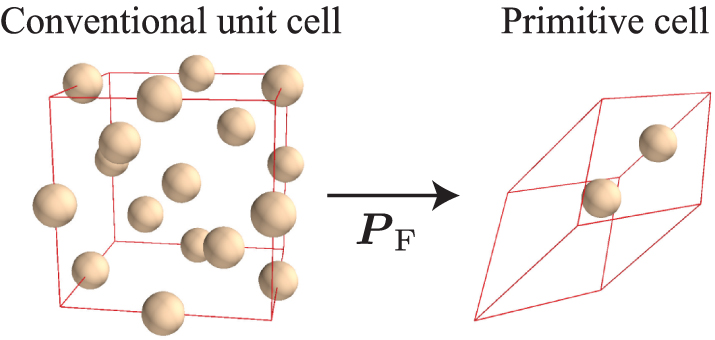
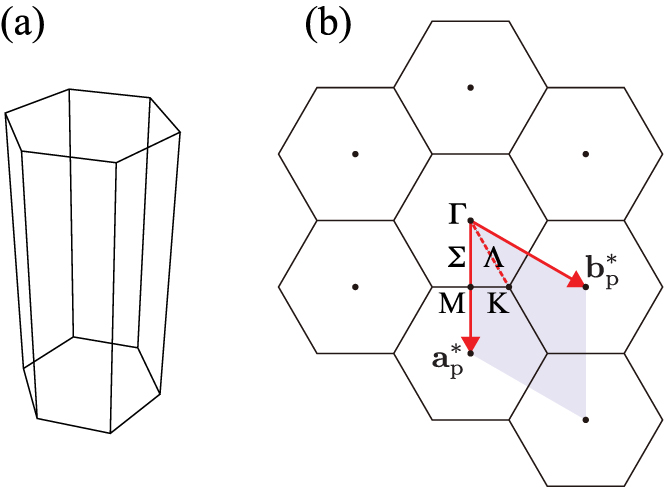
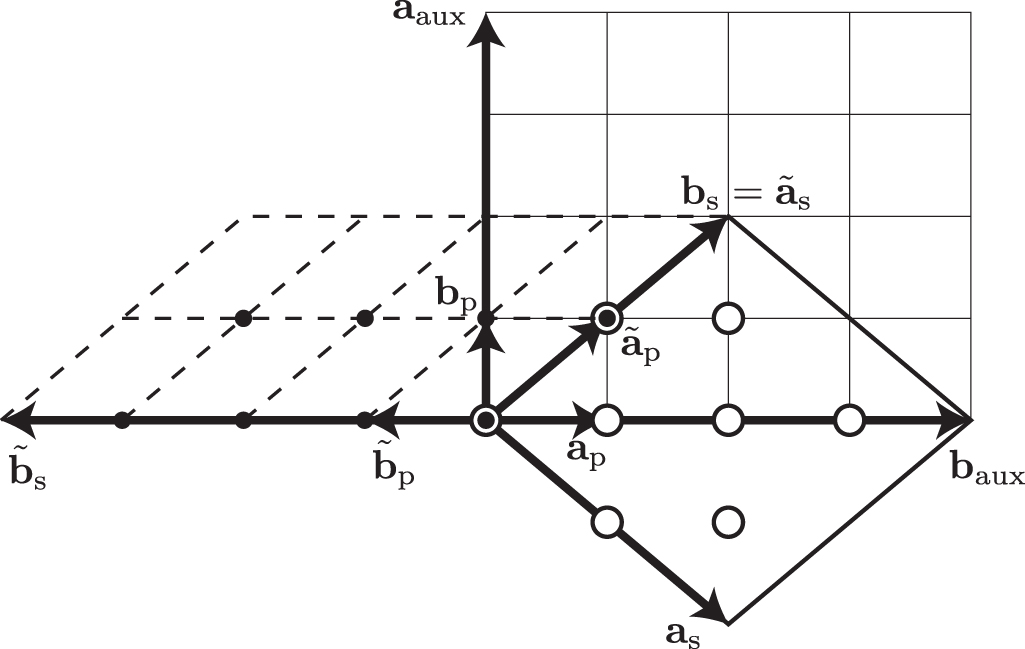
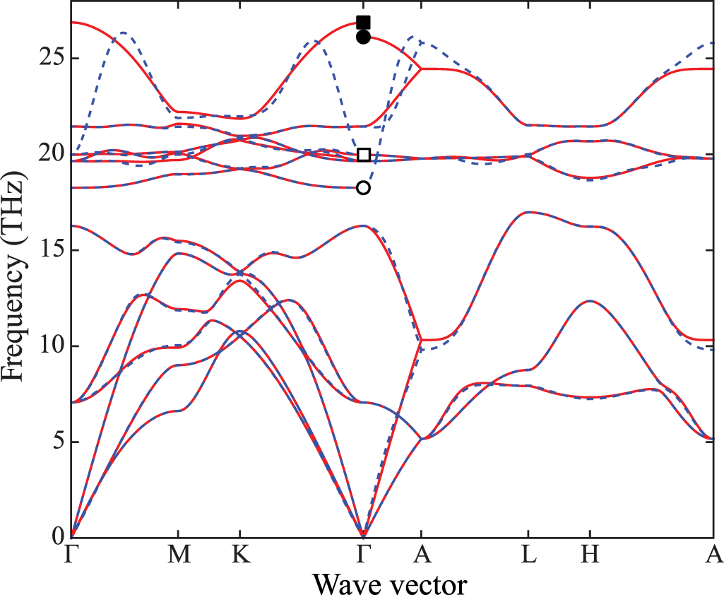
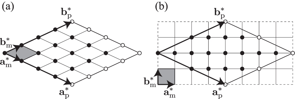
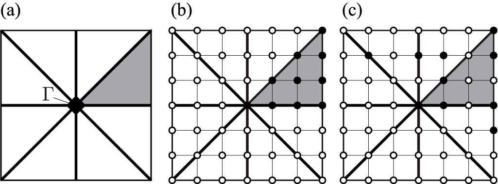
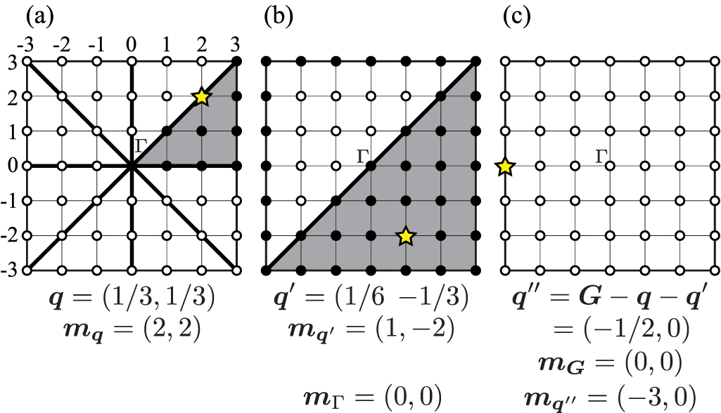
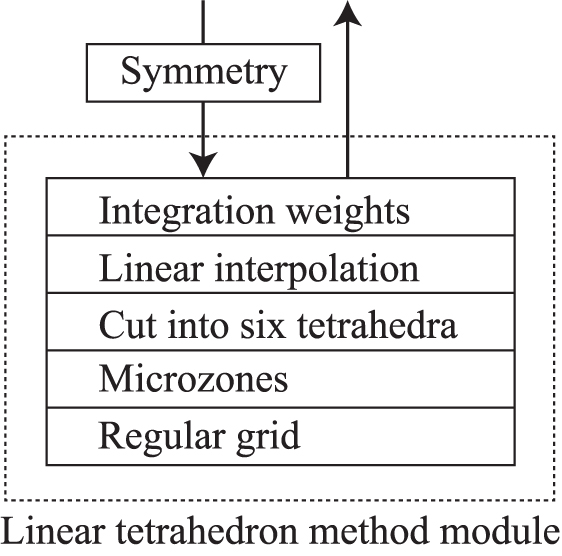
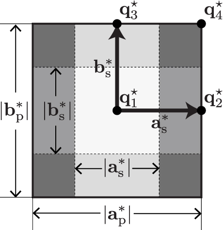
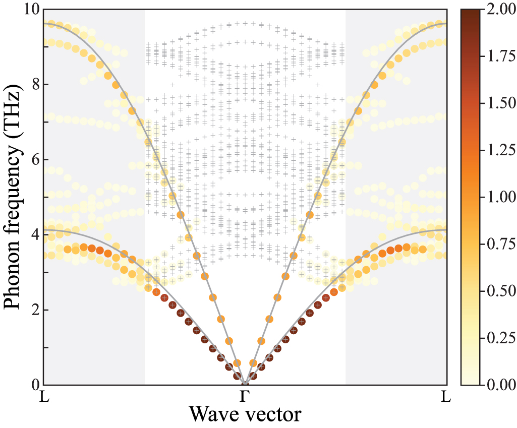
The tetrahedron is fully occupied, therefore,

$$\begin{align} g^i & = 0. \end{align} \tag{ A35 }$$

$$\begin{align} n^i & = 1. \end{align} \tag{ A36 }$$

$$\begin{align} I^{\,i}_k &= 0. \end{align} \tag{ A37 }$$

$$\begin{align} J^{\,i}_k &= 1/4. \end{align} \tag{ A38 }$$