

Abstract
Recent years have witnessed an ever growing interest in the interactions between hydrogen atoms and a graphene sheet. Largely motivated by the possibility of modulating the electric, optical and magnetic properties of graphene, a huge number of studies have appeared recently that added to and enlarged earlier investigations on graphite and other carbon materials. In this review we give a glimpse of the many facets of this adsorption process, as they emerged from these studies. The focus is on those issues that have been addressed in detail, under carefully controlled conditions, with an emphasis on the interplay between the adatom structures, their formation dynamics and the electric, magnetic and chemical properties of the carbon sheet.
Export citation and abstract BibTeX RIS
1. Introduction
The interaction between hydrogen atoms and graphite, and later graphene, has attracted ever increasing attention in the last two decades because of its relevance in such disparate fields as astrophysics, nuclear fusion, hydrogen storage and, not least, carbon-based and graphene technology.
The field has a long and curious history, with declines and renaissances. The first birth dates back long ago, in 1969, when Beitel used hydrogen on a graphite surface to test a new ultra-high vacuum apparatus (Beitel 1969). For decades, though, Beitel's work was ignored and the field remained essentially unexplored because of the widespread belief that hydrogen could not (chemically) adsorb on graphite. The system became object of extensive and detailed studies much later, in the 2000s. At the time the interest was mainly triggered by the astrochemical speculations about the role of carbonaceous surfaces in the formation of hydrogen molecules in space (Tielens 2013). Such problem is of great fundamental interest, since molecular hydrogen is by far the most abundant molecular species in the Universe and its formation mechanisms need to be known in detail in order to set up reliable astrophysical models for star and galaxy structure formation. Observations set stringent constraints on the possible species present on the surface of the dust grains that are found in the space between stars, and puzzling issues soon arose that stimulated an intense research activity in the field. The aim was to determine the energetics of the adsorbed species and to elucidate the sticking dynamics of the atoms impinging on the surface, as well as the pathways leading to molecular hydrogen formation. In this first stage, the focus was on graphite rather than on graphene but, in practice, most of the theoretical simulations adopted graphene as a computationally convenient model system.
This period marked the construction of a reliable single atom adsorption model and a first assessment of the ensuing surface chemistry, but it also witnessed a first decline of the interest in the field. It indeed became apparent that the ideal (0 0 0 1) surface of graphite was probably an oversimplified model for the surface of a carbonaceous dust grain, and that progress could only be made with further efforts aimed, e.g. at unveiling the influence of defects and morphology in the surface chemistry. Such issues were well beyond the aims of these early stage investigations, with so little experimental support that appeared of rather speculative nature.
With the isolation of graphene (Novoselov 2004) the field gained a new twist, and the study of the interaction between hydrogen and graphitic substrates received entirely new stimuli from the prospect of the many applications that may result when modulating the electronic and magnetic properties of this extraordinary material. In fact, chemical functionalization is one of the most successful ways to tune graphene electronic properties, and hydrogen is by far the adsorbate most widely used for this purpose. The influence of adatoms on graphene electronic properties is so huge that the surface chemistry of graphene soon emerged as a novel paradigm in surface science. This was partly expected since graphene was the first 'all-surface' material, i.e. one in which the 'bulk' properties are surface properties. However, the intricate and delicate interplay between adatom arrangement and substrate electronic properties came really as a surprise, and only later this was understood to be a consequence of the special position that graphene occupies in material science. In a sense, being it at the border between metals and insulators, it indeed inherits properties from both sides.
In this topical review we give a concise but comprehensive introduction to the extensive body of results, from both theory and experiments, that emerged over the years on various aspects involving hydrogen atoms on graphene. We shall proceed in order of increasing complexity. We first focus in section 2 on the diluted limit where the adatoms are essentially isolated on the surface, and only later move to more complex situations where dimers and clusters form on the surface (section 3). Additional issues such as the role of edges or other 'defects', as well as that of a supporting substrate, will be separately dealt with in subsequent sections (sections 4 and 5, respectively), where further (common) complications will be added to the previous background. Overall, we shall address energetic and dynamical issues involving the hydrogen atoms on the surface, but also the accompanying changes in graphene electronic structure and the interplay between electric, magnetic and chemical properties of the carbon sheet. The emphasis will be on key aspects that are well understood, although an attempt will also be made to single out issues that need further investigation, in the hope that this can stimulate further work on the subject.
We stress at the outset that while theoretical modeling is most often performed on graphene (either for computational convenience or for real interest into the substrate) the experimental information gathered so far under well controlled conditions only occasionally refer to graphene, either suspended or supported, and most often refers instead to graphite. With the due caveats, the latter translate with minor changes only to graphene. Hence, in the following, in absence of specific data for graphene, we shall use graphite as a model for graphene, i.e. in a sense, we shall view graphite as a graphene sheet laying on an inert (graphitic) substrate. It must be noted, though, that only 'graphene on graphite' can be considered effectively decoupled from the substrate (Li et al 2009), and thus interaction between layers should always be accounted for in a detailed comparison between theoretical results on graphene and experimental findings on graphite.
2. Low coverage
We start considering the adsorption properties in the diluted regime where H atoms can be considered quasi isolated. This is the ideal situation where to compare, at least in principle, theory and experiments in a detailed way. In practice, though, only a few experimental studies were able to address this regime, most of them employed higher coverages conditions where a rich behavior involving dimerization and clustering of adatoms is now known to occur. This has been confusing especially in the early days of activity in this field, when such richness of behavior was not fully appreciated and modeling of the adsorption process could only be partially successful in interpreting experimental results. The high coverage situation (for adatom concentrations just larger than about 0.01 per C atom) has to be considered separately and will be addressed in section 3. This need does not arise because of an interaction between adatoms that can either control the adsorption energetics or make their diffusive motion correlated. Rather, it is a consequence of the effects that adsorption has on the electronic structure of graphene, and that in turn affects reactivity, hence the adsorption kinetics. This feature is a rather striking property of graphene (and graphitic substrates in general) that has no analogues on other susbtrates (either metallic or semiconducting) commonly used in surface science.
2.1. Adsorption energetics
To set the stage of the present discussion we consider in this section the adsorption energetics in the diluted limit, addressing first the physisorbed regime and then moving to the more interesting chemisorbed one.
2.1.1. Physisorption.
Physisorption of hydrogen atoms on graphene and graphitic surfaces in general has long been considered a possible route for hydrogen storage. However, the depth of the physisorption well on clean surfaces is so small that no reliable storage device could be devised for operating at useful temperatures when only physisorbed species are considered (Tozzini and Pellegrini 2013). The problem remains of some interest for the chemistry of the interstellar clouds where formation of H2 molecules on the interstellar grains may occur on low temperature surfaces where physisorbed species are stable (e.g.  –20 K in the so-called diffuse clouds). At temperatures higher than
  K the rate of desorption is so large that refreshment of the surface is completed in a time-scale that is too short for astronomical standards.
The interaction potential relevant for this regime was characterized long ago by Ghio et al (1980) who used low energy H atom beams (50–65 meV) and first observed diffraction in the flux of scattered atoms off a graphite sample. They further measured a reduction of intensity in the specular reflection peaks, which was ascribed to the so-called selective adsorption, a kind of Feshbach resonance where the energy is temporarily channeled into closed diffraction channels. This confirmed the existence of an attractive interaction and suggested the presence of a reasonably deep adsorption well. From the position of the resonances Ghio et al estimated the well depth to be 43.3 ± 0.5 meV for graphite, and extrapolated this value to a single graphene layer to obtain 39.2 ± 0.5 meV (Ghio et al 1980).
Theoretical studies soon agreed in the position of the minimum being at the hollow site (i.e. at the center of a benzene ring) but the binding energies extracted from density functional theory (DFT) calculations were not sufficiently accurate because of well-known problems of DFT in handling dispersion forces. As a consequence, values in the range 0–100 meV were reported, despite the attempts of empirically correcting for van der Waals (vdW) interactions (see e.g. Ma et al (2011) and references therein). Good agreement between theory and experiment was achieved with the help of traditional quantum chemistry methods—second order, Møller–Plesset perturbation—on a cluster model (coronene, C24H12), using a rather large atomic basis-set and carefully correcting for the basis-set superposition error (BSSE) (Bonfanti et al 2007). This is essential to avoid sizable (unphysical) overbinding when weak interactions are of concern and geometry-dependent basis-sets are used. The H physisorption minimum was found at 2.93 Å above the surface plane with a depth of 39.7 meV at the hollow site, which decreases by only a few meV away from that site, thereby indicating a very small surface corrugation.
The findings of Bonfanti et al (2007) were confirmed by diffusion Monte Carlo studies on the same cluster model, although the same method applied to periodic graphene gave doubtful results (Ma et al 2011). Accurate parametrization of the empirical vdW correction was shown to give the required accuracy (Ferullo et al 2010) and, more recently, similar findings were obtained with the help of non-empirical, vdW-inclusive functionals (Bonfanti and Martinazzo 2018). These recent results pave the way for simulating H atom physisorption, diffusion and reactions with first principles means in a periodic setting, while accounting for the elusive vdW interactions in a reliable way.
2.1.2. Chemisorption.
Compared to several other surfaces, investigation of chemisorption of H atoms on graphitic substrates has started only recently (say the last 15 years), largely triggered by the raise of graphene. For some time, H atoms were not believed to be able to bind to the substrate, and early attempts to model the adsorption process without relaxing the surface failed in finding a chemisorption minimum. If fact, H atoms bind to the lattice only if (substantial) surface reconstruction is allowed, as first showed by Jeloiaca and Sidis on a cluster model (Jeloaica and Sidis 1999) and then by Sha and Jackson on a periodic setting (Sha and Jackson 2002). The authors of these studies found a binding energy  –0.65 eV, that was later refined with more converged calculations employing larger supercells. The value of the binding energy shows a sizable variability in the literature that can be ascribed to differences in the adopted DFT functionals and, more importantly, to the computational setup and the optimization strategy employed in the calculations. Accurate plane-waves DFT results unambiguously converge towards the value of
  0.85 eV, (0.85 eV in a 4 × 4 supercell (Hornekær et al 2006a), 0.84 eV in a 5 × 5 supercell (Casolo et al 2009a) and 0.87 eV in a 8 × 8 supercell (Lehtinen et al 2004)) while atomic-orbital based DFT results suggest a larger value (Ivanovskaya et al 2010) of 0.97 eV, likely because of the BSSE and the optimization strategy employed5. As for the length of the bond formed upon adsorption this is found typical of a CH in a hydrocarbon (∼1 Å), while the precise geometry of the deformed graphene structure remains sensitive to computational parameters (see table I in Casolo et al (2009a)).
2.1.3. Surface puckering.
The binding energy quoted above is of course much larger than the physisorbed one but remains rather small when compared to the interaction energy of H atoms on typical transition metal surfaces (∼2–2.5 eV) and to the CH bond energies in hydrocarbons (∼4 eV). The main reason for this discrepancy is that in forming a CH σ bond on graphene a considerable fraction of energy goes into the lattice, where it is stored indefinitely as deformation energy of the reconstructed (puckered) surface until the H atom is abstracted or desorbed, as we shall later when considering recombination of the adatoms to form H2.
Such a surface reconstruction consists in a 0.3–0.4 Å out of plane displacement of the binding carbon atom, and occurs as a consequence of a sp2–sp3 re-hybridization of the valence C orbitals that is needed to form the CH bond. The re-hybridization induces a change in the geometry of the substrate site, from a planar (sp2) to a tetrahedral (sp3) form, thereby 'puckering' the surface plane, a distortion which actually extends for tens of Angstroms away from the adsorption site (see figure 1). This is also evident in the energy landscape of figure 2 which shows the energy as a function of the heights of both the H and the binding C atom, for a collinear configuration of the two atoms (the remaining degrees of freedom being left to relax): the deep chemisorbed well is found at a non-zero height of the carbon atom above the surface, and can thus be reached only if the C atom pulls out from the graphene plane.
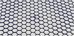
Figure 1. Equilibrium structure of a hydrogen monomer on graphene (balls and sticks) superimposed on a flat graphene structure (blue net) to highlight the short- and long-range details of the surface puckering accompanying adsorption. Results from large-scale DFT calculations using a rectangular unit cell of dimensions 4.7 × 3.4 nm2 (Achilli and Martinazzo 2018).
Download figure:
Standard image High-resolution image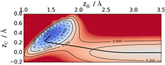
Figure 2. The potential energy surface of H on graphene as a function of the height of the atom on the surface zH and the perpendicular displacement of the binding carbon atom, zC. The black line is the minimum energy path. See main text for details.
Download figure:
Standard image High-resolution imageInterestingly, the lattice distortion accompanying hydrogen chemisorption impacts also on the electronic properties of graphene. It greatly enhances the otherwise negligible spin–orbit coupling (Castro Neto et al 2009, Zhou et al 2010), and makes possible the realization of the spin Hall effect (Balakrishnan et al 2013).
2.1.4. Sticking barrier.
Orbital re-hybridization is also responsible for an adsorption barrier ∼0.2 eV high, as it is made evident in figure 2 where this barrier is seen to separate the chemisorbed region from the physisorbed one. Such barrier prevents direct H atom adsorption unless high-energy beams are employed, and allows physisorbed atoms to desorb rather than converting into stable chemisorbed species.
Neumann et al (1992) were among the first to realize the need of hyperthermal beams ( K) for depositing H atoms on natural graphite6. With the help of x-ray photoelectron spectroscopy (XPS) they unambiguously proved adsorption of H atoms on graphite with formation of a strong C-H bond. Further detailed information on hydrogen chemisorption were later provided by Zecho et al (2002a) when exposing highly oriented pyrolytic graphite (HOPG) to a high-flux hyperthermal beam (
 K) of H(D) atoms, and using thermal desorption (TD) and high-resolution electron energy loss spectroscopy to investigate the species deposited on the surface at low temperature (
 K). Puzzling at that time was the double peak structure in their TD spectra (Zecho et al 2002a) and the absence of any peak around
  K where desorption was expected according to the binding energy ∼0.65 eV computed at that time. It took some years before dimer formation and recombination (Hornekær et al 2006a, 2006b) got uncovered and recognized to play a major role in the adsorption process (section 3).
From a theoretical perspective the barrier has been shown to arise from an avoided crossing between two diabatic electronic states, one purely repulsive in which the substrate electrons keep their ground-state coupling, and one strongly attractive describing the coupling between the H atom and a spin-excited electronic state of the substrate with two unpaired electrons (Casolo et al 2009a). The height of this barrier is yet unknown with precision, though results from standard DFT-GGA calculations cluster around 0.2 eV (Jeloaica and Sidis 1999, Sha and Jackson 2002, Ferro et al 2002, Hornekær et al 2006b, Casolo et al 2009a), a value that has been long considered a reasonable estimate. However, recent works employing vdW-inclusive DFT calculations claimed that the barrier height should be much smaller, if not vanishing (Moaied et al 2014, 2015, Brihuega and Yndurain 2018). Care is needed, though, in employing DFT for vdW interactions, especially in conjunction with atomic-like orbitals, because the combination of a (typically) overbinding functional with the ubiquitous BSSE may lead to errors of 0.2–0.3 eV that evidently wash out any adsorption barrier (Bonfanti and Martinazzo 2018). In addition, we mention that local and semilocal DFT functionals typically overestimate (underestimate) the binding (barrier) energies, particularly when the formation of true (i.e. directional) chemical bonds is involved, as it is the case for hydrogen on graphene. Coupled-cluster calculations on the coronene cluster model indeed found the barrier to be 370 meV, in reasonable agreement with previous multi-configuration quasi-degenerate perturbation theory results (Bonfanti et al 2011b). This estimate compares reasonably well only with the results of the accurate meta-hybrid functional M062X applied to the same system (328 meV), and it is considerable larger than the value obtained with the popular hybrid-functional B3LYP (262 meV) (Jensen et al 2018). Increasing the cluster size to circumcoronene (C54H18) decreases the barrier height to 304 (240) meV at the M062X (B3LYP) level, but it seems unlikely that its value attains ∼0.2 eV when extrapolated to the infinite size limit. Interestingly, the meta-semilocal functional M06L, that has been finding increasing interest in the condensed matter community, provides even larger estimates for the barrier, 407 meV for coronene and 390 meV for circumcoronene (Jensen et al 2018).
From the experimental point of view, the height of the adsorption barrier is yet unknown, but its existence is undeniable. Without an energy barrier for adsorbing H atoms, cold atomic beams would be effective in depositing H atoms on a room temperature surface, something that has been ruled out with dedicated experiments using an inductively coupled plasma source delivering 0.025 eV H atoms (Aréou et al 2011). In addition, a barrierless adsorption would make hydrogen deposition a completely random process, with an estimated abundance of dimers (and larger clusters) much smaller than that observed experimentally. Rather, the existence of the barrier and its sensitivity to changes in the electronic structure of the substrate make the formation of certain adspecies configurations more likely than others, as we shall see in detail below, in section 3.
In closing this section we notice that chemisorption could be barrierless if C atoms were 'prepared' in a sp3 configuration, as it is partially the case in graphitic substrates that are keen to bend, e.g. crumpled single layer graphene, or that are already bent, e.g. carbon nanotubes. We shall discuss these issues below in section 5.
2.2. Sticking and vibrational relaxation
We are now ready to discuss the sticking dynamics of H atoms on graphene. In the physisorbed state, the hydrogen atom is characterized by a very weak coupling with the substrate, and this allows considerable simplification when simulating its quantum dynamics, because of the fast convergence of the close-coupling expansion of the H+surface wavefunction (Medina and Jackson 2008, Lepetit and Jackson 2011, Lepetit et al 2011). Sticking probabilities including surface corrugation have thus been computed by several quantum means and found to be a few percent only (<0.05) for energies in the range 0–25 meV, although enhanced (∼0.10) at collision energies close to the diffraction resonances (Medina and Jackson 2008, Lepetit et al 2011). They are further increased on supported or suspended graphene, with interesting consequences for nanoelectromechanical devices (Lepetit et al 2011). Temperature was found to increase sticking because of the increased surface corrugation, though, as expected, it drastically reduces the desorption times (20–50 ps when  K, (Lepetit et al 2011)). Unfortunately, only a few experimental studies were conducted under conditions—very cold surfaces and low energy beams—in which H atoms can only physisorb and remain stable on the surface (Creighan et al 2006, Islam et al 2007, Latimer et al 2008). For this reason, no experimental result is available for the H atom sticking coefficient at energies of a few meV.
In contrast, in the chemisorbed regime, the presence of an adsorption barrier and the stronger coupling with the surface play a primary role in determining the sticking probability. Most of the available theoretical investigations (Sha et al 2005, Kerwin et al 2006, Kerwin and Jackson 2008, Morisset and Allouche 2008, Morisset et al 2010) agree (qualitatively) on the classical, over-barrier regime where energy transfer to the substrate is the only limiting factor. Only a few of them addressed the problem in the interesting regime where tunneling plays a dominant role and, until recently, none of them considered tunneling in the presence of a true dissipative quantum bath (the surface). This has been long rather unpleasant since it was known that the tunneling probability depends sensitively on the strength of dissipative effects (Caldeira and Leggett 1981).
The main problems hindering such a study are, on the one hand, the 'dimensionality curse' of the explicit quantum dynamical methods and, on the other hand, the lack of reliable reduced dimensional, open-system descriptions (quantum master equations)7. Recent years have indeed witnessed a tremendous progress in alleviating the exponential scaling problem of (numerically exact) quantum approaches—particularly with the multi-configuration time-dependent Hartree (MCTDH) method (Meyer et al 1990, Beck et al 2000, Meyer et al 2009) and its recent multi-layer variant (Wang and Thoss 2003, Manthe 2008, Vendrell and Meyer 2011) (ML-MCTDH)—but limitations remain in the form of the Hamiltonian terms that such methods can efficiently handle. Hence, a key step for investigating H sticking in the quantum regime was the formulation of a reliable model for chemisorption satisfying these constraints. This has been accomplished by some of the present authors (Bonfanti et al 2015a) using a system-bath strategy that is based on the reliability of a (generalized) Langevin description of the C atom dynamics. With such an assumption, the substrate has been mapped into a surrogate bath of independent oscillators, and the high-dimensional dynamical problem could be tackled with the MCTDH method in a numerically exact way (Bonfanti et al 2015b).
2.2.1. Vibration-phonon coupling.
As mentioned above, a crucial step to investigate sticking of H atoms on graphene at energies comparable to or smaller than the barrier height, is to devise a tractable yet reliable model Hamiltonian describing dissipation into the lattice. This is possible upon exploiting the effective equivalence between the (generalized) Langevin dynamics and the Hamiltonian dynamics of a properly designed 'independent oscillator' (IO) model (Weiss 2008). For H sticking on graphene, the key assumption (that can be checked a posteriori, see for instance figure 3, left panel) is that the dynamics of the binding C atom can be described by a generalized Langevin equation (GLE),
while the H atom is left to interact with C via an accurate (first principles) interaction potential  . In the above equation zC is the height of the binding C (the degree of freedom most relevant for sticking), mC its mass and
  is the position vector of the H atom. Furthermore,
  is understood to be a (causal) memory kernel and
  is a zero-mean Gaussian stochastic process related to
  by a fluctuation-dissipation theorem of the second kind,
 ![$ \renewcommand{\bra}[1]{\langle#1|} \renewcommand{\braket}[1]{\langle#1\rangle} \braket{\xi(t)\xi(0)}=\gamma(|t|)k_{B}T/m$](https://content.cld.iop.org/journals/0953-8984/30/28/283002/revision2/cmaac89fieqn019.gif) . As consequence, the GLE above is entirely determined by the memory friction
. As consequence, the GLE above is entirely determined by the memory friction  or, equivalently, by the so-called spectral density of the environmental coupling
  , that is defined to be
  , where
  is the Fourier transform of
  (Weiss 2008). Such spectral density turns out to be a key quantity for the non-Markovian Brownian dynamics of the GLE (Martinazzo et al 2011a, 2011b); in the present problem it can be understood as a phonon density of states on the binding carbon weighted by the coupling with the rest of the lattice.

Figure 3. Sticking probability as a function of the collision energy. Left: classical results for a fully atomistic potential and its surrogate IO model, at  K (green and blue curves, respectively) and
  K (red, magenta). Right: full quantum results at
  K (black line) alongside the classical results at
  K (green line). Also shown are the results of the impulsive model described in the main text (dashed lines).
Download figure:
Standard image High-resolution imageEquation (1) (and the accompanying equation for  ) is clearly of classical nature. However, the above mentioned equivalence with an IO Hamiltonian dynamics makes it a valid starting point for designing a quantum Hamiltonian that governs the (dissipative) quantum dynamics of interest. For the present problem such Hamiltonian takes the form
and describes a hydrogen atom interacting with the binding carbon that, in turn, interacts with a set of oscillators mimicking the rest of lattice. Crucial for this description is the size of bath8 and the choice of the harmonic oscillator frequencies ( ) and coupling coefficients (ck). The latter are required to 'sample' the spectral density of the GLE, and are typically chosen according to a uniform frequency spacing, even though optimal sampling scheme can be easily devised (Martinazzo et al 2011b).
In turn, a successful modeling requires that the spectral density is derived from the atomistic description, and this can be accomplished with the help of classical, molecular dynamics simulations. In our work (Bonfanti et al 2015a) the starting point was the equilibrium autocorrelation function for the hydrogen displacement (or velocity) during its oscillatory motion in the chemisorbed state, since such information is in principle experimentally available through several vibrational spectroscopies. Furthermore, such choice does not require any a priori knowledge of the system potential (Bonfanti et al 2015a, 2015c, Bonfanti and Martinazzo 2016b, Gottwald et al 2016), hence suits well to an ab initio molecular dynamics (AIMD) approach. The resulting model, though derived from an equilibrium situation, proved to be robust enough to accurately describe the non-equilibrium sticking dynamics up to collision energies well above the height of the barrier (Bonfanti et al 2015b). This is shown in figure 3 (left panel) where the classical results obtained with the atomistic potential are compared with those obtained with the IO model.
The IO model of equation (2) was first used to study the vibrational relaxation of a H atom chemisorbed on graphene (Bonfanti et al 2015a). It was found that the surface mode describing block oscillations of the CH unit above the surface relaxes quickly, in few tens of fs, because its frequency (∼470 cm−1) lies well below the Debye cutoff of the substrate. On the contrary, the H stretching mode (∼2550 cm−1 at the PBE level, 2650 cm−1 in the experiments, (Zecho et al 2002a)) lies above the Debye cutoff and thus its relaxation was found to be incomplete in the 3 ps-wide time window allowed by the chosen bath size (Bonfanti et al 2015a). Its lifetime was estimated to be ∼5 ps, a value that is incidentally very close to the value of 5.2 ps obtained by Sakong and Kratzer applying Fermi's golden rule in a first principles setting (Sakong and Kratzer 2010), i.e. a more appropriate and accurate method for this weak-coupling regime.
2.2.2. Sticking dynamics.
The results of the quantum dynamical calculations (Bonfanti et al 2015b) are reported in figure 3, which shows the sticking coefficient for both the classical and the quantum case, as obtained in the limiting case in which the H atom impinges on top of the binding C (only for a  K surface in the quantum case). Similar results have been recently obtained upon lifting the collinear assumption (Bonfanti et al 2018), apart for the size of the sticking probability that is approximately halved compared to the one in figure 3. In either cases it is found, as expected, that barrier-crossing plays the primary role at low collision energies, thereby allowing trapping into the chemisorption well for any projectile that is able to overcome the barrier. At high collision energies, however, energy transfer to the surface becomes the limiting factor, and fast H atoms hardly dissipate their excess energy and stick on the surface. As a consequence, the sticking coefficient attains a maximum at an energy which is about one and half larger than the barrier height.
Interestingly, it is further found that tunneling plays an important role only at energies much smaller than the barrier height. Rather, it is the zero-point motion of the binding carbon atom (i.e. the quantum fluctuations of the lattice) that plays a major role in determining sticking of the projectile H atoms, and makes a classical description of the process inadequate unless care is used to handle the zero-point energy issue. This is reasonable since, as figure 2 clearly shows, the motion of the C atom is strongly coupled to the 'sticking coordinate', and any tiny increase of its height above the surface determines a large decrease of the effective barrier to stick. This finding translates also in a marked dependence of the sticking probability on the surface temperature, but only in a classical setting: in the true, quantum setting the large Debye temperature of the surface leaves the lattice in the quantum regime for a wide temperature range.
As a matter of fact it was found that a simple impulsive model describing the collision of a classical projectile with a quantum surface reproduced the quantum results remarkably well for all but the lowest energies, thereby capturing the essential physics of such activated sticking dynamics, see right panel of figure 3 (Bonfanti et al 2015a, Bonfanti and Martinazzo 2016a). In this model, the energy available to the projectile for overcoming the barrier in the relative CH coordinate is the kinetic energy of H relative to C, and this is determined by both the collision energy Ecoll and the thermal agitation of the binding surface atom. For the projectile atom to cross the barrier (assuming that it travels leftward towards C) the carbon atom speed vC needs to exceed a threshold value  , where
  and
and  ,
,  being the projectile-target mass ratio and Eb the barrier height.
Once the atom has crossed the barrier, it is accelerated by the attractive interaction with the surface atom and energy transfer takes place to an extent that is determined by vC, hence by the surface temperature Ts. The precise amount of energy that is transferred to the surface can be computed in the impulsive limit, which is appropriate at the high collision energies where energy dissipation dominates. Under these conditions, trapping occurs only when vC lies in a specific interval
where  ,
,  and D is an 'effective' depth for the interaction well. Hence, if this hard-collision limit kept down to low energies, the sticking probability would follow from integrating the distribution of the carbon atom velocities over the interval
  , i.e.
where  is the velocity distribution appropriate to the C atom. Tunneling corrections are also possible at this stage by removing the threshold on vC and introducing the appropriate tunneling probability in the integral, and this proved to improve the accuracy of the model down to the lowest energy considered (Bonfanti et al 2018).
Crucial for the success of the model is the choice of  , since the classical (Maxwell–Bolztmann) velocity distribution proved to be inadequate to reproduce the quantum results. Rather, one needs the velocity distribution of the carbon atom quantum oscillator, which depends on both its fundamental frequency and on the coupling with the rest of the lattice. Since vC is a linear combination of Gaussian variables (the normal modes of the substrate) the required function
  is readily seen to take a Gaussian form similar to that of an independent oscillator (Bonfanti et al 2015b),
but with a temperature-dependent effective frequency  that accounts for the coupling to the bath. Only in the high temperature limit (in fact, for
  , where TD is the Debye temperature,
  K in graphene)
  increases linearly with Ts and
  in equation (5) takes the standard form of a Maxwell–Boltzmann distribution.
The computed 'initial' sticking co-efficient has been recently used in a simple kinetic model devised to understand the adsorption process of H atoms on graphene at low coverages (Bonfanti et al 2018). The model included only sticking, dimer formation and Eley–Rideal reactions, and was found to describe rather well the hydrogen uptake curves measured long ago by Beitel on graphite (Beitel 1969) and more recently by Haberer and coworkers on graphene on gold (Haberer et al 2011a, 2011b). It also helped to rationalize the isotopic effect observed by Paris et al (2013) but, unexpectedly, was found somewhat at odds with the findings on HOPG (Zecho et al 2002a, Andree et al 2006). The reason of this discrepancy might lie in the fact that HOPG is of high-quality form only from a crystallographic point of view, and its defect concentration might have a pronounced effect on the macroscopic adsorption process.
2.3. Mobility and diffusion
We have seen in section 2.1 that the weak physisorption well is only slightly corrugated. Indeed, the lowest energy diffusion barrier is only 4 meV, and physisorbed hydrogen atoms are very mobile even at vanishing temperatures due to tunneling (Bonfanti et al 2007). Wavepacket calculations have been used to estimate the site-to-site 'hopping' and found that it occurs on a 1 ps time-scale, corresponding to a huge value of the  K limiting diffusion coefficient, 1.7 × 10⁻⁴ cm2 s−1. In other words, physisorbed H atoms do not stay at rest in their equilibrium position even in the absence of thermal fluctuations.
On the contrary, chemisorbed hydrogen atoms are rather immobile on the surface. This is a consequence of the nature of the carbon–hydrogen bond—i.e. a true, covalent chemical bond—that requires it to be completely broken before the H atom can move to another site. In other words, the barrier to diffusion matches the desorption barrier, in a way that chemisorbed H atom desorb rather than diffuse. Indeed, prolonged observations of hydrogen monomers at  K with STM showed that H (D) atoms are immobile at any coverage (Hornekær et al 2006a). Calculations predict a diffusion barrier of ∼1.1 eV, i.e., larger than the desorption barrier.
The situation changes drastically under charge doping (Huang et al 2011). Electron doping heightens the diffusion potential barrier, but hole doping lowers it, thereby making H atom diffusion possible on the surface. Desorption, on the other hand, is made more difficult by both kinds of doping, as they increase the chemisorption binding energy much more than they decrease the adsorption barrier. The reason is that electrons (holes) populate the antibonding (bonding) orbitals of the  (π) bands, and thus weaken the π bonds in graphene, increasing the chemisorption energy. This effect becomes beneficial for diffusion under hole doping because the relevant transition state involves a partially positively charged H atom that gets stabilized by a positively charged substrate.
2.4. Reaction
Formation of hydrogen molecules from hydrogen atoms adsorbed on the graphene surface is a likely outcome since the reaction exothermicity makes the reaction thermodynamically favored and the absence of barrier (in any of the possible routes to the molecular product) renders it kinetically possible in a wide range of conditions. The formation reaction, often termed 'recombination' with reference to the thermodynamically stable form that hydrogen takes in the gas-phase, frees a huge amount of energy that mainly goes into the product molecule though, as we shall see below, a considerable fraction can be left on the lattice when at least one of the recombining hydrogen atoms is chemisorbed on the surface. It is important to establish the correct energy partitioning because this impacts, for instance, both the surface and the gas-phase chemistry of the interstellar medium (Tielens 2013).
As common in surface chemistry, H2 recombination on graphene can occur through three different basic mechanisms: Langmuir–Hinshelwood (LH), Eley–Rideal (ER) and hot-atom (HA). In the LH mechanism, both reactants are adsorbed on the substrate and diffuse until they meet each other and react. The ER mechanism occurs when only one of the reactant adsorbs onto the surface, the second comes directly from the gas phase and forms the product molecule in a direct collision. Finally, the HA process is intermediate, since one of the reactants is trapped on the surface but not equilibrated, and typically diffuses hyperthermally until it encounters the reaction partner. In the following, we discuss the relevance of these mechanism on graphene, depending on the physical conditions considered.
2.4.1. Langmuir–Hinshelwood, hot-atom and Eley–Rideal.
For hydrogen recombination on graphene LH is relevant in the physisorbed regime only since, as shown above, chemisorbed atoms prefer to desorb rather than diffusing. Even in this case, however, LH is not really standard, since thermalization of the physisorbed species in stable adsorption sites (as required by the reaction mechanism) is hampered by zero-point fluctuations. The reaction efficiency for two atoms trapped on the surface and approaching each other has been studied with wave packet techniques (Morisset et al 2004a, 2005), and found very high. The reaction should occur through the deflection of the two projectiles toward and away from the surface plane: the rebound of the first transfers energy to the nascent molecule giving rise to a strong rotational excitation. Then, molecular hydrogen either desorbs immediately or stays trapped on the surface in a metastable state, and it is vibrationally hot, and rotationally highly excited (Morisset et al 2004a, 2005).
The relevance of HA recombination for hydrogen on graphene is yet unclear, for it requires a weakly corrugated but rather strong atom–surface interaction that can trap hyperthermal atoms and prevent them to desorb during their excursion along the surface. HA is probably operative when H atoms trap in the physisorbed well of well-cleaned surfaces, but it is expected to be rather sensitive to the surface temperature because of the huge effect that the latter has on the hot-atom lifetime. In addition, formation of hot-atoms from gas-phase projectiles requires a source of corrugation (such as, e.g. that provided by an adsorbed species) that can channel energy from the beam direction (typically normal to the surface) to the surface plane. Nevertheless, there are evidences that HA reaction occurred, in conjunction with ER abstraction, in the experiments by Zecho et al on HOPG (Zecho et al 2002b), since the extracted 'effective' abstraction cross-sections (>16  at
at  K) were found to decrease with increasing surface temperature and to level off at high temperature (∼3.5
  ) (Zecho 2007). These results suggest that hot-atoms might play an important role when the temperature is sufficiently low (and the surface sufficiently clean) that such fast-moving atoms stay on the surface long enough to encounter a reaction partner.
One comment is in order in this context since the same abstraction experiments (Zecho et al 2002a) were found to agree rather well with the results of the first realistic quantum calculations of the ER cross-section (Zecho et al 2002b). The agreement should be considered fortuitous since, on one hand, the theoretical results were not corrected for the 1/4 spin-statistical factor appropriate for this reaction (Casolo et al 2009b, 2013) (see also below) while, on the other hand, as argued above, the experimental ones likely accounted for HA reactions too. Comparison between the saturation value of the cross-section (∼3.5  ) and 1/4 of the theoretical estimate would give an agreement similar to that claimed in the original work (Zecho et al 2002b), which can be improved by accounting for the competing reaction channels (Casolo et al 2013).
The ER reaction, usually of secondary importance for different surfaces, becomes very important here for chemisorbed species, in the wide temperature range where the latter are stable on the surface and physisorbed species are not present (say for Ts in the range 50–300 K at low coverage, and Ts in the range 50–500 K at higher coverage, see section 3). As will be discussed in section 3.1.2, it generally competes with sticking (dimer formation) when the substrate is exposed to hot H atoms, and the 'branching ratio' depends markedly on the energy of the incoming H atoms. However, when cold atoms are used on a H pre-covered sample, abstraction dominates over dimer formation, as shown experimentally (Aréou et al 2011) and confirmed by theory (Casolo et al 2013).
This reaction mechanism has been extensively studied over the years, both theoretically and experimentally, mainly because of its importance for the interstellar chemistry (Tielens 2013). Several specific aspects of the dynamics have been addressed (the size of the cross sections, the internal excitation of the product molecules, the role of the collision energy and of the vibrational excitation of the adsorbate, the effect of isotopic substitutions, etc) upon resorting to various approximations, either in the dynamics or in the model (Jackson and Lemoine 2001, Meijer et al 2001, Farebrother et al 2002, Zecho et al 2002b, Sha et al 2002, Morisset et al 2003, 2004b, Martinazzo and Tantardini 2006a, 2006b, Casolo et al 2009b, Bachellerie et al 2009b, Sizun et al 2010, Pasquini et al 2016). Quantum dynamics was mostly restricted to the rigid, flat approximation (Sha et al 2002, Zecho et al 2002b, Martinazzo and Tantardini 2005, 2006a, Casolo et al 2009b), and the dynamics was addressed in two opposite limits, namely a reaction much faster than the surface atom motion ('diabatic' limit) or such slow that C fully relaxes during the projectile motion ('adiabatic' limit). These quantum studies all show a reaction cross-section that increase steadily with energy till the competing collision induced desorption (CID) channel opens up. In this regime, total reaction cross sections showed singular quantum oscillations that witnessed an unusual reaction mechanism leading to selective population of the low-lying H2 vibrational levels (Martinazzo and Tantardini 2005, 2006a). Extension to the cold collision energy regime  –10−2 eV (Casolo et al 2009b), on the other hand, showed that reaction could also be hampered by quantum reflection despite the absence of any barrier (Bonfanti et al 2011a). This quantum effect may indeed arise in the presence of deep and narrow potential wells whenever the projectile De Broglie's wavelength approaches the size of the well to be crossed.
Overall, general consensus has been reached on the large size of the cross-section and on the flow of a large fraction of the reaction exothermicity into product vibrational excitation. The strong H–H interaction dominates the dynamics, and product molecules can form and leave the surface as soon as the two hydrogen atoms get closer than about twice the equilibrium internuclear distance in H2 (∼0.7 Å). In addition, chemisorbed H atoms are relatively far from the surface and this allows steering of the projectile, with relatively large cross-section (∼10  when not yet corrected for the spin statistical factor). This is in sharp contrast with metal surfaces where stronger H–substrate interactions (and shorter equilibrium geometries) 'mask' the target atom to the hydrogen projectile and leads to much smaller cross-section (<1
  on metals).
For physisorbed targets the reaction was found to be very efficient down to 1 K (Martinazzo and Tantardini 2006b, Casolo et al 2009b). However, in this case the CID channel opens up at quite small energies (∼40 meV) and becomes soon very efficient, thereby causing a rapid drop of the reaction efficiency. A large cross-section for trapping H atom projectiles was predicted that might trigger HA reactions (Martinazzo and Tantardini 2006b, Casolo et al 2009b).
2.4.2. Product vibrational excitation.
As mentioned above, a striking feature of the H2 formation reactions on graphene and graphitic surfaces is the vibrational excitation of the product molecules. This is interesting for several reasons. In the chemistry of the interstellar clouds, for instance, the vibrational excitation of the H2 molecules triggers some endothermic reactions that would be otherwise prohibited by the severe conditions of the interstellar clouds, e.g. H2 + C+ → CH+ + H (Agúndez et al 2010, Bonfanti et al 2014). On the other hand, vibrationally hot molecules easily form negative ions by dissociative attachment, H2 + e− → H + H−. Thus, they provide a viable route to produce negative ion sources, to be used, for instance, in heating and current drive systems in experimental fusion reactors.
Theoretical calculations agree on the vibrational excitation of the product molecules, being them obtained from LH or ER, employing either chemisorbed or physisorbed species, although the precise level of excitation may differ from one study to the other because of details in the interaction potentials or in the adopted dynamical approach. Experiments employed cold HOPG surfaces ( –15 K) and cold beams (
 K), i.e. in a regime mostly relevant for LH recombination between physisorbed species, and used resonant enhanced multi photon ionization to probe the product energy (Latimer et al 2008). The rovibrational distributions of the nascent molecule were found to peak at the first few values of the rotational quantum number j and at much larger value of the vibrational quantum number
  . The observed low rotational excitation is at odds with theoretical predictions on LH/HA recombination of physisorbed species, since in the simulations H2 molecules were found with a much larger rotational excitation (Morisset et al 2004a, 2005, Bachellerie et al 2009a). They agree much better with those computed with ab initio molecular dynamics in an unrestricted investigation of the ER reaction involving chemisorbed species (Casolo et al 2013), thereby suggesting that chemisorbed H atoms might play also a role at the extreme conditions of the experiments (Latimer et al 2008), see figure 4 and section 3.1.2.
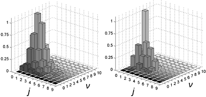
Figure 4. Comparison between experimental (Latimer et al 2008) (left panel) and theoretical (right panel) relative populations of HD formed in a recombination reaction on HOPG. Copyright Casolo et al 2013. National Academy of Sciences.
Download figure:
Standard image High-resolution image2.4.3. Substrate heating.
The dynamical role of the lattice, as well as its ability to absorb part of the reaction energy, has received little attention. Molecular dynamics (Bachellerie et al 2009a) and ab initio molecular dynamics (Casolo et al 2013, 2016) investigations did assess the role of the substrate but in a classical setting and with different aims, while, as mentioned above, quantum dynamical studies were mostly restricted to reduced dimensional models that completely neglected the dynamical role of the substrate or reduced it to that of the binding carbon only at the expense of other degrees of freedom.
Progress in this direction has been recently made by extending the model developed for the sticking dynamics (section 2.2) to account for the presence of an additional H atom (Pasquini et al 2018). Despite the limitation of a collinear approach, the mentioned study represents the first unrestricted investigation of the C atom dynamics (and its energy exchange with the rest of the lattice) during the reaction, in the correct quantum setting most appropriate for a light atom dynamics. Indeed, even though the reaction dynamics is reasonably well described by classical means at all but the lowest collision energies, lattice quantum fluctuations need to be correctly taken into account for a correct description of the reaction (see also section 2.2). One of the main findings of this study is that the C atom dynamics is essential for the reaction, while the rest of the lattice plays a secondary role only. The reason is that, even though unpuckering of the surface is fast—some tens of fs, in accordance with the short relaxation time found for the related CH surface mode, see section 2.2—it starts only after formation of H2 is completed. As a major consequence a considerable substrate heating occurs: the energy stored in the puckered surface is left entirely on the lattice, ∼0.8 eV per reactive event. Adding the energy that is necessarily dissipated when chemisorbing the first H atom (the 'target' in the ER abstraction) one finds that about 1.6 eV per H atom pair is stored in graphene. This result is in sharp contrast with the situation in which two physisorbed H atoms recombine via LH kinetics, in which case only (twice) the H atom physisorption energy is left on the surface.
It is worth noticing in this context that, although theoretical modeling was invariably performed in the (electronically) adiabatic approximation, it is likely that the large amount of chemical energy that is quickly released into the lattice triggers non-adiabatic effects and creates e–h pairs. In principle, such 'chemically induced' e–h pairs could be detected as chemi-currents (Gergen 2001, Nienhaus 2002, Kandratsenka et al 2018).
2.5. Midgap states
We now turn our attention to the effects that H atom adsorption has on the substrate electronic structure, since these proved to influence both the charge transport properties and the chemistry of graphene. Chemisorbed hydrogen atoms, similarly to many other species that covalently bind to the substrate (as well as to carbon atom vacancies), act by removing a pZ orbital from the π cloud, thereby affecting the electronic states at low energies because of the bipartite graphene's nature9. This is already evident upon counting the states and taking into account the e–h symmetry: removal of a single site results in a odd-numbered system that necessarily has a zero energy level ('zero energy mode'). This zero-energy state is a singly occupied molecular 'orbital' dubbed midgap state that localizes on the majority sublattice (see section 3.4). Real graphene is not exactly bipartite because of the hoppings beyond the nearest-neighbor ones, hence the 'zero' energy mode is not exactly at the Fermi level though it remains very close to it for reasonable values of the hopping energies.
First-principles calculations go beyond the tight-binding approximation and account, at least in principle, for the electron correlation. DFT results for a C atom vacancy and several adsorbed species (H, F, OH, CH3, etc) confirm this picture and show that, from an electronic point of view, such 'pZ vacancies' have a sort of universal behavior, with common features in the density of states, spatial appearance, chemical properties, etc. First principles results for a H adatom are reported in figure 5 for a rather large simulation cell, a rectangular unit cell of dimensions 4.7 × 3.4 nm2 containing more than 600 atoms (Achilli and Martinazzo 2018). There is seen that the spin-polarized density of states (DOS) has two peaks, one slightly below the Fermi level and one slightly above it, thereby describing a singly occupied level (left and middle panels in figure 5). Splitting (∼140 meV in figure 5) is due to Coloumb repulsion in such energy level and it is a measure of the spatial extension of the electronic state, which semilocalizes around the adatom occupying roughly the majority sublattice only. This is shown in figure 5 (right panel), and agrees well with the predictions of the imbalance rule and of simple models (see below).
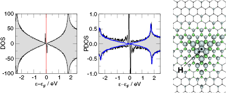
Figure 5. Density of states and spin-density for H chemisorbed on graphene (results of fully relaxed first principles calculations on a large supercell, corresponding to ∼10−3 H per C atom, (Achilli and Martinazzo 2018)). Left: total DOS for spin-up (positive values) and spin-down (negative values) channels. Middle: DOS projected onto a lattice site close to H (nearest-neighbor of the hydrogenated site, black curve), and far from it (blue). Right: ±0.004 
 isosurfaces of the ensuing spin-density.
Download figure:
Standard image High-resolution image2.5.1. Resonating valence bond picture.
From a chemical perspective midgap states arise naturally in the resonant valence bond (RVB) description of graphene once breaking a double bond and 'resonating'. Such a picture—though most often confined to a qualitative level—is a simple graphical translation of the RVB variational wavefunction which, for a singlet state, reads as
where  creates an electron in site i with spin σ, the product runs over all pairs (
 ) that define linearly independent 'spin-couplings' and cI's are variational parameters. In the above equation each pairing I represents a chemical structure and the superposition is commonly known as chemical resonance. Figure 6, for instance, shows two of the many graphene's chemical structures with
  indicating the above superposition. The number of independent couplings is a group-theoretical object that increases quickly with increasing the number of electrons10 and this prevents the use of the above ansatz for all but the simplest systems. However, limiting the pairs to the nearest neighbors ones (the so-called Kekulé structures) leads to considerable saving without seriously affecting the accuracy (Wu et al 2002, 2003) (coronene, for instance, with its 24 π electrons has 208,012 singlet couplings but only 20 Kekulé structures) and further saving is possible by recognizing that the largest contribution to the chemical resonance is provided by the Clar's formulas (Solà 2013), i.e. those structures that maximize the number of sextets (for coronene there exist only two of such Clar's formulas).

Figure 6. Some 'resonating' Kekulé structures for graphene (top row) and hydrogenated graphene (bottom row) showing the bond switching mechanism that sets free an unpaired electron in the majority sublattice.
Download figure:
Standard image High-resolution imageNow, considering H adsorption, it is not hard to realize that binding of a H atom breaks the aromatic network and leaves one unpaired electron on the lattice that is free to move by 'bond switching': spin re-coupling with a neighboring double bond creates an unpaired electron in one every two lattice sites, on the same majority set predicted by the counting rule mentioned above (figure 6, bottom). In fact, such itinerant electron is equivalently described by a singly occupied molecular orbital delocalized on such a set. As we shall see in the following, despite its simplicity, such picture is powerful in describing spin and/or charge density localization in π-conjugated molecules and in graphene, and proved to be rather useful for predicting chemical reactivity.
2.5.2. Density of states.
A quantitative look at the zero-energy modes in graphene is provided by the (noninteracting) Anderson model (Anderson 1961, Robinson et al 2008, Wehling et al 2010), which we discuss here in some detail because it is instrumental for the following section. In this model the ad-species is described by a single level at energy  (in our case the 1 s level of the H atom), which is let to hybridize with a carbon atom of the lattice, say of A type at the origin, by adding the term
to the lattice Hamiltonian
In these equations W is the hybridization energy, 
 creates (destroys) an electron with spin σ in the adatom energy level,
  (
( ) does the same for the lattice site i and t,
  are the hopping energies for the nearest-neighbors (NN) and next-nearest-neighbors pairs. The problem is best handled with the help of the Green's operator11
  of the one-electron Hamiltonian, upon partitioning the one-electron space into a primary subspace (the lattice) and the remainder (Levine 1969). In fact, it is not hard to show that the projection of the exact Green's operator onto the lattice takes the simple form12
  where
where  is an effective, energy-dependent Hamiltonian implicitly accounting for the dynamics in the adatom level, i.e.
  , where
  reads as
![$ \renewcommand{\ket}[1]{|#1\rangle} \ket{\chi_{0, \sigma}}$](https://content.cld.iop.org/journals/0953-8984/30/28/283002/revision2/cmaac89fieqn077.gif) being a pZ spin–orbital at site 0. It is thus seen that, as long as the electron dynamics in the lattice is of concern, hybridization with an impurity level introduces an energy dependent scattering potential
being a pZ spin–orbital at site 0. It is thus seen that, as long as the electron dynamics in the lattice is of concern, hybridization with an impurity level introduces an energy dependent scattering potential  that becomes strong for energies approaching the adatom level. A solution of this scattering problem is possible with the help of the T operator (Taylor 1969), here defined to be
  , since the corresponding Lippmann–Schwinger equation
  (where G0 is the Green's operator of the unperturbed lattice) is solved by
when the potential takes a separable form. In turn, knowledge of the T-matrix allows one to obtain the required lattice Green's operator as  and thus solve the scattering problem. In equation (6),
  is the on-site Green's function of the unperturbed lattice,
 ![$ \renewcommand{\bra}[1]{\langle#1|} \renewcommand{\braket}[1]{\langle#1\rangle} g_{00}^{0}=\braket{{\bf 0}\sigma|G^{0}(\lambda)|{\bf 0}\sigma}$](https://content.cld.iop.org/journals/0953-8984/30/28/283002/revision2/cmaac89fieqn083.gif) , which for graphene in the linear band approximation takes the form
, which for graphene in the linear band approximation takes the form
where  is the density of states per C atom per spin channel,
  . Here,
  is an energy cutoff that determines the bandwidth and that is inversely related to the carbon–carbon bond length dCC, i.e.
  (matching
  to the known low-energy expression for the density of states in graphene would result in
  or
or  eV). Notice that for
  , for any linear (and sublinear) density of states the real part of the on-site Green's function (
 ) features a vertical cusp that makes the position of the resonance in the T-matrix (i.e. the lowest energy solution of the equation
  ) rather insensitive to the hybridization energy W and always very close to
  .
.
With the  operator at hand, one readily obtains the density of states at the lattice sites,
  . The calculation is straightforward when the total density of states is of interest, since elementary algebra shows that it takes the form (per C atom, per spin channel)
where NC is the number of lattice sites (this expression contains also the contribution of the adatom level,  , as it turns out from the Green's operator projected in the secondary space,
  ). It is readily seen that
  when
when  , except for a positive peak
  wide around the adatom energy level when
  which becomes a sharp peak between
  and
and  when
when  . Wehling et al (2009) fitted ab initio results to tight binding models and found for hydrogen (and several other neutral species)
  eV and
  eV, thereby placing the resonance at a energy of about −0.06 eV, in agreement with the results of figure 5. In this context, it is worth noticing that both the adatom level and the binding C site contribute little to the density of states in this spectral window, since they form a bonding–antibonding pair of states which move far from the Fermi level. This becomes evident when
  since in such case the binding C and the adatom level give each a contribution of
 ![$ \newcommand{\e}{{\rm e}} \frac{1}{2}\left[\delta(\epsilon-W)+\delta(\epsilon+W)\right]$](https://content.cld.iop.org/journals/0953-8984/30/28/283002/revision2/cmaac89fieqn109.gif) which separates out from the band.
which separates out from the band.
2.5.3. Spatial properties.
Of great interest are also the spatial properties of the H-induced resonance which, as seen in figure 5, semilocalizes around the adatom and decays away from it with a characteristic power law. This behavior is also evident when imaging H atoms with STM, since a bright protusion around the adatom appears at small bias and displays a characteristic threefold symmetry (Wang et al 2006). In the T-matrix approach to the Anderson problem these properties can be investigated by looking at the scattered component ![$ \renewcommand{\ket}[1]{|#1\rangle} \newcommand{\e}{{\rm e}} \ket{\psi_{\epsilon}^{{\rm scatt}}}$](https://content.cld.iop.org/journals/0953-8984/30/28/283002/revision2/cmaac89fieqn110.gif) of the scattering state
of the scattering state ![$ \renewcommand{\ket}[1]{|#1\rangle} \newcommand{\e}{{\rm e}} \ket{\psi_{\epsilon}+}$](https://content.cld.iop.org/journals/0953-8984/30/28/283002/revision2/cmaac89fieqn111.gif) ,
,

where ![$ \renewcommand{\ket}[1]{|#1\rangle} \newcommand{\e}{{\rm e}} \ket{\psi_{\epsilon}^{0}}$](https://content.cld.iop.org/journals/0953-8984/30/28/283002/revision2/cmaac89fieqn112.gif) is an eigenstate of the unperturbed lattice with energy
is an eigenstate of the unperturbed lattice with energy  . It is clear that such scattering component requires computation of the off-site Green's function, being it proportional to
where ![$ \renewcommand{\bra}[1]{\langle#1|} \renewcommand{\braket}[1]{\langle#1\rangle} \newcommand{\e}{{\rm e}} G^{0}({\bf r}, {\bf 0}|\epsilon)=\braket{{\bf r}\sigma|G^{0}(\epsilon)|{\bf 0}\sigma}$](https://content.cld.iop.org/journals/0953-8984/30/28/283002/revision2/cmaac89fieqn113.gif) for a H adatom binding to the site at the origin (of A type in the following). This quantity has been considered by several authors for different reasons, ranging from investigations of STM imaging (Wang et al 2006) to Ruderman–Kittel–Kasuya–Yosida (RKKY) interactions in graphene (Sherafati and Satpathy 2011a, 2011b, Kogan 2011). It can be obtained numerically as Fourier transform of the (simpler) Green's function in k-space, namely from
for a H adatom binding to the site at the origin (of A type in the following). This quantity has been considered by several authors for different reasons, ranging from investigations of STM imaging (Wang et al 2006) to Ruderman–Kittel–Kasuya–Yosida (RKKY) interactions in graphene (Sherafati and Satpathy 2011a, 2011b, Kogan 2011). It can be obtained numerically as Fourier transform of the (simpler) Green's function in k-space, namely from
where  depending on whether
  is a lattice position in the A or B sublattice (
 and
and  , respectively, in the following), the integral runs over the Brillouin zone (BZ) and
  is its area. Here,
 ![$ \renewcommand{\bra}[1]{\langle#1|} \renewcommand{\braket}[1]{\langle#1\rangle} \newcommand{\e}{{\rm e}} G_{XY}^{0}({\bf k}|\epsilon)=\lim_{\eta\rightarrow0^{+}}\braket{\phi_{{\bf k}X}|(\epsilon+{\rm i}\eta-H_{{\bf k}}){}^{-1}|\phi_{{\bf k}Y}}$](https://content.cld.iop.org/journals/0953-8984/30/28/283002/revision2/cmaac89fieqn119.gif) , where
, where ![$ \renewcommand{\ket}[1]{|#1\rangle} \ket{\phi_{{\bf k}, X}}$](https://content.cld.iop.org/journals/0953-8984/30/28/283002/revision2/cmaac89fieqn120.gif) is a Bloch state built with
is a Bloch state built with  basis functions and
  is the k − Hamiltonian (for the above two-band model of graphene, a 2 × 2 matrix in the sublattice indexes). Fortunately, at the low energies of interest for the H-induced resonance, one can use the linear band approximation and expand the above integrand around the K, K' points, remove the energy cutoff
  with negligible error (for not too small distances,
  ) and perform the integral analytically. Following this route we find
where  are Hankel functions of the first and second kind (for positive and negative energies, respectively) of order l, Ac is the area of the graphene unit cell, θ is the angle between
  and
and  and, finally,
  locates a K corner in the BZ. The latter can be given as
  , where
  is the position of the B site relative to the A one in the (arbitrarily) chosen unit cell, and
  is the surface normal.
One thus sees that the scattering resonance has the required threefold symmetry, with maxima in the three directions orthogonal to the  's equivalent corners of the BZ, i.e. along the armchair directions13. Importantly, in the intermediate-distance range
  (which can be rather wide at the energies of interest for an impurity-induced resonance) one can replace the Hankel's functions with their low-argument expansion obtaining

where  is the Eulero–Mascheroni constant. The striking feature of this expression is the 1/r decay of G0 (hence of the resonance wavefunction
  ) on the B sublattice and its smaller magnitude on the A sublattice that hosts the adatom (with
  one has
  for x < 1), vanishing for
  . Such algebraic decay of the wavefuncion was first predicted (Cheianov and Fal'ko 2006, Pereira et al 2006, Mariani et al 2007, Pereira et al 2008, Bena 2008) and experimentally observed (Ugeda et al 2010) for carbon atom vacancies. Detailed experiments on hydrogen atoms have been recently performed by Gonzalez-Herrero et al (2016), who observed and manipulated H atoms adsorbed on graphene with scanning tunneling microscopy (STM)/scanning tunneling spectroscopy techniques. Their measured differential conductance maps around the adatoms provide a clear representation of the spatial localization of the impurity-induced state, as is clearly seen in figure 7.

Figure 7. Spatially resolved differential conductance measured around a H adatom, along the armchair direction shown in the STM topography in the upper right inset (from Gonzalez-Herrero et al 2016). The bright areas in the conductance map show the spatial and energy location of the midgap state, as splitted by the Coloumb interaction (see also the DOSs pictured in figure 5). Reprinted with permission from AAAS.
Download figure:
Standard image High-resolution image2.6. Resonant scattering in charge transport
Charge transport in graphene is naturally affected by disorder caused by impurities and structural defects. In particular, as seen above, strongly hybridized impurities act as an energy dependent potential leading to resonant states in which electrons get trapped (Wehling et al 2009, Peres 2010) with consequences for the electronic conductivity. There are two main experimental evidences that characterize the transport properties of graphene and that are probably related to atomic impurities like hydrogen adatoms. One is the linear or sublinear dependence of the conductivity on the gate voltage that is usually observed at finite carrier density (Novoselov et al 2005a, Geim and Novoselov 2007, Jang et al 2008). The second one is the universal minimum of conductivity. These evidences sparked a long theoretical debate aimed at identifying the nature of disorder responsible for such behavior, a controversy that was stoked by the somewhat contradicting results that can be found with different approaches to the problem.
Concerning the behavior at finite carrier density the research activity has focused on the role of neutral and charged defects. The standard approach to the Boltzmann equation, which uses transport cross-sections computed in the Born approximation, gives a semiclassical conductivity for short range scatterers that does not depend on the carrier density (Ando 2006, Peres et al 2006, Hwang et al 2007, Nomura and MacDonald 2007, Castro Neto et al 2009), at odds with observations. On the contrary, the same method applied to screened charged impurities leads to a conductivity that varies linearly with the excess charge density, in agreement with observations (Shung 1986, Ando 2006, Wunsch et al 2006, Novikov 2007, Peres et al 2007b, Hwang and Das Sarma 2008, Pereira et al 2008, Trushin and Schliemann 2008). These findings suggested at first that charged impurities should be the main source of disorder limiting graphene's conductivity. However, charged scatterers alone cannot explain consistently the wide range of observations (Ponomarenko et al 2009) and thus other sources of disorder such as ripples and neutral scatterers had to be invoked (Peres 2010). The role of hydrogen (and neutral resonant scatterers in general) was pointed out through calculations that went beyond the first Born approximation. Such approximation indeed, by ignoring the deformation of the electronic wave function induced by the scattering potential, turns out to be too crude for strong, short-range scatterers such as H adatoms and carbon atom vacancies (see Peres' discussion on this issue, Peres (2010) and reference therein). Thus, in order to correctly describe the effect of neutral scattering centers other approaches had to pursued. These ranged from the T-matrix theory discussed above (Robinson et al 2008, Wehling et al 2010) (see also section 2.6.1) to the phase-shift method adapted to Dirac fermions (Peres 2010, Ferreira et al 2011), up to the numerical evaluation of the Kubo–Greenwood expression of the conductivity (Ostrovsky et al 2006, Peres et al 2006, Nomura and MacDonald 2007, Katsnelson and Novoselov 2007, Stauber et al 2008, Yuan et al 2010). These studies have shown that neutral impurities like H adatoms and C atom vacancies do give rise to a linear (or a sublinear) dependence of the conductivity on the carrier density, similarly to Coulomb scatterers. They thus fostered neutral resonant scatterers as legitimate candidates to explain observations, and highlighted the primary role that midgap states in graphene play in determining its transport properties close to the neutrality point (Stauber et al 2008, Ferreira et al 2011), unveiling quite unique features (Ferreira and Mucciolo 2015).
2.6.1. Scattering cross-sections.
Among the different strategies adopted to address the role of neutral impurities, the T-matrix approach to the Anderson problem is likely the best suited and most illuminating (Peres et al 2006, 2007a, Robinson et al 2008, Peres 2010, Wehling et al 2010).
The T-matrix has been introduced in section 2.5.2 and, for the present problem, has been given explicitly in terms of the unperturbed Green function G0 and the scattering potential  , irrespectively of its strength. According to scattering theory it determines the scattering amplitude and the scattering cross section (Taylor 1969). In particular, for Dirac fermions in 2D the differential cross-section can be given as
where A is the area of the sample, with NC carbon atoms, and T-matrix elements are taken between  states of the unperturbed lattice, normalized on such area. This gives the total cross section—which is also the transport cross-section in this case—in the form
where the factor of two comes from the final-state-sum over the two valleys, and  is the area per C atom. This scattering cross section can be used to estimate the scattering rate when ni (
 ) impurities per unit area (per C atom) are present

or, equivalently, the elastic mean free path  . The conductivity follows from the 2D Drude–Boltzmann result for isotropic dispersion14
and reads as
In the unitary limit ( large, corresponding to the single vacancy case) the conductivity becomes
(where  is the number of charge carriers per C atom) and displays a sublinear dependence on the carrier density. If the full structure of T is kept, on the other hand, the result is
where  and the conductivity is no longer e–h symmetric, rather it presents smaller values for electrons (holes) when
  (
( ).
).
These expressions for the conductivity evidence the contribution of resonant states at or near the Dirac point. Their practical application only requires the tight-binding parameters of the Anderson problem and these are typically obtained by fitting DFT results, although some care is needed to obtain physically sound results (Robinson et al 2008, Wehling et al 2009). The ensuing resistivity  provides the resonant scatterer contribution to the total resistivity, and should be considered along with other sources of disorder and electron–phonon scattering. The latter contribution has been found to be rather small by first principles calculations (Shao et al 2013), which estimated the room temperature intrinsic mobility to be as large as 3.3 × 105 cm2 V−1 s−1 for both electrons and holes. Hence, with the exception of very cleaned samples such contribution can be safely neglected.
2.6.2. Ab initio semiclassical conductivity.
We focus here on an alternative approach designed to obtain the scattering cross section and the conductivity for neutral defects on graphene directly from first principle calculations (Achilli and Martinazzo 2018). This has the advantage of not requiring any parametrization, and to account self-consistently for any charge re-distribution that can occur around the defect. The method is similar in spirit to that introduced by Markussen et al to describe transport in silicon nanowires (Markussen et al 2007), and uses the non-equilibrium Green's function method (in conjunction with a Kohn–Sham Hamiltonian) to compute the Landauer's conductance of a scattering region containing one single defect. The reflection probability for traversing such region depends on both its width W and its length L, but while it saturates quickly when increasing L it is expected to decay as  for increasing width. Hence, by performing a series of transport calculations for different dimensions of the scattering region—and eventually averaging over different configurations of the defect when necessary—one can obtain the desired scattering cross-section. The approach is 'semiclassical' because the very use of a cross-section implies that phase coherence is lost between a collision and the next.
To obtain the specific relation between the Landauer's transmission and the cross-section one may argue as follows. Let Wd and Ld be the transverse and longitudinal dimensions of the graphene device we are interesting in, and let nw be the concentration of adatoms in such sample,  , where w is average distance between them. Suppose that the defects are arranged on an array
  of macroscopically small but microscopically large scattering regions, each containing one defect only. The sample conductance is that of Wd/w equal wires connected in parallel, each of which is a series of Ld/w equal resistors, namely
where  , the resistance of each circuit element, can be identified with the intrinsic resistance in the Landauer approach
R and T being the average reflection and transmission coefficient per mode, and M the number of conduction channels available in the width w. It follows
where kF is the Fermi's momentum. Then, on comparing with the Drude–Boltzmann result  , one obtains the elastic mean free path
  and the transport cross-section
In practice, equation (17) may be evaluated with first principles means for a number of (microscopic) graphene channels of increasing width  , and its limiting value inferred from the behavior of the sequence. The results of such calculations for the case of a H atom adsorbed on graphene are reported in figure 8, where the ab initio cross-sections are compared with those obtained with the T-matrix approach described above (Achilli and Martinazzo 2018). This figure shows that the ab initio cross section describes a much broader resonance than that found for the Anderson problem. The first principles cross section is larger than the model one in the entire energy range, with the exception of a narrow energy region centered at the position of the resonance in the model. The origin of such difference most likely lies in the fact that the first principles calculations account for the appropriate charge redistribution and, more importantly, for the structural changes that occur upon adsorption. In other words, the cross-section reflects both the changes in the electronics and the extended surface puckering (figure 1), a feature that the simple model of section 2.5 cannot describe.

Figure 8. Comparison between the ab initio transport cross-section in the diluted limit (Achilli and Martinazzo 2018) (black) and the results of the Anderson impurity model for H on graphene (red) and its unitary limit (dashed blue) (see main text for details).
Download figure:
Standard image High-resolution imageOnce the cross section has been determined as described above the ab initio semiclassical conductivity for the given adatom concentration ni can be calculated from the Drude–Boltzmann equation with the computed elastic mean free path
In figure 9 the conductivity of two different graphene samples, one suspended (left panel, (Bolotin et al 2008)) and one supported on SiO2 (right panel, (Novoselov et al 2005a)) have been reported along with the first principles semiclassical results for H. The experimental data in the left panel are well described by equation (18) using the computed first principles cross-section and assuming a concentration of 4.5 × 10⁻⁶/C atom (1.7 × 1010 cm−2) neutral scatterers. On the contrary, the data in the right panel required both neutral and charged scatterers, at concentrations of 3.0 × 10⁻⁴/C atom (1.14 × 1012 cm−2) and 3.5 × 10⁻⁴/C atom (1.33 × 1012 cm−2), respectively. Charged impurities are needed to improve the description for electrons ( ) while keeping that for holes at a reasonable level, and they were accounted for following equation (25) in Peres (2010). The presence of Coulomb scatterers is reasonable, since the sample of figure 9 (right) lies on a support that can trap charges, differently from the sample of the left panel, for which the presence of charges is hardly justifiable.
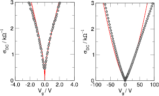
Figure 9. Comparison between the ab initio semiclassical conductivity (red lines) and the experimental data (circles) for suspended graphene (left panel, (Bolotin et al 2008)) and for graphene supported on SiO2 (right panel, (Novoselov et al 2005a)).
Download figure:
Standard image High-resolution image2.6.3. Quantum transport.
The semiclassical approach for the calculation of conductivity is not suitable to describe the conductivity near the Dirac point where quantum interference effects become important (Adam et al 2009). In this energy region both experiments and theoretical predictions claim that graphene is characterized by a non-vanishing conductivity, despite the vanishing density of states (Peres 2010, Das Sarma et al 2011, Katsnelson 2012). While calculations for ideal graphene predict a value  equal to
  the theoretical predictions for disordered graphene depends on the method adopted (Ziegler 1998, Katsnelson 2006, Tworzydło et al 2006, Ziegler 2006, Cserti 2007, Ziegler 2007) and the measured values are about two times larger (2e2/h) (Novoselov et al 2005a, Zhang et al 2005). This discrepancy stimulated an intense debate on the origin of the quasi-universal value of the conductivity minimum, ultimately leading to the conclusion that its value is related to the degree and nature of disorder in the carbon sheet (Suzuura and Ando 2002, Peres et al 2006, Schuessler et al 2009, Sajjad et al 2015). In particular, the minimal conductivity increases with disorder (Bardarson et al 2007, Titov 2007) and remains essentially constant when the temperature Ts is lowered by several orders of magnitude down to 30 mK (Tan et al 2007), where Anderson localization is expected (Das Sarma et al (2011) and reference therein). The absence of localization in graphene in the intermediate disorder regime indicates that the dominant disorder is either of long range character (Nomura and MacDonald 2007) and does not mix valley (Ostrovsky et al 2007) or preserves a chiral symmetry of the Hamiltonian (Ostrovsky et al 2010).
Hydrogen atoms, and resonant scatteres in general, have been envisioned as possible contributors to the minimum of conductivity (Stauber et al 2008) via the midgap states generated near the Dirac cones (Yuan et al 2010). These zero energy modes, that are proper of chiral symmetric graphene, are unaffected by Anderson localization and inelastic scattering effects, thereby giving rise to a robust metallic state characterized by a value of the conductivity independent of the impurity concentration (Ferreira and Mucciolo 2015), at least for ideal graphene with exact e–h symmetry.
The approach presented in the section 2.6.2, by addressing one (or a few) defects at a time, cannot describe localization effects, but intrinsically accounts for the quantum behavior of the electron dynamics in a complete ab initio way. Here, without attempting to justify the value of the minimum of conductivity that was the subject of several investigations (Peres et al 2006, Mucciolo and Lewenkopf 2010, Das Sarma et al 2011), we mention that our calculations do show a universal behavior at the Dirac point, i.e. one that depends on neither the dimensions of the model device used nor the nature of the impurity (being it a hydrogen or a fluorine atom, or a carbon atom vacancy). We shall address this issue in a future publication (Achilli and Martinazzo 2018).
2.7. Spin relaxation in spin transport
In addition to the resonant state and the related charge scattering phenomena, isolated hydrogen adatoms introduce also local magnetic moments that generate a spin-dependent behavior in the electron transport. Such spin transport, experimentally evidenced as a magnetoresistance effect associated to long range magnetic order, attracted considerable attention because observations find a rather long spin diffusion time. This quantity is intrinsically high in pristine graphene and may be considerably enhanced by hydrogen adsorption (Wojtaszek et al 2013). Nevertheless, different measurements also reported a reduced spin diffusion length (w.r.t. graphene), apparently due to 'magnetic' impurities such as hydrogen. These contradicting findings may arise from the different roles that the spin–orbit coupling and the spin exchange effects play in spin transport. Indeed, while the former (enhanced by hydrogen adsorption) reduces the spin diffusion time, the second lead to magnetic resonances that seems to act in the opposite way. Both Kochan et al (2014) and Soriano et al (2015) agree in identifying hydrogen adsorption as a mechanism improving the spin diffusion mechanism, but they disagree on the estimated hydrogen abundances necessary to fit exprimental data. Thomsen et al (2015) showed that a 5 ppm hydrogen defect density is sufficient to reduce the spin relaxation length to 2 μm, and that the inverse spin relaxation length and sheet resistance scale nearly linearly with the impurity concentration. Kamalakar et al (2015) measured a spin lifetime of the order of 1 ns, that agree well with theoretical predictions (Lundeberg et al 2013) identifying the impurity-induced magnetic spin flip mechanism as the factor prevailing on spin–orbit-coupling effects (Kochan et al 2014).
2.8. Paramagnetism
We have seen in the previous sections that a hydrogen atom adsorbed on graphene introduces a midgap state in its neighborhoods which, at charge neutrality, is singly occupied. Thus, in dilute systems—where hybridization does not occur—each defect-induced level may act as a spin-half paramagnetic center, i.e. a 'localized magnetic moment'. A spin-half paramagnetic response has indeed been measured by Nair et al (2012) using superconductive quantum-interference magnetometry experiments on carefully controlled fluorinated and irradiated graphene samples, and assigned to impurity-induced π moments. (The vacancy-related magnetic response has been shown to have a dual origin: one due to a σ moment, which is unaffected by charge doping, and one due to a π moment, which can be quenched upon shifting the Fermi level (Nair et al 2013). There remains to understand though why the two moments are not coupled to each other, despite the sizable exchange splitting between them (Casartelli et al 2013)). Though such measurements have not been undertaken for hydrogenated graphene, the detailed experimental and theoretical investigation by Gonzalez-Herrero et al (2016) of the local electronic structure around a H adatom gives a rather strong support that such behavior should be found for H atoms too (figure 7). Gonzalez-Herrero et al unambiguously assigned the double-peak structure observed in the differential conductance to a magnetic origin, i.e. to the Coulomb-splitted energy levels that host a localized magnetic moment.
It is worth noticing though that the localized magnetic moments associated with H adatoms in graphene differ substantially from those discussed by Anderson in his celebrated work (Anderson 1961). In the latter case, it is the impurity level that hosts the magnetic moment, and the associated resonance may lie considerably below the Fermi level (and be relatively broad) thanks to the strong Coloumb repulsion in the impurity level that prevents double occupation up to rather large values of the excitation energy. This situation does arise in H-graphene, but only when the adatom is pull out of the surface and the unpaired electron localizes into its 1s level. In the situation of major interest, instead, strong hybridization of the impurity level with the pZ orbital of the binding site creates a bonding energy level well below the Fermi energy and leaves a resonance state in the host material (section 2.5). The latter is rather sharp and lies close to the Fermi level, in such a way that even a relatively weak Coloumb repulsion prevents it to be doubly occupied. In other words, the zero energy modes extend over large regions, are built from the same π states responsible for conduction and no hopping exists with the latter.
The question arises whether the π moment can be quenched, at least partially, by interacting with conduction electrons—a common issue in metallic systems connected to the Kondo effect and, in turn, closely related to the Anderson problem (Schrieffer and Wolff 1966, Hewson 1993). In fact, charge transport measurements at low temperature on graphene-irradiated samples showed a logarithmic increase of the resistivity indicative of a spin-half Kondo effect (Chen et al 2011), but explanations involving electron-electron interactions in the disordered system are equally plausible (Jobst et al 2012, Chen et al 2012). The problem of how π midgap states interact with conduction electrons has been considered theoretically by Haase et al (2011), who combined dynamical mean-field theory with quantum Monte Carlo simulations to solve a model for a resonant scatterer including locally the electron-electron interactions, that is, with a Hubbard on-site repulsive term. The results of such calculations show that the magnetic susceptibility retains Curie-law behavior down to the lowest temperatures, thereby suggesting a ferromagnetic coupling between the π moment and the conduction electrons, in agreement with the observation of a paramagnetic response.
In concluding this section, we mention that the presence of a spin-1/2 moment also affects the formation of H2. This is because when using unpolarized H atom beams only 1/4 of the atom pairs has the correct (singlet) symmetry for the reaction to occur. In the triplet state the interaction between the projectile H atom from the gas-phase and the target H atom chemisorbed on the surface is largely repulsive, and the reaction prevented. This leads to the introduction of a 1/4 spin-statistical factor to weight properly the dynamical results based on a single electronic state (section 2.4).
3. High coverage
In this section we address the consequences that the adsorption of the first few hydrogen atoms has on the properties of the graphene sheet, starting from those (chemical) that make the adsorption process itself not trivial.
3.1. Preferential sticking and dimer formation
The presence of singly occupied energy states that localize on specific lattice positions has of course some consequences for the chemical reactivity of defective graphene substrate. This occurs because, as discussed in section 2.1, chemisorption of hydrogen atoms (and likely of many other species that covalently bound to the substrate) is an activated process, and thus any change in the height of the energy barrier to sticking reflects exponentially on the kinetics of the adsorption process. This leads to formation of dimers and clusters on the surface that make the adsorption kinetics non-trivial. Were not for such a barrier the sticking of atomic hydrogen would remain random, and only in conditions of full thermodynamic equilibrium15, rarely realized in a surface science experiment, dimers and clusters would emerge as abundant species (because of their thermodynamic stability).
Dimer formation and clustering were unambiguously shown to occur when imaging with STM the structures that hydrogen atoms form when dosed from a hot (1600–2200 K) beam source (Hornekær et al 2006a, Balog et al 2009) (see figure 10). The monomers observed at low coverages—with their relatively short room-temperature lifetime of some minutes—were replaced by more stable structures when increasing the exposure, already at a coverage of ∼0.2%. This occurred in spite of the fact that H monomers are immobile on the surface (section 2.3), a rather unusual situation for aggregation of adspecies on a surface. Hornekær et al (2006a), supported by DFT calculations, showed that this could only be due to a 'preferential sticking' mechanism that favors adsorption of a second atom in specific lattice positions around a first adsorbed species. This is clearly related to the defect-induced midgap states (section 2.5) that are introduced in the substrate at earlier times of the exposure and that influence subsequent chemical reactivity of the substrate.
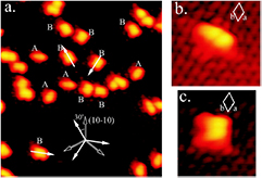
Figure 10. Hydrogen dimer structures on graphite at a coverage of ∼1%. (a) STM image (103 × 114  ) of ortho (A) and para (B) dimers. Black arrows indicate the
  directions and white arrows indicate the orientation of the dimers 30° off. (b) Close up of the ortho dimer structure. (c) Close up of the para dimer structure. Reproduced from Hornekær et al (2006b), Copyright 2006 by the American Physical Society. See also Balog et al (2009) for details on the same structures on epitaxial graphene on SiC(0 0 0 1).
Download figure:
Standard image High-resolution image3.1.1. Site-magnetization and barrier to sticking.
The rationale for the preferential sticking mechanism is best given in terms of the RVB model introduced in section 2.5 (Casolo et al 2009a). Assuming that a first H atom adsorbs on an A-type site, the unpaired electron left on the B sublattice may easily (i.e. with a small or even vanishing activation barrier) couple to the electron of an incoming H to form a CH bond. Hence, formation of a 'AB dimer' is an easy process, and a singlet ground-state results in which the aromaticity of the substrate is partially restored. Conversely, if secondary adsorbtion occurred on the same sublattice to form an 'A2 dimer', the incoming H atom would not take advantage of the available unpaired electron density (spin density), and adsorption would be as difficult as the first one. This is shown in figure 11 that reports the results of DFT calculations on a number of dimers as a function of the site-integrated magnetization, which is a measure of the average number of unpaired electrons available and roughly equals  for the midgap state wavefunction at that site. Binding (barrier) energies are seen to increase (decrease) linearly by increasing the local magnetization, thereby showing how the spatial distribution of the midgap state determines the thermodynamic stability and the chemical reactivity. The result is a genuine electronic effect (in principle tunable by charge doping (Huang et al 2011)): substrate relaxation effects, though substantial, are site-independent for all but the so-called ortho dimer (with two Hs on neighboring sites), since surface puckering upon adsorption involves to a first approximation nearest-neighboring C atoms only. Recently, a detailed look at the relaxation effects has been provided by Zhang et al (2018) who used DFT calculations on large supercells to investigate the A–A and A–B interactions at long range. It has been found that the deformation potential makes the H–H interactions always attractive, though the A–B ones turn out to be much larger than the A–A one.
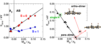
Figure 11. Left panel: binding energies for secondary H adsorption (with a first H atom in A lattice position) as a function of the site-integrated spin-density (MSI). Results are shown for AB ( ) and A2 (
 ) dimers, in both their singlet (red) and triplet (blue) states. Right panel: corresponding barrier energies for secondary atom adsorption (ground-state only). Data point at
  is for single H adsorption as indicated. The insets show the geometry of the para- and ortho- dimers, as indicated. Reprinted with permission from Casolo et al (2009a). Copyright 2009, AIP Publishing LLC.
Download figure:
Standard image High-resolution image3.1.2. Reaction versus dimer formation.
The formation of dimers raises the issue of the competition between the ER reaction and secondary adsorption. Modeling the dynamics is quite challenging because it requires the development of a fully corrugated potential model that accounts for H2 formation as well as for sticking at, at least, the ortho and para positions. The problem was solved by Casolo et al (2013) and (2016) in a classical though ab initio setting, i.e. with the help of AIMD. The advantage of the technique is that it avoids the need of computing and fitting a complicated potential, energies and forces being computed as required by the dynamics itself. The results of Casolo et al (2013) and (2016) showed the expected preferential formation of 'balanced' dimers, with the para dimers being the most abundant ones (up to one-half the total dimer fraction). Formation of these dimers features a dynamical threshold of ∼20 meV (corresponding to a beam temperature  K), below which only recombination is possible. This agrees well with the findings of Areou et al, who observed complete refreshment of a pre-covered surface upon exposing it to a low energy H atom beam (Aréou et al 2011).
Overall, ER abstraction dominates over dimer formation for collision energies smaller than ∼0.2 eV. Nevertheless, accounting for the effects that formation of dimers may have in H2 recombination was found to be crucial to improve the agreement between theory and experiments on the size of the reaction cross-section (Zecho et al 2002b). The cross-section obtained by Casolo et al of 3.1 ± 0.2  at ∼0.20 eV (corrected for the spin-statistical factor) agreed well with the value of ∼3.5
  measured by Zecho et al at saturation for the same energy (that is, subtracting off the HA contributions, see section 2.4).
3.2. High temperature dimer recombination
Early observations of thermally activated molecular hydrogen formation were puzzling because of a double peak structure in the thermal desorption spectra, with a main peak for H2 (D2) at 445 K (490 K) and a minor peak at 560 K (590 K), as well as a first order desorption kinetics (Zecho et al 2002a). These findings was clearly incompatible with a monomer desorption barrier of ∼1 eV (the sum of the adsorption energy  eV and the adsorption barrier of 0.2 eV) that is expected to give a single thermal desorption spectroscopy (TDS) peak around
  K. It took some time before formation of dimers was fully appreciated and thermal desorption spectra correctly interpreted as activated formation of molecular hydrogen from ortho and para dimers on the surface (Hornekær et al 2006b). In a combined experimental and theoretical effort, Hornekær et al (2006b) were able to show that, despite their similar binding energies, ortho dimers are more stable against thermal annealing, and at surface temperatures of ∼500 K (between the two TDS desorption peaks) they are the only species present on the surface. As a result, para dimers contribute to the first desorption peak while ortho dimers contribute to the second one.
DFT calculations found a barrier for H2 formation out of the para dimer of ∼1.4 eV, in agreement with the temperature of the first peak in the TDS spectra. Conversely, direct recombination out of the ortho dimer was found to have a large barrier of 2.5 eV, preventing direct recombination out of this structure (see insets of figure 11). Instead, at the temperature of the second peak in the TDS spectra, ortho dimers convert into para dimers and recombine. Since the rate limiting step for this reaction (the 'diffusion' of a H atom in para position) has a barrier of ∼1.6 eV, this determines the second TDS peak (Hornekær et al 2006b). DFT calculations also showed that recombination from larger cluster structures generally occur at para dimer-like edges with barriers similar to that of the para dimer (Šljivančanin et al 2011).
3.3. Lattice softening and clustering
Increasing hydrogen atom exposure, aggregates of increasing number of atoms appear on the surface. For them the preferential sticking as described above does not apply, since after forming an AB dimer no further unpaired electron is available to bias the adsorption of additional H atoms in specific lattice positions. This is confirmed by DFT calculations, which show that adsorption of a third hydrogen atom to a stable AB dimer is quantitatively similar to the first H adsorption event (Casolo et al 2009a). Energy barriers for further adsorption follow a similar trend: barriers for sticking a third H atom compare rather well with that for single H atom adsorption for the processes AB → A2B and A A3, and are considerably smaller for A
 A2B ones. Nevertheless there exist exceptions when forming compact clusters. The reason for them appears twofold. On the one hand, some structures are more favored than others because the relaxation energy is lowered around sites that have already sp3 character, a kind of substrate softening that occurs upon adsorption. On the other hand, a dimer or a cluster on the surface introduces 'edges' in the π cloud, and these are known to be more reactive than 'bulk' lattice sites (see section 4), hence favor cluster growth.
Overall, the combined effect of substrate and electronic effects provides the necessary driving force for clustering of adatoms. When the cluster is unbalanced (i.e. with different numbers of adatoms in the two sublattices) there exist strong electronic effects for adsorbing a H atom close to the cluster since, similarly to the formation of dimers described above, there exist unpaired electrons (midgap states) available, see the next section. When the cluster is balanced, on the other hand, lattice softening and (weaker) electronic effects provide good reasons for cluster growth.
3.4. Predicting midgap states
The appearance of midgap states is a common feature of bipartite systems, which has long been investigated in aromatic systems and rediscovered several times in different contexts. Here, for the sake of precision, we say that a system is bipartite system when its Hamiltonian takes an off-block diagonal form,  , where A, B identifies two complementary subspaces of the Hilbert state space and (call PA and PB the corresponding projectors)
  , etc. This is clearly the case of graphene with only nearest-neighboring hoppings, where A and B identify with the spaces spanned by the pZ orbitals of the two sublattices, provided the zero of energy is set to that of the isolated pZ orbitals. A simple result can then be stated as follows (Inui et al 1994, Yazyev 2010): in any bipartite lattice in which the numbers of sites in the two sublattices (NA and NB, respectively) differ, there exist at least
  linearly independent eigenfunctions of the Hamiltonian at zero energy, all with null amplitudes on the minority sublattice sites. The proof is simple: for let
  and
and ![$ \renewcommand{\ket}[1]{|#1\rangle} \ket{\psi}=\sum_i b_i\ket{\beta_i}$](https://content.cld.iop.org/journals/0953-8984/30/28/283002/revision2/cmaac89fieqn177.gif) be a trial solution at zero energy, with
be a trial solution at zero energy, with ![$ \renewcommand{\ket}[1]{|#1\rangle} {\ket{\beta_i}}$](https://content.cld.iop.org/journals/0953-8984/30/28/283002/revision2/cmaac89fieqn178.gif) a complete set in B; the coefficients bi need to satisfy
a complete set in B; the coefficients bi need to satisfy ![$ \renewcommand{\bra}[1]{\langle#1|} \renewcommand{\braket}[1]{\langle#1\rangle} \sum_i \braket{\alpha_j|H|\beta_i}b_i=0$](https://content.cld.iop.org/journals/0953-8984/30/28/283002/revision2/cmaac89fieqn179.gif) for j = 1,2,..NA, which is a set of NA equations for the
for j = 1,2,..NA, which is a set of NA equations for the  coefficients bi, that is, having at least η linearly independent solutions. This also shows that the zero-energy modes localize on the majority (B lattice) sites.
The above arguments prove the so-called imbalance rule, a very useful result in graphenic systems, which gives the minimum number of zero energy modes to be expected. More generally, it is the concept of nonadjacent sites in an N-site bipartite system that largely determines the number of such states (Longuet-Higgins 1950, Fajtlowicz et al 2005, Yazyev 2010). We say that two sites are nonadjacent if they are not bound (connected by a transfer integral) to each other; for instance, two sites on the same sublattice are nonadjacent. Clearly, there exists a maximal set of nonadjacent sites and we call β the sites in this set, and α the remaining ones ( in number, respectively). Each site β binds at least one site α, otherwise it would be completely isolated and could be removed at the outset. Arranging one electron per site, however, we can form at most
  bonds at a time, and therefore we are left with
  unpaired electrons. Equivalently, we end up with
  midgap states that necessarily localize on the maximal set of nonadjacent sites. Eventually, we can restate this result by defining η to be the number of unpaired electrons in the Lewis structure(s) with the maximum number of bonds, i.e. for π bonds in graphenic systems, the principal resonance structures.
Rigorously speaking (Fajtlowicz et al 2005), for a generic (bipartite) system this result gives yet a lower bound only to the number of zero energy states,  , although greater or equal than the above one based on the lattice imbalance (the reader may easily recognize that the latter is just a special result of this counting rule). In fact, there may exist further states at zero energy for specific values of the hoppings (H matrix elements), which are known as supernumerary modes (Longuet-Higgins 1950). However, they cannot occur in hexagonal (benzenoid) systems for which
  strictly holds.
All these results become largely relevant to 'real' graphene because e–h symmetry (bipartitism) holds to a large extent. A huge number of numerical calculations exist, both at the tight binding and at DFT level of theory, confirming the appearance of zero-energy modes associated with pZ vacancies.
3.5. Magnetic ordering
Having discussed in section 2.8 some of the magnetic properties of diluted H atom species adsorbed on the surface, we can now focus on the possibility that interactions between moments lead to ferromagnetic order, a long-standing issue for the search of s − p magnetism. Ferromagnetism in graphite and later in graphene has been reported (Esquinazi et al 2002, 2003, Barzola-Quiquia et al 2007, Wang et al 2009) but later questioned in the light of the ubiquitous presence of magnetic contaminants. Subsequent measurements under carefully controlled conditions have indeed shown that graphene, like graphite, is strongly diamagnetic and has only the weak paramagnetic contribution described above due to adatoms and/or carbon atom vacancies (Sepioni et al 2010).
Coupling between defects may in principle give rise to magnetically ordered structures if it favored the parallel alignment of π moments of the defect-induced midgap states. Such situations are entirely determined by electron correlation, and require that Coulomb repulsion is correctly taken into account. If this is done at the level of on-site repulsion—that is, in the framework of the repulsive Hubbard model (Hubbard 1963)—a theorem due to Lieb gives a definite answer to this question (Lieb 1989): he proved that for any bipartite system at half-filling the ground-state spin S is determined by the sublattice imbalance only, namely as  . No matter how many midgap states are present (remember that
  ) it is the sublattice imbalance that governs spin alignment16. In the simplest situation where
  coupling between π moments is ferromagnetic when adatoms (or C atom vacancies) are placed on the same sublattice and antiferromagnetic otherwise. This is a rather sound result that can be understood by considering 'interactions' between midgap states: hybridization occurs when impurities sit on different sublattices (non-zero hopping matrix elements involve different sublattices), and favors antiferromagnetic coupling in place of an otherwise dominant parallel-spin alignment. Similar results follow by analyzing the RKKY interactions between local magnetic moments
  placed at different lattice positions, i.e.
  where J is the contact exchange between the host electrons and the magnetic impurity and
  is the real-space spin susceptibiliy. It is indeed found that the coupling is ferromagnetic for moments in the same sublattice (
 ) and antiferromagnetic otherwise (
 ), and that it has a characteristic R−3 dependence on the distance in place of R−2 found for ordinary 2D metals (Kogan 2011, Sherafati and Satpathy 2011a, 2011b).
Lieb's result sets important constraints for building up macroscopic magnetic moments: ordered domains can only be obtained if defects are unevenly distributed between the two sublattices. Though this is hardly achievable in ordinary situations, manipulation of H atoms adsorbed on graphene has been shown possible with STM, and full control over sublattice population achieved (Gonzalez-Herrero et al 2016). A transient sublattice imbalance (and ensuing ferromagnetism) has been suggested for bilayer graphene and graphite (Moaied et al 2014, 2015). This would arise because of the (small) sublattice dependence of the hydrogen binding energy that originates from layer stacking: desorption is faster for weaker bound species, hence a temporary sublattice imbalance appears when desorbing H atoms from the surface (Moaied et al 2015). Though reasonable and appealing, the argument relies on the existence of a random configuration of monomers on the surface at initial times, a condition that—as seen above—is realized only at very small coverages, likely irrelevant for practical purposes (Bonfanti and Martinazzo 2018).
3.6. Metal–insulator transition and electron localization
The spin ordering illustrated in the previous section determines also a peculiar behavior of the transport properties of H-functionalized graphene in high disorder limit. It was indeed demonstrated that if the impurity distribution gives rise to ferromagnetic ordering a ballistic conduction regime is maintained through a robust metallic state. Differently, when non magnetic ordering is established by random adsorption of impurities, hydrogenated graphene display insulating properties. Such metal–insulator transition is related to Anderson localization induced and maximized by the large disturbances introduced by hydrogen impurities. In particular point defects introduce a new length parameter which can be related to the decay length of the midgap state. The quantum interference effects leading to Anderson localization become relevant when the distance between impurity decreases up to this length. In such conditions the spectrum undergoes a rearrangement with the opening of a quasi-gap around the impurity resonance (Skrypnyk and Loktev 2011). Hydrogenated graphene has also been used recently as model to explain metal–insulator transition in two dimensions (Osofosky et al 2016).
3.7. Graphane
It is clear from the previous arguments that an amorphous product is likely to form, with little (if any) crystalline order, when graphene is exposed to large doses of hydrogen atoms. Annealing helps in relaxing strain, but forming crystalline hydrogenated form of graphene in this way appears unlikely.
Graphane is the best-known form of ordered hydrogenated graphene, the fully hydrogenated form with a H atom per each carbon atom, alternating above and below the surface plane (Sofo et al 2007). Graphane is structurally robust and has been predicted to exhibit a rather high thermal stability that makes possible its use in two-dimensional electronics (Openov and Podlivaev 2010). However, for the same reasons, it can hardly be considered as a promising hydrogen storage material, unless it is properly functionalized (Zhou et al 2014, Shiraz and Tavakoli 2017). Its formation requires a perfect correlation between the sublattice position and the surface face, something which is somewhat at odds with the above discussed tendency to form 'balanced' structures. Indeed, such tendency holds irrespective of the surface face and, at any step of the hydrogenation process, it hardly 'distinguishes' the top from the bottom surface, when they are both made available to the hydrogen flux. For dimers, for instance, the so-called syn- and anti-configurations (respectively, with the two atoms on the same or on the opposite faces) are energetically so close in energy that they can be considered equally likely for any practical purposes.
The formation of crystalline graphane is indeed yet to be realized (Pumera and Wong 2013). Evidences for graphane-like domains in a reversible hydrogenation process (Elias et al 2009) are often quoted incorrectly as 'graphane synthesis', despite the lack of sufficient support for the realization of crystalline CH. In their experiments, Elias et al (2009) exposed either free standing or Si/SiO2 supported graphene to a hydrogen plasma till saturation, and used Raman spectroscopy, TEM and electric measurements to characterize their samples. From Raman intensities they found that the degree of hydrogenation of graphene membranes was twice as large as for supported graphene ( ratios of about 2:1 and 1:1 respectively). This suggests that graphene on a Si/SiO2 is only one-sided hydrogenated, hence with a saturation coverage ⩽40%; in fact, it is also non-crystalline, as evidenced from the transport characteristics (Elias et al 2009). Free-standing graphene, on the other hand, showed some degree of crystallinity but contained only twice the number of H atoms of supported graphene. And an
  ratio of 2:1 is believed to be yet too small for a 1:1 stoichiometry, namely it presumably corresponds to a coverage <10% (Pumera and Wong 2013) (larger values of such ratio can be found in the literature (Smith et al 2015), despite no superhydrogenated form of graphene is known to exist). Thus, a different, presumably ordered hydrogenated graphene is likely to be formed but with some different stoichiometry CnH (n > 1). To date, the highest degree of graphene functionalization, approaching 1:1 stoichiometry, has been achieved by fluorination (Robinson et al 2010).
4. Adsorption at edges and point defects
4.1. Edge reactivity
Edge functionalization (Bellunato et al 2016) is known to largely affect the properties of graphene structures, and a variety of elements are known to attach to the edge of graphene. Hydrogen is the most elusive to study due to its small atomic mass, though it easily saturates the termination because this lowers the edge energy. In fact, saturation of the σ dangling bonds with hydrogen atoms is a facile process, with a binding energy per atom that may well exceed 5 eV and typically fall in the range 4–5 eV for an irregularly shaped edge (Migliorini 2014). Lower values are found at armchair-shaped segments since they are stabilized by a C–C bond contraction (to ∼1.25 Å) and formation of quasi triple bonds (in alkynes the C–C bond length is ∼1.20 Å), as shown theoretically (Kawai et al 2000) and observed experimentally (He et al 2014). Hydrogen-free zig-zag edges are known to reconstruct too, and to attain a pentagonal-heptagonal rearranged structure that is even more stable than the reconstructed armchair one (Koskinen et al 2008). In turn, this makes dissociation of H2 endothermic, hence it should 'self-passivate' the edge with respect to hydrogen adsorption from a molecular atmosphere. However, lonely zig-zag segments may be found in irregularly shaped edges with little chance to reconstruct, and H adsorption at these sites is yet largely favored ( eV, close to the value of 5.3 eV appropriate for the unreconstructed edge). The structure and thermodynamic stability of bare and hydrogenated nanoribbon-edges in H2 atmosphere were investigated with DFT by Wassmann et al (2008), and rationalized with the help of simple chemical concepts relying on Clar's formulas. In the following, we focus on the π reactivity only (i.e. we imagine to start from hydrogen terminated edges) and introduce simple arguments, that apply equally well to both regularly and irregularly shaped edges, to predict the site-dependent tendency to (further) hydrogenation.
4.1.1. Lattice renormalization and hyperconjugation.
Low energy orbitals show a marked tendency to localize at the edge sites, irrespective of whether or not they are regularly shaped. This is a consequence of e–h symmetry, i.e. of the symmetry of the tight-binding Hamiltonian with nearest-neighbors interactions only,  (see section 3.4). To show this, we perform a lattice 'renormalization' (Naumis 2007, Martinazzo et al 2010) and focus on one sublattice only (say
  ) and on the 'renormalized' Hamiltonian
  . Indeed, since H only allows transitions from the A to the B subspaces (HBA) and vice versa (HAB) it is sufficient to consider the problem in the A space only with the Hamiltonian17
  .
.
The spectral properties of  are closely related to those of the original Hamiltonian H. For any non-zero eigenvalue
  and eigenvector
 ![$ \renewcommand{\ket}[1]{|#1\rangle} \ket{\psi_{A, i}}$](https://content.cld.iop.org/journals/0953-8984/30/28/283002/revision2/cmaac89fieqn204.gif) of this Hamiltonian there exist two solutions of the original problem with eigenvalues
of this Hamiltonian there exist two solutions of the original problem with eigenvalues  and eigenvectors
 ![$ \renewcommand{\ket}[1]{|#1\rangle} \ket{\psi_{A, i}}\pm\ket{\psi_{B, i}}$](https://content.cld.iop.org/journals/0953-8984/30/28/283002/revision2/cmaac89fieqn206.gif) , where
, where ![$ \renewcommand{\ket}[1]{|#1\rangle} \ket{\psi_{B, i}}$](https://content.cld.iop.org/journals/0953-8984/30/28/283002/revision2/cmaac89fieqn207.gif) is defined to be
is defined to be ![$ \renewcommand{\ket}[1]{|#1\rangle} \newcommand{\e}{{\rm e}} \ket{\psi_{B, i}}=\tilde{\epsilon}_{i}^{-1/2}H_{BA}\ket{\psi_{A, i}}$](https://content.cld.iop.org/journals/0953-8984/30/28/283002/revision2/cmaac89fieqn208.gif) (if
(if  ,
, ![$ \renewcommand{\ket}[1]{|#1\rangle} \ket{\psi_{A, i}}$](https://content.cld.iop.org/journals/0953-8984/30/28/283002/revision2/cmaac89fieqn210.gif) is already a H eigenvector). The converse is also true, namely from any eigenvector
is already a H eigenvector). The converse is also true, namely from any eigenvector ![$ \renewcommand{\ket}[1]{|#1\rangle} \ket{\psi_{i}}$](https://content.cld.iop.org/journals/0953-8984/30/28/283002/revision2/cmaac89fieqn211.gif) the two projections
the two projections ![$ \renewcommand{\ket}[1]{|#1\rangle} \ket{\psi_{A, i}}$](https://content.cld.iop.org/journals/0953-8984/30/28/283002/revision2/cmaac89fieqn212.gif) and
and ![$ \renewcommand{\ket}[1]{|#1\rangle} \ket{\psi_{B, i}}$](https://content.cld.iop.org/journals/0953-8984/30/28/283002/revision2/cmaac89fieqn213.gif) onto the A and B subspaces satisfy
onto the A and B subspaces satisfy ![$ \renewcommand{\ket}[1]{|#1\rangle} \newcommand{\e}{{\rm e}} H_{BA}\ket{\psi_{A, i}}=\epsilon_{i}\ket{\psi_{B, i}}$](https://content.cld.iop.org/journals/0953-8984/30/28/283002/revision2/cmaac89fieqn214.gif) and
and ![$ \renewcommand{\ket}[1]{|#1\rangle} \newcommand{\e}{{\rm e}} \tilde{H}_{AA}\ket{\psi_{A, i}}=\epsilon_{i}^{2}\ket{\psi_{A, i}}$](https://content.cld.iop.org/journals/0953-8984/30/28/283002/revision2/cmaac89fieqn215.gif) ; that is, in studying
; that is, in studying  one only misses possible zero eigenstates in the B subspace, that can be easily detected by defining A to be the majority species and comparing the number of zero A eigenstates with the sublattices imbalance. Importantly, the above lattice renormalization maps the low-energy side of the excitation spectrum of the original problem into the low-energy sector of
  : the ground-state of the renormalized system corresponds to the highest occupied/lowest unoccupied molecular orbital (HOMO/LUMO) pair of the original system—the so called frontier orbitals. Frontier orbitals are key quantities because, from a chemical perspective, they govern the system chemical reactivity to a large extent (Fukui et al 1954), similarly to what midgap states do when unpaired electrons are present. Hence, the ground-state of the renormalized problem is a powerful tool to investigate the reactivity, a quite unique situation.
The renormalized lattice of a honeycomb lattice (see section 2.5.2, with NN hoppings only) is a hexagonal (commonly referred to as 'triangular') lattice, that is of course the sublattice  of the original system, with different parameters. The renormalized hopping is just t2 (assuming tij = t for simplicity), while the on-site energies are
  , where Zi is the coordination number of the ith A site in the original lattice, a sort of 'π-coordination number'. In the bulk of graphene Z = 3 but at an edge such number is smaller, typically Z = 2, though Z = 1 is also possible18. Of course, the ground-state of the renormalized lattice tends to localize on the sites with the lowest on-site energy; hence, frontier orbitals of the original π system must show a certain degree of edge localization. Furthermore, among the edge sites, the ground-state of the fictitious problem localizes mainly on the sites with the largest number of similar neighbors in the renormalized lattice—next-to-nearest neighbors in the original lattice—since this situation maximizes the degree of hybridization. Hence the number (ξ) of next-nearest-neighbors provides further insights into the nature of the edge state (Bonfanti et al 2011b). We named it the hypercoodination number since, unfortunately, the more appropriate term hyperconjugation was already in use in the chemical literature, with a rather different meaning. Its usefulness becomes soon evident when considering the textbook cases of armchair and zig-zag edges. The 'true' edge sites are two-fold π coordinated in both cases (Z = 2) but the hypercoordination is larger for the zig-zag (
 ) than for the armchair (
 ) one, and this suggests a more marked edge localization (and reactivity) for the first.
4.1.2. Adsorption energetics.
The combination of edge localization and sublattice imbalance (with its own sublattice localization) provides a set of useful rules that helps predicting graphene reactivity. Two different situations can be envisaged that alternate to each other in a sequential adsorption process at the edges (Bonfanti et al 2011b, Jensen et al 2018).
In the absence of unpaired electrons reactivity is largest at the edge sites with lowest Z and largest ξ. The prototypical cases is H atom adsorption at a perfect (H-terminated) zig-zag edge, where the binding energies is  eV, i.e. much larger than for a 'bulk' site (
 eV, see section 2.1). DFT (and higher theory level) calculations on a number of graphene clusters of different size and shape showed that the H binding energy at the Z = 2 sites of irregularly shaped edges fall all between the above mentioned limits, with a clear preference for sites with largest ξ (Bonfanti et al 2011b). Because of its nature the ξ number may fail when comparing sites in different systems, but it is rather robust when used within the same structure. In addition, reliable upper bounds for the binding energy exist: the one given above for perfect zig-zag edges is the largest (useful for
  ), smaller upper bounds are ∼1.7 eV for
  (the binding energy for the perfect armchair edge) and ∼1.3 eV for
  . For 'bulk'-like graphenic sites (Z = 3), on the other hand, ∼1.0 eV can be considered a reliable bound.
When the adsorbed hydrogen atoms leave a sublattice imbalance on the surface, one or more unpaired electrons (midgap states) appear. Similarly to those discussed in section 5, such states localize on the majority sublattice but they are now shaped by the presence of the edge, showing a preference for small Z and large ξ sites, for the same reasons given above. Binding hydrogen atoms on such sites is rather easy and binding energies can be rather large, up to ∼3.0 eV for Z = 2, ∼3.8 eV for Z = 1 and ∼4.0 eV for Z = 0 (the binding energy for forming the para dimer provides the right figure for the case Z = 3,  eV).
eV).
As a consequence, hydrogen atoms—when employed under mild reaction conditions that prevent bulk adsorption—should start binding at the edges and 'corrupt' the graphene sheet by reducing the spatial extension of its π cloud. In this way, as hydrogenation proceeds carbon atoms that were initially in the bulk (hence relatively inert) can find themselves at the 'moving' edges of the π cloud (Z = 2) or be even isolated from it ( ), thereby becoming rather prone to hydrogenation. That reaction can indeed proceed starting from the edges has been shown with Birch-type 'wet' hydrogenation (Zhang et al 2016) on mechanically exfoliated graphene (figure 12). Birch reduction is a hydrogenation reaction that has been long used to partially hydrogenate aromatic rings, e.g to convert aromatic rings into 1,4-cyclohexadienes. It differs from atomic hydrogen exposure19 but it involves yet the spatial properties of the frontier orbitals discussed above, since they are required to accommodate an electron from the reaction medium. Interestingly, only bilayer and few-layer graphene have shown edge-hydrogenation, the more reactive single layer graphene was seen to undergo uniform reaction.

Figure 12. Structural evolution of bilayer graphene during a Birch-type hydrogenation reaction, showing the evolution of the Raman AD/AG map (peak area ratios), (a) before, (b) after 2 min and (c) after 8 min reaction. Reprinted (adapted) with permission from Zhang et al (2016). Copyright 2016 American Chemical Society.
Download figure:
Standard image High-resolution image4.2. Carbon atom vacancies
Carbon atom vacancies may be important absorbers for hydrogen, since they get stabilized by hydrogen termination. They are typically introduced by electron or ion irradiation, although they may also form during the fabrication process. Controlled vacancy formation can be achieved using low energy electrons (∼100 keV) in the same transmission electron microscope used for their imaging (Meyer et al 2008, Krasheninnikov and Nieminen 2011). As created, the C atom vacancy presents one π midgap state due the removal of a pZ orbital and three σ dangling arising from the breaking of the σ backbone. However, a Jahn–Teller distortion occurs that determines a (five-membered) ring closure, thereby leaving only one dangling bond on a 'apical' C atom (El-Barbary et al 2003, Lehtinen et al 2004, Yazyev and Helm 2007, Dharma-wardana and Zgierski 2008, Palacios and Ynduráin 2012, Casartelli et al 2013). Bare vacancies are mobile on the surface and interact with each other (coalasce) to form divacant species that, being much more stable (by about 6.7 eV) than two separated single vacancies, dominate at equilibrium. In fact, the barriers to diffusion are relatively small (El-Barbary et al 2003) (1.4–1.7 eV) that the recombination kinetics is moderately fast already at operating temperatures for realistic concentrations of defects (Casartelli et al 2014).
The situation changes drastically in hydrogen atmosphere, since hydrogen atoms are expected to saturate all the three original σ bonds and lock the vacancy in place. DFT calculations showed that this is indeed the case (Casartelli et al 2014), and proved that in a wide temperature—H2 partial pressure range (comprising standard atmospheric conditions, i.e.  K and
K and  bar in dry atmosphere) the triply hydrogenated vacancy is the most abundant species on the surface up to
  K. The bare vacancy is thermodynamically stable only at high temperature and low hydrogen pressure, and thermal annealing at T > 1200 K (>800 K) would be required in atmospheric (UHV) conditions to free vacancy defects from hydrogen atoms (this has to be compared to
  K for desorbing H atoms and dimers from the basal plane). The triply hydrogenated structure has a residual π moment and, from the electronic structure perspective, is the analogue of the H monomer case discussed in section 2 (actually, the ideal case of a true pZ vacancy). Addition of a further hydrogen atom to the vacancy is energetically favored over the bulk, with
  eV that compares rather well to the binding energy to form the hydrogen ortho-dimer.
4.3. Boron- and nitrogen- doped graphene
There exist few species that can be inserted into the graphene lattice without drastically altering its geometric and electronic structure. Among these, boron and nitrogen are likely the best because their size introduces little strain into the structure keeping its planarity (though N is superior than B since its covalent radius of 71 pm compares much better than B (84 pm) with that of C (73 pm)). Both species act as charge dopant without altering the electronic structure, hence they are expected to increase the reactivity of the graphene sheet with respect to hydrogen (Huang et al 2011). Furthermore, depending on their concentration, they may partially or totally quench the magnetic moments that arise upon hydrogen adsorption, and transform the accompanying 'spin alternation' pattern into a 'charge alternation' pattern. Differently from physical doping (i.e. electrostatic gating), though, boron and nitrogen species also introduce charged centers that act as Coulomb scatterers for the conduction electrons and modulate the charge density. Hence, there is some basic interest in investigating hydrogen adsorption in the presence of chemical doping species. This is not only academic: B-doped graphane has been predicted to be a (conventional) high-Tc superconductor (Savini et al 2010), in analogy with the B-doped diamond realized experimentally (Ekimov et al 2004) ( K) but with a high superconducting temperature, ∼90 K.
These issues have been investigated with DFT calculations by Pizzochero et al (2015). These authors showed that hydrogen atom adsorption on carbon sites close to the dopant is favored (over pristine graphene) in both B- and N-doped graphene, and that the effect of the dopant is stronger at its ortho position. The binding energy at such position attains quite large values,  –2.1 eV, i.e. comparable to the adsorption of a second atom at an ortho or para position in pristine graphene. As expected, the doped system is and remains non-magnetic—at least till the ratio H:X (X = B,N) is less or equal to one—and the charge density around the dopant-impurity atom location shows a spatial behavior similar to that of the previously discussed midgap state. Adsorption on top of the dopant is (much) easier than on a carbon atom when the dopant is boron (
 eV), while it is more difficult when it is nitrogen (
 eV). This is mainly a structural effect as, upon adsorption, B bulges out the surface much less than N.
When considering dimers, it is seen that charge doping plays a major role and changes the relative stability of the doubly hydrogenated configurations. This is particularly the case of some meta structures—namely, those with both H atoms next to the dopant—that become very stable. In general, and similarly to undoped graphene, magnetic configurations always result when two H adsorb on the same sublattice. Contrary to graphene, however, a magnetization of only 1  per pair is observed in doped graphene, as a consequence of charge doping that partially quenches the magnetic moment.
5. Additional topics
5.1. Graphene versus other 2D materials
The discovery of graphene triggered a wealth of fundamental and applied studies on other atomic-thick 2D materials. The search of new 2D materials started from those which could be peeled off from natural crystals (e.g. BN, MoS2, MoSe2, WS2, WSe2, NbSe2, NiTe2, Bi2Se3, Be2Te3 and black phosphorus) through either mechanical (Novoselov et al 2005b) or chemical exfoliation (Coleman et al 2011), and rapidly evolved into the synthesis of novel layered materials.
5.1.1. Silicene.
Compelling evidence for silicene, the two-dimensional allotrope of Si, was first reported in 2012 (Vogt et al 2012). This material has attracted much attention from the community since the beginning, mainly because of the expectations of being easily integrated into the existing Si-based technology, partly met with the realization of the first silicene field effect transistors (Tao et al 2015). Silicene has a band structure very similar to graphene, with two Dirac cones at the corners of its hexagonal Brilluoin zone, and a very similar Fermi velocity. At a closer look, however, there exist marked differences. Silicene is not flat, rather presents a buckled structure that makes the sublattices distinguishable by e.g. application of an electric field. Hence, the Si atoms have some sp3 character on their own. It has further (much) weaker π (and σ) bonds, that implies that its lattice is softer than graphene. Thus, it is instructive to consider the hydrogenation process of silicene, and compare it with the situation in graphene (Pizzochero et al 2016).
Hydrogen adsorbs on silicene much like it does on graphene: the hydrogen atom binds on top a Si atom and triggers a (further) outward motion of the lattice atom. The energetics, though, are completely different: the binding energy is  eV, more than 1 eV larger than in graphene. This is the combined effect of structural and electronic factors. Since the lattice is softer, the reconstruction energy (the energy going into the substrate to create a binding Si with a full sp3 character) is only ∼0.1 eV, one order of magnitude less than in graphene, and this energy gained is made available as binding energy. Secondly, weaker π bonds mean that less energy is needed to break them in order to form a bond with the adatom. Noteworthy, hydrogen adsorption on silicene turns out to be barrierless, hence much easier than in graphene. This has important practical consequences: silicene has similar transport properties of graphene, on account of their similar band-structure, but a reduced mobility is expected for it on the basis of its easier chemistry, i.e. the larger amount of adatoms that can be gathered in the fabrication process. In addition, dimer and clusters are thermodynamically favored as in graphene but the absence of a sticking barrier makes their presence relevant only under equilibrium conditions, when the Si sheet is left to equilibrate in a hydrogen atmosphere. The adsorption rate has the same high value for any site—the one expected for barrierless sticking—hence, under typical non-equilibrium conditions, hydrogenation of silicene is a rather random process, without any clustering tendency of the adatoms, in sharp contrast to graphene.
5.1.2. Single-layer hexagonal boron nitride.
Single–layer hexagonal boron nitride (h-BN) is an another 2D material that has attracted much attention after the discovery of graphene. h-BN (aka graphitic BN) is the most stable polymorph of boron nitride, and is made of weakly (van der Waals) bonded planes, each composed by boron and nitrogen atoms arranged in a honeycomb lattice. Single–layer h-BN is isoelectronic to graphene and, similarly to it, has been obtained by mechanical exfoliation (Novoselov et al 2005b, Pacilé et al 2008, Lee et al 2010), epitaxial growth (Oshima and Nagashima 1997), ultrasonication (Zhi et al 2009) and high-energy electron beam irradiation of BN particles (Jin et al 2009). Chemical synthetic methods have also been successfully applied to obtain samples of larger and larger sizes, and with improved quality (Shi et al 2010, Lee et al 2012, Kim et al 2013, Lu et al 2015). The striking difference of single-layer h-BN with respect to graphene is its insulating behavior (Britnell et al 2012), which is due to a large direct band-gap in its electronic structure (Watanabe et al 2004, Cassabois et al 2016). From the perspective of the low-energy physics, this is a consequence of the 'mass' term in the Dirac-like equation that arise when the two sublattice sites of the honeycomb network are occupied by inequivalent atoms.
Hydrogenation of h-BN has been studied long before the emergence of the interest in 2D materials. One of the most basic problems considered is whether the adsorption of H happens preferentially at one of the two atomic species composing the surface. In light of the contradictory theoretical results present in the literature (Koswattage et al (2011) and references therein), two recent experimental works addressed this issue. Koswattage et al (2011) examined a deuterated two-layer sample of h-BN with NEXAFS and XPS, and proved that binding occurs mostly at the B sites. This conclusion was further confirmed by Ohtomo et al, who carried out a more comprehensive experimental and theoretical study, and considered the hydrogenation of a h-BN layer grown epitaxially on Ni(1 1 1) (Ohtomo et al 2017). Apart from the selectivity towards the B sites, however, binding of H occurs with an electronic and structural reorganization similar to that found in graphene. Upon hydrogenation the B atom undergoes a similar re-hybridization, leading to a partial tetrahedralization of the lattice.
One further aspect that has been highlighted in epitaxial h-BN is the possibility of intercalating atomic hydrogen rather than adsorbing it on its surface. Brugger et al, for instance, monitored the Moiré pattern that h-BN forms on Rh(1 1 1) during exposure to hydrogen atoms and found that H intercalation causes an effective decoupling between the 2D layer and the substrate (Brugger et al 2010). Similar results have been obtained for h-BN on Ni(1 1 1), although in this case intercalation takes place at a higher level of H exposure and is less stable than hydrogenation (Späth et al 2017).
It is worth noticing that, similarly to graphene, hydrogen adsorption has been investigated in light of the band-gap modulations that would be needed for applications in electronic devices. Unlike graphene–related substrates, however, the goal in this case is the reduction of the band–gap, and the conversion of h-BN to a semi-conductor. Along this line, some interesting results have been obtained by Zhang and Feng, who observed a significant increase of conductivity after exposing rippled membranes of few–layer h-BN to a hydrogen plasma (Zhang and Feng 2012).
5.1.3. Phosphorene.
Among the emergent 2D materials, we also mention phosphorene, an allotrope of phosphorus that can be viewed as a single layer of P atoms, although arranged effectively in three–dimensions. Contrary to the other single–layer materials just examined, hydrogenation of phosphorene has been rarely considered. However, there exist a few theoretical investigations that examined adsorption of H as one of the possibilities for doping the substrate with heteroatoms (Boukhvalov et al 2015, Kulish et al 2015).
5.2. Influence of surface curvature
As mentioned in section 2.1 the chemisorption adsorption profile might display a reduced barrier (and be even barrierless) if C atoms were 'prepared' in a sp3 configuration. One such possibility is offered by the surface curvature that, reducing the hopping energies, weakens the π bonds and converts part of the puckering energy into chemisorption energy. Since barrier and binding energies are generally (linearly) related to each other (figure 11), this translates into a higher reactivity of curved graphene sheets and higher stability of the hydrogenated structures.
This issue was first investigated theoretically by Park et al on nanotubes (Park et al 2003) and by Boukhvalov and Katsnelson on rippled graphene (Boukhvalov and Katsnelson 2009). Park et al, in particular, performed an interesting, detailed analysis of the energetics and, following the ideas of the π-vector analysis and pyramidalization (Haddon 1988), identified the main contributions to the reactivity on a curved surface. They broke the formation of the C–H bond into three steps and expressed the corresponding energy contributions in terms of the pyramidalization angle only. These three steps are, in order, preparation, binding and relaxation. First, the C atom on the curved surface is prepared to form sp3 hybrids with its neighbors; this step requires a strain energy, a generalization of the puckering energy that was introduced in section 2.1 for an initially flat surface. The second step is the binding of hydrogen atom with the sp3 carbon, and requires breaking the residual π bonds and coupling with the hydrogen atom s orbital. Finally, the structure relaxes and attains its optimal pyramidal angle. Clearly, curvature affects mainly the first and the second steps, by reducing the strain energy in the first and the π energy in the second.
On the experimental side, curvature effects on hydrogen adsorption were noticed long ago by Elias et al on suspended graphene (Elias et al 2009) and by Balog et al on graphene on SiC(0 0 0 1) (Balog et al 2009). In the first case, curvature is due to intrinsic rippling of the surface, while in the latter it is innate into the structure and reflects the bonding of the 'buffer layer' with the SiC reconstructed surface. This second aspect makes the curvature stable and allows for a systematic investigation of its effects. Such a study was performed by Goler et al (2013), who showed that the hydrogen atoms bind exclusively on the convex areas of the curved graphene sheets, and that their stability is largely increased w.r.t. to flat graphene or graphite (see section 3.2). Some of their results are reproduced in figure 13. There is seen that adsorption of hydrogen atoms occurs on the convex areas of the graphene sheet (light areas in the figure above), and determines a quite pronounced increase of the curvature. The adatoms are very stable on the surface, nevertheless the original surface structure is fully recovered upon high temperature annealing. Overall, these results provide clear evidences that the surface curvature plays an important role for graphene's reactivity and might be used for mechanically controlling hydrogen uptake and release (Goler et al 2013). In the interest of full disclosure, though, we must observe that graphene on SiC is intrinsically heavily electron-doped (with a Fermi level ∼0.4 eV above the Dirac point), hence a contribution of charge doping to the chemical reactivity is expected too (section 2.3).
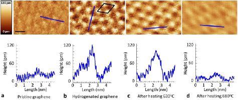
Figure 13. Hydrogenation of graphene on SiC(0 0 0 1). STM topography (top row) and height profiles (bottom row) measured along the blue lines shown in the top panels. (a) Pristine graphene (b) after 5 s of hydrogen exposure (c) after annealing for 5 min at 903 K and (d) after annealing for 5 min at 953 K. Diamond in (b) is the unit cell of the quasi-6 × 6 superstructure that graphene form on this substrate. Reproduced with permission from Goler et al (2013). Copyright 2013 American Chemical Society.
Download figure:
Standard image High-resolution image5.3. Role of the supporting substrate
5.3.1. Bilayer graphene and graphite.
Single layer- (SL), bilayer- (BL) and few layer- (FL) graphene are known to have different electronic structures, that differ also from that of graphite (Castro Neto et al 2009). Nevertheless, it is often assumed that they are all very similar to each other from a chemical point of view, since the interaction between layer is so a small fraction of the H–graphene interaction that it hardly modifies the physics of the adsorption process. As mentioned in the introduction we too made such an assumption in this manuscript and often used graphite as a graphene knockoff, when data on graphene were unavailable. It is thus important to address this issue in detail, and highlight the differences between free-standing SL graphene and graphene interacting with one or more graphene layers.
Apart from the role of curvature discussed above, one key issue in this context is the strength of the interaction between the layers, i.e. the binding energy in BL and/or one of the several (slightly different) interlayer-interaction energies that can be defined in multilayer graphene/graphite. The binding energy in BLG is not experimentally known, but its value is bound from above by the interlayer cohesive energy of graphite—the energy needed to separate the layers, over the total number of C atoms—that was determined to be 52 ± 5 meV/atom (Zacharia et al 2004). Plane-wave vdW-inclusive DFT calculations indicate that the graphite cohesive energy is ca. 10% larger than the binding energy in BLG (see below), so additional layers have a minor importance. In the situation we are interested in, such interlayer interaction represents a restoring force opposing to the surface puckering that accompanies H adsorption, hence it is expected to reduce the hydrogen binding energy when going from SLG to BLG, FLG and graphite. Furthermore, depending on the layer stacking it may also break the sublattice symmetry. In the typical situation of an AB stacking, it determines a 'chemisorption sublattice imbalance' already in BLG, since it acts differently depending on whether the H atom adsorbs on the 'softer' β site (the sites without a C underneath) or on the 'stiffer' α site (the sites with a C underneath). This has led to the fascinating hypothesis that a transient sublattice imbalance (hence a transient magnetization) can be realized when thermally desorbing hydrogen atoms from BL- and ML- graphene (Moaied et al 2015).
DFT calculations with vdW-inclusive functionals, properly corrected for the BSSE if necessary, reproduce the available experimental data on the interlayer interactions rather well and can thus reliably predict the energetics for hydrogen adsorption (Bonfanti and Martinazzo 2018). Table 1 gives some significant energies (in meV per atom) in BLG and graphite, as obtained with two different vdW-inclusive density functionals, vdW-DF (Dion et al 2004, Kong et al 2009) and vdW-VV (Vydrov and Van Voorhis 2010). As can be seen from the table, the two functionals perform similarly well for the interlayer interaction, but the second turns out to be superior when investigating H adsorption (Bonfanti and Martinazzo 2018). The resulting chemisorption energy on SLG is larger than the values it takes on BLG, in agreement with expectations and experimental observations. The reduction of binding energy when passing from SLG to BLG compares favorably with the interlayer interaction energy (per atom), as it should since this is the energy lost by the binding carbon atom when it is pulled out of the surface in the adsorption process. The site-dependency of the chemisorption energy turns out to be smaller, of the order of some tens of meV.
Table 1. Some significant energies (in meV per atom) in BLG and graphite, as obtained with two different vdW-inclusive density functionals (vdW-DF and vdW-VV) using a plane-waves set and the experimental lattice parameters of graphite. EBLG is the binding energy in bilayer graphene, whereas Ecoh, Eex and Ecle are, respectively, the interlayer cohesive energy, the exfoliation energy and the cleavage energy of graphite. See Bonfanti and Martinazzo (2018) for details.
| Method | EBLG | Ecoh | Eex | Ecle |
|---|---|---|---|---|
| vdW-DF | 46 | 51 | 51 | 58 |
| vdW-VV | 47 | 54 | 54 | 62 |
It is worth stressing at this point that addressing vdW interactions is yet challenging nowadays from a theoretical point of view. It is true that recent, vdW-inclusive density functionals can achieve impressive performances, but their reliability is not yet general, and needs to be checked on a case-by-case basis. A common problem that is becoming more and more frequent, though, is the use of the vdW-inclusive functionals in conjunction with an atomic-orbital-based DFT approach, a rather dangerous mix that is largely overbinding because of the basis set superposition error. In the case of H on graphene, for instance, this overestimation of the vdW interactions may completely wash the sticking barrier (Moaied et al 2015, Brihuega and Yndurain 2018), clearly at odds with the many evidences brought above on its existence and its consequences.
On the experimental side, higher reactivity of SL towards hydrogenation (w.r.t. to ML graphene) has been reported by several authors, using different hydrogen sources and graphene supports (e.g. Ryu et al (2008), Elias et al (2009) and Zhang et al (2016)) though opposite findings have also reported (Luo et al 2009). This suggests that, in practice, the preference for SL graphene is probably subtle and can be reverted by changing the operation conditions (e.g. the H atom source).
5.3.2. Metal substrates.
Graphene has been grown on a huge number of metal substrates (Wintterlin and Bocquet 2009, Tetlow et al 2014, Dedkov and Voloshina 2015), either by surface segregation or deposition of hydrocarbons. Perfectly ordered (although often misaligned) epitaxial overlayers can be obtained on a number of hexagonally close-packed surfaces, where Moiré structures with large periodicities appear, as a consequence of a small lattice mismatch between graphene and the underlying metal. The metal–graphene spacings can vary in a wide range between 2.1 and 3.8 Å depending on the strength of the interaction between the carbon sheet and the substrate, that also reflects on the graphene electronic properties. In some systems the  bands are significantly hybridized with the metal band structure. In other systems graphene is quasi free-standing and displays an almost intact electronic structure. Hydrogenation of the carbon sheet can then be performed in different chemical environments, depending on the specific metal susbtrate chosen. Reviewing the literature on such a topic is well beyond the aims of the present work. Rather, in the following, we use a few examples that illustrate the situations typically found in practice.
Depending on the extent of the graphene–metal interactions, we may distinguish four different 'classes'. In a first, graphene is and remains weakly bound to the substrate, even upon extensive hydrogenation. This is rather similar to hydrogenating free-standing graphene, with little (if any) effect of the underlying metal substrate. In a second class fall those combinations where the graphene overlayer is initially quasi free-standing, but shows an increased interaction with the metal substrate upon hydrogen adsorption. A third class is for those combinations where graphene is and remains strongly bound to the surface, while a fourth (apparently yet empty) is for graphene layers that are initially strongly bound to the metal substrate but progressively freed from it as hydrogenation proceeds. Clearly, the progress of the hydrogenation process, as well as the ordered structures that hydrogen can form, may vary largely depending on the graphene-substrate interactions, both 'early' and 'late'. The simplest thing to consider, for instance, is to what extent the induced magnetic moment of a H adatom gets quenched by the substrate, since this determines whether orienting effects innate in the carbon sheet are to be expected or it is the substrate that plays a primary role in the arrangement of the adatoms.
'Graphene on gold' belongs to the first class. Graphene binds strongly on Ni(1 1 1) but intercalation of Au progressively reduces its interaction. 1 ML of Au entirely decouples the carbon sheet from the substrate and makes it quasi free standing and undoped (Varykhalov et al 2008). Angle-resolved photoemission spectroscopy revealed indeed a gapless linear π-band dispersion near K and a Dirac point within 25 meV to the Fermi level. In addition, the Au layer underneath the carbon sheet provides a chemical inert buffer layer that prevents 'late' interactions with the susbtrate upon functionalization. This makes Gr/Au/Ni(1 1 1) an ideal system where investigating hydrogen reactivity (Haberer et al 2010, 2011a, 2011b). Several controlled hydrogenation experiments have been conducted on such system, and saturation values of 25% observed. Furthermore, kinetic experiments have been also performed with both hydrogen and deuterium, and deuteration has been found to proceed faster than hydrogenation, and to lead to substantially higher saturation coverages of 35% (Paris et al 2013).
Ir(1 1 1) is a substrate which couples weakly to the graphene sheet, as evidenced by the presence of characteristic Dirac cones in the quasi particle spectra (Pletikosić et al 2009). Graphene lays at  Å above the metal (Busse et al 2011), and it is only weakly corrugated (Hämäläinen et al 2013), with a variation of its height of
  Å over the ∼25 Å periodicity of the Moiré pattern that originates from the 10% lattice mismatch with Ir(1 1 1) (see figures 14(a) and (b)). Graphene reactivity though varies over the surface. In the so-called hcp and fcc areas of the Moiré, where the position of every second carbon atom coincides with the position of an Ir atom below (see figure 14(d)), the graphene lattice can distort upon hydrogen functionalization, and bind stronger to the metal. This is already clear with a single hydrogen atom (see figure 14(c)) and becomes more plausible when multiple hydrogenation is considered, since a configuration is possible in which every second C atom binds to the underlying Ir, while neighboring C atoms bind to H atoms on top. A selective functionalization of hcp areas by hot H atoms has been achieved and seen to give rise to highly ordered hydrogenated structures, including the opening of a gap in the electronic band structure (Balog et al 2010, 2013, Jørgensen et al 2016). Graphene/Ir(1 1 1) is interesting in many respects, as it has been recently shown that the carbon sheet can 'mediate' the catalytic activity of the substrate, and make dissociative adsorption of H2 feasible when employing vibrationally excited molecules (Kyhl et al 2018). In this case, functionalization of the graphene surface occurs in a highly ordered manner and exhibits an avalanche effect where the first dissociative adsorption event decreases the barriers for subsequent dissociative adsorption.

Figure 14. The structure of the graphene/Ir(1 1 1) Moiré. (a) AFM topography showing the variation of the C atom heights over the Moiré unit cell (reprinted figure with permission from Hämäläinen et al 2013). Copyright 2013 by the American Physical Society. (b) Cross section of the topography in (a) cut along the white dashed line (green), alongside the results of a DFT structural optimization (red symbols) (Martinazzo 2014)). (c) Close-up of the hcp region. Yellow, orange and red balls are for Ir of the first, second and third layer respectively. (d) Side view of the structure that a H atom forms when it is adsorbed in the hcp region (from DFT calculations, (Martinazzo 2014)).
Download figure:
Standard image High-resolution imageFinally, graphene/Ni(1 1 1) represents a case of strong interaction between the carbon sheet and the substrate. This and similar other systems have long been investigated in surface science, where they were found to exhibit a high crystalline quality and inertness in air (Gamo et al 1997). On Ni(1 1 1) a downshift of the Dirac point occurs that causes the hybridization of the graphene π bands with the Ni 3d states. As a consequence, the original electronic structure of graphene at low energy is fully destroyed. Despite this, graphene on Ni(1 1 1) is essentially flat, and lies at about 2.1 Å above the surface (Gamo et al 1997). It forms a 1 × 1 overlayer with two inequivalent carbon atoms, one on top of a Ni atom and one on a hollow site20. Similarly to the case discussed above, the structural changes upon functionalization favor C–H formation on the carbon atoms located on the hollow sites, since in this way the neighboring carbon atoms at top sites buckle downward and increase the strength of the carbon-substrate bonds (Andersen et al 2012). This structural change also affects the adsorption of the subsequent hydrogen atoms, and meta dimers become favored over 'traditional' AB structures. Increasing the coverage, the half-hydrogenation of graphene with full occupation of one sublattice only becomes possible. This is the so-called 'graphone' that has been recently synthetized on Ni(1 1 1) (Zhao et al 2015).
5.3.3. Substrate-induced patterned adsorption and gap opening.
The presence of a metallic susbtrate beneath the carbon sheet allows modulation of the chemical properties, and selective functionalization (hydrogenation) of specific area of the graphene sheet becomes possible. The realization of such patterned hydrogenation is of great technological interest, especially in relation to the long-standing issue of a band gap-opening. That such modulation is indeed operative was shown by Balog et al (2010) on the graphene/Ir(1 1 1) system discussed in the previous section. The authors of Balog et al (2010) were able to hydrogenate the hcp and fcc regions of the Moiré and to open a sizable bandgap in graphene (⩾0.5 eV) by effectively confining the charge carriers in a 'antidot' structure. The approach was later refined (Balog et al 2013), up to the point where selective hydrogenation of the hcp regions only was achieved by controlling the surface temperature during the hydrogenation (Jørgensen et al 2016).
Graphene/Au/Ni too has been shown to give rise to well ordered structures and a gap opening ⩾0.5 eV in graphene (Haberer et al 2010, 2011b). Furthermore, a crystalline compound with 4:1 stoichiometry ('C4H') was apparently realized (Haberer et al 2011a) that is the hydrogen analogue of the single-sided fluorinated product obtained from graphene on Cu(1 1 1) (Robinson et al 2010). These structures are the simplest of a general class of graphene superlattices where a band gap opens because of the preservation of symmetry (Martinazzo et al 2010). Such superlattices have sizable gaps that scale optimally with the superlattice constant, and, in addition, preserve Dirac carriers at the gap edges.
We further notice that patterned adsorption can also be obtained via appropriate treatment of the graphene surface. For example ordered lines of hydrogen dimers have been obtained on graphite upon pre-covering the surface with cyanuric acid (Nilsson et al 2012). The highly stable ordered hydrogenated domains can be exploited to confine electrons similarly to nanoribbons and to realize chemical electron waveguides, as demonstrated by transport calculations (Achilli et al 2014).
6. Outlook
In this work we attempted to give a glimpse of the many facets of the adsorption process of hydrogen atoms on graphene. We highlighted key aspect that seem to be well understood, and attempted to point out those other aspects that, in our opinion, need further investigations. Here, we briefly list the latter (more or less in the same order they appear in the manuscript) in the hope that this can stimulate further work and settle open issues in the field.
The barrier to sticking has been seen to play a primary role in the adsorption process and in the formation of dimers and clusters on the surface. However, it is not yet known with precision, and further work is necessary on this issue from both a theoretical and an experimental point of view. For, on the one hand, current functionals that can be used in condensed matter systems are not accurate enough to describe formation of localized bonds as C–H and, on the other hand, measurements of the initial sticking coefficient for H under carefully controlled conditions have not been yet undertaken.
Transport measurements under carefully controlled coverage conditions are desired to establish the role that adatoms like hydrogen atoms might play in limiting the mobility of charge carriers in graphene. But also, theoretical modeling at more realistic distributions of adatoms (i.e. that account for dimer and cluster formation) is required to fully understand the role that H atoms might play in triggering transitions between different transport regimes. In principle, clustering of H atoms should convert the strong, resonant scattering centers into more common short-range scatterers with smaller effects on carrier mobility. Hence, starting from a low coverage condition, an 'anomalous' transition should occur at increasing coverages that just reflects the onset of dimerization. However, no study exists at present that addresses this issue.
Ordering of adatoms remains a long-standing goal in the search for magnetism on carbon based materials. Manipulation of the adatoms (and full control over their position) has been shown possible with the tip of an STM on a microscopic region, but viable routes for applications are yet to be uncovered. The chemical modulation provided by the support on which graphene is grown is a promising approach, though efforts are yet required to decouple the functionalized graphene from the substrate. Similar issues concern the modification of the electronic properties of graphene, and in particular the band-gap opening much desired for logic applications. In this context, crystalline hydrogenated graphene with 1:1 stoichiometry has been not yet realized, while the fluorinated analog seems to be realized.
The high reactivity of the edges is generally accepted, but not yet experimentally proved for single layer graphene. Likewise, the subtle differences in the single-, double- and multi-layer graphene and the role of curvature and substrate interactions need yet further investigation.
We believe that a combined experimental and theoretical effort on the above issues may progress our understanding of the interactions between hydrogen and graphene, improve our ability to control graphene's properties and be useful for the many other functionalization approaches that have been developed since the first isolation of graphene.
Acknowledgments
MB gratefully acknowledges fellowship support by the Alexander von Humboldt Foundation. RM acknowledges Università degli Studi di Milano for supporting this research through the project "PSR2017-Linea 2-Azione B".
Footnotes
- 5
Ivanoskaya et al performed a full geometrical optimization including the lattice size. Such a strategy is surely correct when applied to a periodic arrangement of H atoms, but it is clearly questionable when the aim is to investigate a single H adatom on the surface.
- 6
As mentioned in the introduction, early attempts date back to 1969 but little characterization of the surface was possible at that time (Beitel 1969).
- 7
To be specific, we mean a reduced description that can handle a reasonable number of degrees of freedom in a non-Markovian setting.
- 8
It determines, through the average frequency spacing, the Poincaré recurrence time of the system beyond which the Hamiltonian dynamics departs from that of the GLE. For the problems discussed below some tens of oscillators are enough for the dynamics of interest to be over before the first recurrence sets in.
- 9
It is understood that the zero energy level is that of an isolated pZ orbital, that is also the Fermi level when graphene is charge neutral.
- 10
More precisely, this number is the dimension of a specific irreducible representation of the symmetric group, and it is given by
 for N electrons with total spin S.
 - 11
In the following λ is understood to be
, where is a real energy and . - 12
Here
stands for , P being the projector onto the primary subspace. - 13
These are 'oriented' because of the asymmetric atomic arrangement with respect to the impurity site.
- 14
This comprises the spin and the valley degeneracy factor appropriate for graphene.
- 15
That is when the substrate is aged long enough in a hydrogen atmosphere at a given pressure.
- 16
This raises the possibility of singlet states with 'unpaired' electrons, so called open-shell singlets. Notable examples are zig-zag nanoribbons, where unpaired electrons appear at the edges because of a (local) imbalance, in the absence of a global imbalance.
- 17
When H is a second quantized Hamiltonian a further projection onto the single particle space is required. Notice further that the same results follow upon partitioning the one-electron problem similarly to what has been done in section 2.5, but now using the A subspace as primary space.
- 18
Edge sites with Z = 3 are best considered as bulk sites, since they have three π bonds like the C atoms in the bulk.
- 19
In fact, the reaction proceeds through the following steps: (i) formation of solvated electrons (from Li into liquid NH3), (ii) e attachment to the graphene sheet to form a radical anion and (iii) double protonation in the quenching step (addition of water or an alcohol).
- 20
This is the so-called top-fcc structure. A second, top-bridge configuration is possible that is slightly less favored.


