

Abstract
In this note we introduce a hierarchy of phase spaces for static friction, which give a graphical way to systematically quantify the directional dependence in static friction via subregions of the phase spaces. We experimentally plot these subregions to obtain phenomenological descriptions for static friction in various examples where the macroscopic shape of the object affects the frictional response. The phase spaces have the universal property that for any experiment in which a given object is put on a substrate fashioned from a chosen material with a specified nature of contact, the frictional behaviour can be read off from a uniquely determined classifying map on the control space of the experiment which takes values in the appropriate phase space.
Export citation and abstract BibTeX RIS
A large class of many body systems ranging from dense colloidal suspensions, granular matter to vortex matter in superconductors makes dynamical transitions between stuck and moving states under the influence of an applied force [1–4]. The transition that takes the system from a stuck to a moving state is usually referred to as yielding or depinning and this is associated with microscopic plastic processes [1]. Similarly, the transition that takes a system from the moving (flowing) to a static state is referred to as jamming, and is marked by a drop in the single particle mobility [5]. The problem of the motion of a single object has been studied earlier from the point of view of the underlying microscopic mechanism of elastic instability [6–9] and plasticity [10, 11]. In this paper we re-visit the phenomenology of onset and cessation of motion of a single object which is frictionally coupled to a substrate, and geometrically classify the various phases associated with it and the transitions between them, in terms of subregions of appropriately chosen phase spaces.
Figure 1(a) shows a schematic representation of the experimental setup to measure friction between an object and the substrate where N is the applied normal force and F is the applied tangential force. The point of application of F is kept low enough so as to minimise the toppling torques. Depending on the force of static friction, such an object will either remain stuck, or begin to move under the applied force F. Correspondingly, we can say that the object is in a stuck phase or in a slip phase. If we keep all other parameters constant, the maximum value of  for which the object remains fixed is called the coefficient of static friction, denoted by
  . Suppose now a tangent force F is applied to an object as above, which drives the object at a steady velocity v. It is known that for moderate values v and of
  , the ratio
  is independent of
  . The plot of
  against the velocity v continues as the well known Stribeck curve. The red curve in figure 1 is a schematic representation of this curve, which is a plot of
  versus v ([12]). It consists of all possible pairs
  for which the object can be driven at a fixed velocity v for a moderate
  . A static object (
 ) remains stationary if
  . The force of friction drops as the object starts to move, and its magnitude decreases from higher values to a lower steady value
  for a certain range of velocities, beginning with a velocity v0. The resulting curve is flat in a small interval starting from
  , where the value of
  is
is  . The exact shape of the curve between 0 and v is not known as it is a region of intermittent response. The Stribeck curve has portions of negative slope, and these are regions of instability. For if the slope is negative at a point
  , and the value of
  is kept steady, then any slight increase in velocity will lead to an acceleration, and any slight decrease in the velocity will lead to a deceleration, which will get further enhanced as long as we are in the part of the curve with negative slope.
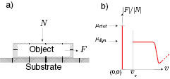
Figure 1. (a) A schematic representation of the experimental setup to measure friction between an object and the substrate where N is the applied normal force and F is the applied tangential force. The point of application of F is kept low enough so as to minimise the toppling torques. (b) A schematic representation of the Stribeck curve and the velocity gap v0.
Download figure:
Standard image High-resolution imageNote that by definition of  , the vertical portion of the
  axis up to the point
  lies on the Stribeck curve. The Stribeck curve has a horizontal portion (where
  is independent of v) starting from a small non-zero velocity v0. We call v0 as the velocity gap. The corresponding value of
  is known as the coefficient of dynamic friction, and it is denoted by
  . It is known that
  , and for
  , the Stribeck curve does not have any noticable portions of continuity with positive or zero slopes. The inequality
  means that if we apply a small mechanical disturbance to an object in the stuck phase (
 and
and  ) to momentarily dislodge it, so as to allow the object to begin moving under the applied force F with a speed
  , then there are two possibilities. For
  , the object rapidly comes to a halt again, while for
  , the object continues to move. As
  , the portion of the Stribeck curve which lies over
  must have portions of negative slope or discontinuities. The resulting unstable behavior of the object makes a precise plot of the Stribeck curve difficult in this region. The presence of discontinuities and regions of negative slope above
  mean that if in the above we have
  and
and  , then the object either rapidly comes to a halt or speeds up, or shows an intermittent behavior mixing the above two possibilities.
We will say that a stuck object is in a strongly stuck phase or a weakly stuck phase, depending respectively on whether the object comes back to a halt or continues moving after being subjected to a momentary disturbance with velocity  as above. As the Stribeck curves becomes approximately horizontal for a small interval after v0 [13] there is a comfortable margin for v1, which make the definitions of these phases robust. If the disturbance given to a weakly stuck object is so small as to give it a velocity
  , then the response will be intermittent
The above discussion was focused on a 1-dimension situation, where a given object is moving on a given homogeneous substrate by translational motion in a given direction. If the object or substrate are not isotropic, the phases will depend on directional parameters, and the quantities  and
and  will not be constant but will depended on multiple parameters [14–16]. In this paper we study the geometric phenomenology of the above phases with multi-parametric dependencies for a given pair of object and substrate with a given nature of contact. We set up an appropriate phase space X together with nested subregions
  , where points of X parametrize the magnitudes of the forces on the stationary object and the angles between the force F and fiducial directions on the object and the substrate, the subset
  corresponds to those values for which the object is in a stuck phase, and the even smaller subset
  corresponds to those values for which the object is in a strongly stuck phase. Note that the set
  corresponds to the slip phase, and
  corresponds to the weakly stuck phase.
In the classical Coulomb regime of static friction, the phase regions  and
and  turn out to determined by single numbers
  (the coefficient of static friction) and
  (the coefficient of dynamic friction). However, beyond the Coulomb regime, the regions
  and
and  become more complicated functions of the magnitude
  of the normal force and the angles between the force F and fiducial directions on the object and the substrate. (We will leave out for simplicity the dependence of static friction on the contact time, as in [17, 18].) We show that the shapes of these regions can depend on the macroscopic shape of the object, in particular, on its edges and corners.
The triples  , which are associated with a given object, substrate and a fixed nature of contact (this last notion is explained later), have a certain universal property. Namely, given any experimental setting for friction, with a space S of control parameters, there is a unique map ψ from S to X, such that the object with control parameters given by a point
  is in a certain phase if and only if its image
  is in the corresponding subregion of X. The phase space
  for the given object, substrate and nature of contact is characterized by this universal property. The map
  will be called as the classifying map for the experiment. We illustrate these concepts with some experiments.
Phase spaces for friction and their coordinate descriptions
For the basic experiment with static friction, let there be chosen a pair of orthogonal directions on the object. We place the object on the substrate in any manner in which the first of these directions is normal to the substrate. The second chosen direction on the object, which is therefore tangent to the substrate, will be called as the fiducial direction on the object. Let there be also chosen a fiducial direction on the substrate, which is tangent to its surface. Note that these two fiducial directions and the applied force F are coplanar, as all three are tangent to the surface. The choice of the fiducial directions on the object and the substrate matter exactly when both the object and the substrate are nonisotropic. In this case, let  denote the angle from the fiducial direction on the object to the fiducial direction on the substrate. Let
  and
and  respectively denote the angle between the applied force F and the fiducial direction on the object or on the substrate. Unlike ϕ, the angles
  and
and  are indeterminate when
  . When
  , we have the equality
  . We will always assume that N is non-zero, which is physically justified by the presence of gravity and adhesion in our actual experiments, and so
  , the open positive half line. As F is allowed to be zero, the ratio
  lies in the closed positive real half-line
  . As the coordinates
  and
and  are angular coordinates, their values correspond to points on the circle S1. As the value of
  is indeterminate when
  , that copy of S1 gets squeezed to a point. Hence, for a given value of
  , the pairs
  form a plane E2 with polar coordinates
  , where
  and
and  . Hence, the 4-tuples
  form the space
  , which is a 4-manifold diffeomorphic to
  .
.
There are various simpler situations, where the object or the substrate or both are isotropic, or where we limit  to a range of moderate values, in which instead of the 4-dimensional space X4, we can work with smaller 3-dimensional spaces Y3,
  , X3, or 2-dimensional spaces EI, E2,
  , or the half-line
  , as we now describe. All these spaces are sub-quotients of X4. Their interrelationships are depicted as a cubical lattice of spaces in figure 2. The arrows stand for projection maps which have a simple coordinate description in coordinate terms. These spaces which are discussed in details below have the following coordinate description.
  ,
,  ,
, 
 ,
,  ,
, 
 ,
,  ,
,  ,
,  .
.

Figure 2. The figure shows a lattice whose vertices are various spaces that are underlying spaces X for a possible phase space  for friction. The arrows are the forgetful projection maps (they omits certain information) between them. The four maps shown by black arrows leave out the magnitude
  of the normal force. The four blue maps forget
  by leaving out the coordinate ϕ or the coordinate
  as the case may be. The four parallel red maps forget
  by leaving out the coordinate
  or by replacing the pair of numbers
  by the single number
  , as the case may be.
Download figure:
Standard image High-resolution imageThe space X3: If we fix (or omit) the value of  , then the triples
  are points of
  . Topologically, this space can be visualized as an open solid torus in
  . Alternatively, we can view it as
  with the last coordinate being periodic with period
  , as the circle S1 can be viewed as a line
  with a periodic coordinate. The figure 3 schematically shows the way of visualizing X3 as a solid torus, and depicts a subregion
  within it.
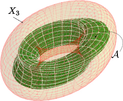
Figure 3. The yellowish solid torus depicts the space X3, which is the phase space when both the object and the substrate are anisotropic, and when  is moderate. The darker greenish region is a schematic representation of the region
  for a hypothetical object and substrate.
Download figure:
Standard image High-resolution imageThe spaces Y3 and  : If the object is anisotropic but the substrate is isotropic, then the angle
  can be ignored, and so we get the space
  with coordinates
  , which is a 3-manifold diffeomorphic to
  . Similarly, if the object is isotropic but the substrate is anisotropic, we get a space
  , with coordinates
  which is diffeomorphic to Y3 with
  .
.
The spaces E2 and  : If we fix (or omit)
  , and if the substrate is isotropic, so that we can ignore ϕ and
  , then the remaining data is in the form of pairs
  , which gives a point (in polar coordinates) of the plane E2. Similarly, if we fix (or omit)
  , and if the object is isotropic, then we get pairs
  , which form a plane
  . The spaces E2 and
  are both diffeomorphic to
  .
.
The space EI: If both the object and the substrate are isotropic, then the coordinates  and
and  in X4 can be ignored. In this case, we need to only consider the pairs
  , which form the 2-dimensional space
  , which is the first quadrant in
  with the boundary
  removed.
The half line  : If we fix (or omit)
  , and if both the object and the substrate are isotropic so that we can forget both
  and ϕ, then we are left with only a single non-negative real number
  , which is a point of the closed half line
  . In geometric terms, this is the conventional Coulomb scenario in which the frictional response is characterized by a single number.
In coordinate terms, the maps  ,
,  and
and  in the commutative diagram in figure 2 respectively send the 4-tuple
  to the 3-tuples
  ,
,  and
and  . The other arrows have similar obvious coordinate descriptions.
The classic experiment shows that there exists a region  within X4, such that if
  then the object remains stationary. We will call
  as the sticky region. This geometric representation raises a natural question: what is the shape the sticky region
  ? In particular, one can ask: how does the shape of the object affect the shape of the region
  ? In this paper, we mainly explore the phenomenology of the relationship between these two shapes. We will also consider experiments in which one or more of the object and substrate are isotropic, and in this cases we will replace X4 by a smaller space X3, Y3,
  , E2,
, E2,  , EI or
  as appropriate, and define a sticky region
  in it similarly.
The partition 

It is known that the force of friction sharply decreases when a stationary object is set in motion (e.g. see p 144 of [19]). Consequently, a smaller applied force is sufficient to sustain motion, compared to what is needed to initiate motion. This geometrically results in a partition of the sticky region  into two subregions
  and
and  , as follows. Consider a point
  of
of  . This physically corresponds to the situation where steady forces F and N are applied to the stationary object, which leave the object stationary. To this stationary object, on which the steady forces F and N are acting as above, we give a burst of random mechanical vibrations which momentarily dislodges the object so that it commences to move under the force F, acquiring a minimum velocity v0 (the value of
  may depend on the directional parameters
  , but as the Stribeck curve flattens from
  for a small interval, the below definitions of
  and
and  are robust). Alternatively, the burst of vibrations may be administered to the substrate to set the object in motion. As explained in the beginning, now there are two possibilities. Either the object continues to move for some time, in which case we say that
  , or the object rapidly comes to a permanent halt in which case we say that
  . If the disturbance resulted in an initial velocity less than v0, the object will rapidly come to a halt if in
  , while it will show intermittent behaviour if in
  . This fact allows a test for determining whether a point is in
  or
or  without knowing the value of v0, however, as the Stribeck curve is nearly flat for some velocity range from v0. This phenomenon, of the velocity rapidly going to zero once it drops below a critical value v0, was described by the term velocity gap in [20]. This partitions
  into two subregions
  and
and  . In case we have a fixed or a moderate value of
  , or one or both of the object and the substrate are isotropic, we replace X4 by the appropriate lowest dimensional space among X3, Y3, E2 etc shown in figure 2, and define analogously the decomposition
  within this smaller dimensional space.
The triple  is the phase space for a frictional experiment, in a precise universal sense, as we explain later. In case the object or substrate are isotropic or
  can be left out, the phase space will be the one of the triples
  etc, where the parameter space is the smallest, instead of
  . When this happens, the regions
  and
and  in X4 etc will be the inverse image of the universal regions
  and
and  in the phase space, under the projection arrows shown in figure 2.
Diagrammatic representation of Coulomb friction
Phrased this way, the Coulomb laws for static friction can be interpreted to say that the region  is defined in Y3 by a single inequality
  in terms of a constant
  which depends only on the nature of the surfaces of the object and the substrate. Similarly, the region
  is defined in Y3 by a single inequality
  where
where  depends only on the nature of the surfaces of the object and the substrate. The inequality
  always holds. In particular, the shape of the object does not affect the shapes of
  and
and  . This implies that the angle
  is not relevant (for the original object placed with a new angle
  can be regarded as a new object with the same kind of surface). These laws are known to be valid experimentally when
  is not too large (what actually matters is that the resulting maximum pressure exerted at any point of the interface is not too large, see pp 19–20 of [10]).
The figure 4 schematically depicts the regions  and
and  in Y3 in the Coulomb scenario. These look like coaxial solid circular cylinders with radii
  for small
  . Thus, for the Coulomb scenario, the phase space
  is the triple where
  ,
,  and
and  . When
  becomes very large, we move out of the Coulomb scenario, i.e. the ratio
  is no longer constant. Under the influence of a large normal force, the object begins to adhere to the substrate, which increases the radii of both
  and
and  with
with  . The upper part of figure 4 schematically shows such an increase, where for simplicity, we have retained the rotational symmetry of
  and
and  . Assuming such a rotational symmetry indeed holds, we must take
  , while the regions
  and
and  will have to be experimentally determined.
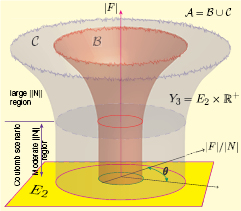
Figure 4. The regions  ,
,  and
and  with variable
  in the space
  with coordinates
  . As
. As  increases these regions become broader. For simplicity we have retained rotational symmetry of these regions even for large
  .
.
Download figure:
Standard image High-resolution imageA thought experiment beyond the Coulomb scenario
In the laboratory experiments that we discuss later in the paper, we take  to be in the moderate range, so that the object does not adhere to the surface and the frictional force is linear in
  . Hence in this range, we can ignore the coordinate
  , and just retain
  . Assuming moreover that the substrate is isotropic, so that ϕ and
  can be ignored, we can work in the 2-dimensional space E2 with polar coordinates
  , and take our regions
  and
and  to be defined inside this space E2, which was introduced earlier.
In contrast to the Coulomb scenario, we will show that when an object is placed on a substrate which is significantly rougher than the object, then the regions  and
and  may depend on the shape of the object. Conversely, if the object is rougher and the substrate is smoother, then this effect disappears. Before giving experimental data which shows this effect, we present a simple idealization of the object and the substrate, for which one may see how the regions
  and
and  are influenced by the macroscopic shape of the object. In this idealization, both the object and the substrate are fashioned from cobblestone material [21]. This kind of material is made by embedding rounded cobblestones of nearly identical sizes in an elastic material. At the exposed surface of this material, we assume that at least half of each exposed cobblestone is embedded in the elastic material, which holds the cobblestones together. We assume that the typical distance of closest approach between two adjacent cobblestones is approximately the same as the diameter of a cobblestone. This distance
  defines a characteristic length scale associated with the object. The magnified view in figure 5 shows sheets made from two such materials which have different values of
  . More complicated models of cobblestone materials will have a denser packing, or will have the interstices filled with smaller stones and so on, and there will be multiple length scales associated with the material, but for simplicity, we will work with our model material which has a single length scale
  .
.
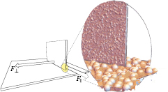
Figure 5. The figure shows a schematic representation of a thought experiment described in the text using cobblestone materials.
Download figure:
Standard image High-resolution imageWe assume that the material of the cobblestone as well as the elastic material have a common non-zero coefficient of static friction against any of these two materials. Assuming different values for the possible coefficients, though more realistic, will not make a qualitative difference to the outcome of the following.
We now describe a thought-experiment in which an object in the form of a thin sheet fashioned from cobblestone material with length scale  is placed on a substrate fashioned from cobblestone material with length scale
  , such that
  and
and  are significantly different, with
  . The object is assumed to be thin in the sense that the thickness of the sheet from which it is fashioned is significantly smaller than the characteristic length scale
  associated with the substrate. However, the breadth and length of the object (unlike the thickness of the object) are assumed to be orders of magnitude larger than the sizes of the cobblestones. This is depicted in the magnified view within figure 5, with the thin sheet perpendicular to the substrate. It can be seen that the vertical thin sheet gets partially embedded in the gaps of the cobblestones of the substrate. For this to happen, the elasticity of the sheet comes into play, allowing it to bend slightly to fit better in the valleys between the protruding cobblestones of the substrate (in contrast, a completely rigid sheet will rest itself on just a few of the cobblestones and the edge will not get embedded into the gaps between the cobblestones of the substrate). In order to move laterally under the force
  , the sheet has to climb over each of a larger number of such protrusions to begin its motion, compared with what it has to do in order to move longitudinally under the force
  . The thinness and the elasticity of the sheet, which allows it to bend, comes into play when it moves longitudinally, allowing it to navigate by threading through the gaps between the cobblestones, so that it needs to climb only over a smaller number of them. Our assumption, that the thickness of the sheet from which the object is fashioned is significantly smaller than the characteristic length scale
  associated with the substrate, is crucial here. If the rectangular sheet has its corner clipped, so as to present a rounded corner, with its radius of curvature greater than the characteristic length
  of the substrate, then the longitudinal motion in the direction of the rounded corner becomes even easier, compared with longitudinal motion when the corner is sharp. We call the phenomenon of extra frictional response due to a leading sharp corner of the object as the corner effect. So long as there is a leading corner, such an effect will show itself even if the sheet is not perpendicular to the substrate. The difficulty of moving laterally increases with the length of the sheet, as its edge has to climb over a greater number of cobblestones on the substrate. We call this phenomenon as the edge effect.
For the edge effect to manifest itself, the edge should be sharp at a scale of the order of the scale of granularity of the substrate—a more rounded 'edge' will not show this effect. As a result of the edge effect, the region  becomes broadened in the direction perpendicular to the edge, to an extent which depends on the length of the edge.
Instead of the sheet being perpendicular to the substrate, we can consider an arrangement where it has an acute angle α. In this case, the motion of the sheet in the forward direction will be more difficult than its motion in the opposite direction. An extreme example of this is when the angle α is 0, that is, the object is a sheet is lying on the substrate. To isolate the effect of the leading edge, we will assume that the object is fashioned out of a rectangular sheet, and the opposite edge is raised by curling upwards (see figure 6(a), and also figure 7(b)). Such an object will have have a smaller friction moving in the direction of the curled edge, and much higher friction moving in the direction of the straight edge.
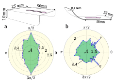
Figure 6. The figure shows the measured effects of edges and corners on the region  in two experiments, in which a paper sledge and a curled paper sheet were placed on a grit paper substrate. We used
  thick bond paper for fashioning both the sledge and the curled sheet, and used a P180 silicon carbide grit paper with average spacing between grit particles of the order of
  as the substrate. 'The fiducial vectors on the objects are depicted as arrows drawn on them. The sledge in (a), made by bending a paper sheet, has rounded corers on its blades to lessen the corner effect. The blades give rise to a prominent edge effect, as the edges are vertical to the substrate. The paper sheet in (b) is curled at one end, so that it has corners only on one side. The edge effect for a horizontally resting sheet is not strong as its edge does not get much embedded into the substrate. The points P and Q demonstrate existence of the corner effect, due the physical corners at either end of the leading edge of the curled paper. In both these figures, because of the presence of noise, the data points are shown to be just inside the schematic plots of the corresponding regions.
Download figure:
Standard image High-resolution image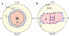
Figure 7. (a) The figure shows the empirically plotted regions  (blue) and
  (red) of
  for a square plastic block (sides
  , height
  ). In spite of the absence of circular symmetry in the block, the regions are approximately circular, showing that corner and edge effects are negligible in this case. (b) The figure shows the motion onset curve
  (blue),the subregion
  (blue) and
  (red) of
  for a sledge placed on a neoprene sheet. The sledge is made by gluing surgical blades to opposite sides of a square plastic block (length
  , height
  ). In both these figures, the data points in blue are shown to be just inside the schematic plots of the corresponding regions, while the data points in red are just outside the region
  .
.
Download figure:
Standard image High-resolution imageThe nature of the contact between the leading edge of the object and the substrate in this experiment will depend on the extent of the rigidity of the object. Given that the macroscopic dimension of the object is several orders of magnitude greater than  , the object will remain almost flat and its leading edge will remain almost straight, but it will get stuck against the most protruding of cobblestones from the substrate. This will lead to greater resistance to move in the direction of any leading straight edge.
Though the actual materials involved are not cobblestone materials, the idea behind the above thought experiment gets realized in the experiment performed by placing a curled paper sheet on a rougher substrate, described later.
There is another scenario where a similar effect of the edge becomes manifest. This involves a block placed on substrate made of cobblestone material such that the substrate is elastic, and the block is smoother than the substrate. The substrate develops a depression because of the force N on the object, and once again, any motion of the block transverse to an edge of it, or in the direction of a sharp corner of it, encounters the protruding cobblestones of the substrate as obstructions. This leads again to an edge effect or a corner effect on the resulting regions  and
and  , which get broadened in the direction perpendicular to an edge or in the direction of a corner. Consequently, for an object with prominent corners and edges, the shape of the region
  , instead of being a circular disk in E2 centred at the origin as in the Coulomb scenario, will come to depend on the shape of the object. For an object with no sharp corners, if the ratio

goes to zero, then the Coulomb scenario will get restored. These edge effect scuffs the material and produces scratches on the surface [22]. The corner effect is accompanied by large stress concentrations, as a result the contacting objects dig into one another which produces tear [23].
The laboratory experiments
We can now say that the classic table top experiment will produce a constant  , that is, a region
  as in the lower (moderate
  ) part of figure 4, under the following assumptions: (a) the surface of the object is made of an isotropic material, (b) the surface of the substrate is made of an isotropic material, (c) the edge effects are negligible, (d) the corner effects are negligible, (e) the toppling torque produced by the force F is negligible (this is achieved if the point of application of F is low enough – a counterexample is given by rolling motion) and (f) the magnitude of N is not too large.
We are interested in finding the frictional response, more precisely, in finding the shapes of the regions  and
and  , when some of the above assumptions (except (f), which we will not violate) are transcended. As we are leaving out the magnitude
  (and retaining just
  ), we can work in one of the spaces X3, E2,
  or
or  according to the below table, and define the regions
  and
and  in this space.
| Anisotropic substrate | Isotropic substrate | |
|---|---|---|
| Anisotropic object | X3 | E2 |
| Isotropic object |  |
 |
For this, we use two different experimental arrangements, which respectively use as the substrate an inclined plane or the inner surface of a slowly rotating hollow horizontal cylinder.
When the substrate is an inclined plane, the forces F and N are supplied by gravity, with  where α is the inclination of the plane. We assume that we are in the realm of moderate
  even when the plane is horizontal so that
  is at its maximum. We note that
  corresponds to a horizontal plane, and
  corresponds to a vertical plane. Therefore,
  is the angle between the chosen fiducial vector on the object and the downward direction on the inclined plane. We vary
  by rotating the object around an axis perpendicular to the substrate. The height of the object is kept small compared to its lateral dimensions whenever we want the toppling torque produced by F to be negligible. If one needs to test a non-isotropic substrate using this apparatus, this is possible by holding the angle
  to be constant as α is slowly varied, and then repeating the experiment for a new value of
  . The angle of inclination α of the plane is mechanically increased slowly, at the rate of approximately 50 degree per hour, starting with
  . For different chosen values of
  , note was made of the value of α at which the object began to move. This gave various data points with polar coordinates
  in
in  , close to its boundary
  (the onset curve), which enabled a schematic plot of the region
  .
.
This arrangement is used to plot the region  in E2 (with coordinates
  as described above), for different objects. If the object placed on the inclined plane is a circular disk and moreover the substrate is isotropic, it is clear by symmetry that the region
  is the circular disk centred at the origin
  of E2 with radius
  , and the onset curve
  is its boundary circle
  . If the object is not circular, there is no a priori reason for the onset curve to be a circle as above, and the actual shape of it must be measured experimentally.
The figures 6, 7 and 8(a) show the observations and the plotted onset curves for (1) a paper sledge on a grit paper, (2) a paper curled on one side on grit paper, (3) a plastic square block placed on a glass plate, (4) a sledge with metallic blades placed on a neoprene sheet and (5) a dumbbell placed on an glass plate. To minimize the toppling torque on the non-rolling objects (cases (1)–(4) above), their height was kept small compared to their lateral dimensions.
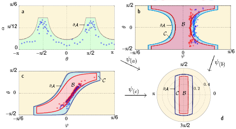
Figure 8. The panels (a)–(c) show the plots for the onset curves for a dumbbell in terms of the control parameters for the inclined plane apparatus, horizontal cylinder apparatus and tilted cylinder apparatus. These onset curves are the pull backs under the respective classifying maps  ,
,  and
and  of the universal onset curve in the phase space E2 associated with a dumbbell on a glass substrate, shown in panel (d) with polar coordinates
  .
.
Download figure:
Standard image High-resolution imageTo plot the region  , the plane was first kept inclined at various fixed values of the angle α at which the object remained stationary, and then a small burst of mechanical noise was imparted to the assembly, and its effect was observed. Note was made of whether the resulting motion of the object was transient or was a sustained movement. These observations approximately gave the boundary
  and so led to a schematic plot of region
  (see figure 7). This experiment was done for a square block and a metal sledge. (The paper sledge and the plastic dumbbell, being too light, were not convenient for the administration of a mechanical burst, as they often got thrown off by the noise.)
The second experimental arrangement, namely, a rotating hollow horizontal cylinder, was used to plot the regions  and
and  and the onset curve
  for a dumbbell (see figure 8(b)). In this experiment a hollow glass cylinder (radius
  ) whose axis is horizontal is rotated very slowly around its axis (at an angular velocity ≈
 radians
  ). A dumbbell made of plastic (radius of the balls
  , length of the dumbbell
  ) is placed at different angles (values of
  ) at the lowermost point on the interior surface of the cylinder, and its subsequent motion is observed. As the radius of the cylinder is much larger than the size of the object placed on its surface, the surface can be regarded as approximately flat at the scale of the object. In any experiment with the cylinder apparatus, care must be taken that the nature of contact between the object and the cylindrical surface is similar to that between the object and a flat surface, which is possible for rolling objects such as balls or dumbbells.
Some of the advantages of using the cylinder apparatus over using an inclined plane are the following. (i) The slope of the cylinder continuously changes from 0 to 
 . This makes it possible to test the frictional behaviour of an object placed on the cylinder for all values of the slope of the substrate. (ii) At the lowest part of the horizontal cylinder (along the line
  ) any stationary object defines a point in the region
  , as it remains stationary even after a small disturbance. The slow rotation of the cylinder, which has a very low noise level, enables us to slowly transport (without imparting a significant amount of linear momentum) a small object placed at
  to a region with a higher slope while being stationary w.r.t. the substrate, from where it begins to move down. This allows the determination of the boundary
  . (iii) As the object moves down, the slope of the substrate goes to zero, and the object comes to a stop. The point where it comes to rest is in the region
  , but not precisely on the boundary
  , because of the downward momentum of the moving object. Similarly, the presence of the mechanical noise of rotation allows the object to penetrate a bit into
  instead of stopping just at its boundary. These effects being stochastic, observing the points where it stops thus enables an approximate conservative determination of the boundary
  of region
  . So instead of a sharp boundary, as expected from the existence of the velocity gap mentioned earlier, we get a fuzzy boundary in the experiment. (iv) The rotation of the cylinder does not change the geometry of the experimental setup. The gentle rotation allows us to put bounds on the regions
  and
and  without resorting to a sudden burst of mechanical noise (as in the inclined plane experiment where it is more difficult to control and has a pronounced destabilizing effect on an object which can roll, such as a dumbbell).
The limitation of a cylindrical substrate is that while we can put balls or dumbbells on it, where the nature of the contact is very similar to that for a flat substrate, we cannot put blocks with flat faces on a cylindrical substrate without drastically altering the nature of the contact. Given the advantages and disadvantages of each, one or both the experimental set ups were deployed as were appropriate.
Results and discussion
Square block in the Coulomb scenario
When a square block is placed on an inclined plane, the experiment gives the expected results in the Coulomb scenario when the block has a low height (to minimize the toppling torque, which would have accentuated the edge effect by putting extra pressure along the leading edge) and has rounded edges or has a sufficiently large size (so that the ratio of the perimeter to area is small, making edge effects negligible). The regions  and
and  are measured to be concentric circular disks centred at the origin and the onset curve
  is a circle, in spite of the lack of rotational symmetry in the shape of the block. In fact, this property of isotropy of the frictional response will hold for any shaped block of large enough size whose perimeter is not too jagged, so that the ratio of edge length to area is small.
This can be seen from the following argument: Consider a flat, irregularly shaped object with piecewise smooth outer boundary for which we assume that the ratio of the area of the object to the perimeter of the object is small, and whose boundary is not 'too jagged'. Such an object is schematically shown (in yellow) in figure 9. A tangent force F is applied in two different directions in parts figure 9(a) and (b) of the figure. Let the object be approximated by a union of squares joined together, oriented according to the direction of the applied force. As the size of the squares is made arbitrarily small, the area of object gets approximated by the total area of the squares to any desired precision. At the same time, the outer perimeter of the assembly of squares approximates the perimeter of the block within a factor of  (a factor which comes from the worst case scenario of approximating an edge at an angle of
  to the direction of F). Hence if the ratio of the area of the object to the perimeter of the object is small, then the ratio of the total area of the assembly of squares to the outer perimeter of the assembly of squares is again small. The imaginary edges of the squares which are glued to each other have no physical existence, and hence they have no effect on the friction. This implies that the two assemblies of squares, and hence the object, have the same frictional response in figures 9(a) and (b).

Figure 9. The figure schematically represents a rigid body with two different reconstructions of its shape via conjoined square blocks, suited to the two different directions of the applied force F shown in panels (a) and (b).
Download figure:
Standard image High-resolution imageCurled paper sheet, and paper sledge, on a grit surface
The experiments described in figure 6 are realizations of the thought experiments. The flat end of the paper shows greater resistance to onset of motion as compared to the curled edge, which is a manifestation of the edge effect, as expected. As expected from the thought experiment, the paper sledge on the grit paper moves most easily in the direction of its long axis, and with greatest difficulty in the sideways direction.
Viscoelastic version of edge effect
A variation on the above experiment is where the sledge is made by gluing surgical blades to the opposite sides of a plastic block is placed on a deformable substrate made from neoprene (see figure 7(b)). These materials are not in the domain of the thought experiment, which was with cobblestone materials. However, deformations of a viscoelastic substrate and their propagation lead to corner and edge effects much like those discussed in the thought experiment. This follows from the dependence of the reaction force of a viscoelastic material on the deformation rate [24], and the fact that the deformation is confined to a band around the edge with width equal to the characteristic length scale s associated with the mechanical deformation of the body or the substrate. In this set up, the edge effect becomes prominent when the ratio of the area of the contact region between the body and the substrate to the perimeter of the region of contact (this ratio has the dimension of length) is of the smaller than the length scale s. Conversely, if the ratio

goes to zero, then the Coulomb scenario will get restored provided that the time rate of change of force is kept small (no sudden jerks are applied) to keep the viscous reaction negligible. An edge effect of the above kind was indeed shown by the metallic sledge on the neoprene substrate (see figure 7(b)).
Dumbbell
A dumbbell, made by joining two balls, can roll under a torque. In this case, the regions  and
and  in E2 are determined by four constants
  , with
  . The definition and significance of these constants is explained in the Appendix A of [20]. The region
  can be described as follows. Let
  . A point
  with
with  or
or  lies in
  if
if  . A point
  with
with  or
or  lies in
  if
if  . The theoretical expectation for the shape of the region
  is given by replacing the static coefficients by their dynamic counterparts, and correspondingly replacing the constant
  . The experimental plots of
  (made with an inclined plane as well as a rotating cylinder) and the plot of
  (made with a rotating cylinder), are consistent with the above for moderate values of θ. On the other hand, a moving dumbbell for which θ is close to
  (which therefore slides more than it rolls) tends to change its value of
  towards 0 or π as it slows down because of the torque produced by differential normal and tangent forces on the two balls as well as due to mechanical irregularities. Consequently, our experimental plots of the regions
  and
and  in figure 8 are not closed when θ is close to
  ). Noise (produced by the apparatus which raises the plane or rotates the cylinder) is constantly present in the experiments, so a dumbbell begins to move when it is somewhere within the region
  , instead of starting from a point of
  . The momentum of the moving dumbbell leads to its stopping somewhere inside the region
  , instead of stopping exactly on crossing
  .
.
Universal property of the phase spaces of friction
Consider any experimental arrangement, in which a chosen object O is pressed against a surface made with material M, with a normal force N and subjected to a tangent force F, which may depend on the configuration of the object (its position and placement on the surface). We do not need to assume that the surface is flat, but we must require that the nature of the contact between the object and the surface is of a chosen sort (the figure 10 explicates with an example the concept of the 'nature of the contact'). Suppose that the surface is homogeneous, but not necessarily isotropic. If it is not isotropic, let a unit tangent vector field V on the surface encode the possible directionality of the substrate (no such V is to be given if the surface is isotropic). Let there be fixed a fiducial vector on the object. Then from the control parameter space S of the object, we get a classifying map  to the phase space X4 which sends a point of S to the data
  for the configuration given by that point. If the surface is isotropic, we instead consider a map to Y3. If we leave out
  we get a map to X3, etc. The phase spaces, together with their regions
  and
and  , have the universal property that under the classifying map ψ, the inverse images of
  and
and  are the corresponding empirically determinable regions in the control parameter space S, where the object is in the stuck phase, and in the strongly stuck phase, respectively.
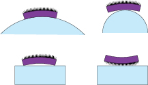
Figure 10. Examples of different natures of contact. The four panels of this figure schematically show an object O coloured purple resting on different substrates made from the same material M coloured blue, such that the nature of contact is different in each panel. Therefore, there will be four different phase spaces  for these arrangements, in which the underlying space X will be the same but the
  's and
  's will change.
Download figure:
Standard image High-resolution image
Examples of the above for three different experiments with a dumbbell are given in Figure 8. where the panels figures 8(a)–(c) show the plots for the onset curved for a dumbbell in terms of the control parameters for three different experimental arrangements. These onset curves are the pull backs under the respective classifying maps  ,
,  and
and  of the universal onset curve in the phase space E2 associated with a dumbbell on a glass substrate, shown in panel figure 8(d) with polar coordinates
  . Inclined plane apparatus: the figure in panel figure 8(a) shows the region
  plotted for a dumbbell placed on an inclined plane, in terms of the control parameters α and θ. The map
  is given by
  and
and  . Horizontal cylinder apparatus: the figure in panel figure 8(b) shows the regions
  and
and  plotted for a dumbbell placed on the inner surface of a horizontal cylinder apparatus, in terms of the control parameters φ and θ. The map
  is given by
  and
and  . Tilted cylinder apparatus: the figure in panel figure 8(c) shows the regions
  and
and  plotted for a dumbbell placed on the inner surface of a tilted cylinder apparatus in terms of the control parameters φ and θ. The tilt of the cylinder from the horizontal is fixed at
  . The map
  is given by
  and
and  . In figure 8(a), the plotted data points in blue are inside
  , while in figures 8(b) and (c), the blue points are inside
  while the red points are inside
  . To plot
  we used
  and
and  . Similarly, to plot
  we used
  and
and  .
.
In other words, once we know by experimenting (say, by using an inclined plane) the regions  and
and  in the phase space, the corresponding regions
  and
and  in any other experimental set-up (whose control parameter space is S) can just be read off from the regions in the phase space by using the classifying map
  without once again performing the experiments in the new arrangement. Thus, we can get the regions
  and
and  for any experimental arrangement from the universal regions
  and
and  in phase space, by simply determining the classifying map to the appropriate space. This is what is meant by the universal property of these spaces X4 etc as phase spaces of friction.
When the object O and the material M (and the nature of contact) are altered, we will get new regions  and
and  even if X remains the same, giving a new phase space
  .
.
It is possible to extend the construction of phase spaces of friction together with their universal subregions, which will have a universal property, to experiments with composite objects, where the object has multiple parts which are joined by hinges, springs, etc. We can also increase the dimension of X to incorporate the effect of ageing of contact, as well as to incorporate a continuously variable nature contact. Also note that the classifying map  to the phase space X preserves the symmetries of the experimental set-up, that is, symmetries of S, and so it descends to a map
  on the quotient space
  of S by the group G of all symmetries of the experimental set-up. This was used above for the experiment with an inclined plane (where there is an action of
  by translation) and for a cylinder (where there is an action of
  by translation along the axis), and what we have actually depicted in figure 8 are the respective maps
  .
.