

Abstract
The goal of atomic force microscopy (AFM) is to measure the short-range forces that act between the tip and the surface. The signal recorded, however, includes long-range forces that are often an unwanted background. Lateral force microscopy (LFM) is a branch of AFM in which a component of force perpendicular to the surface normal is measured. If we consider the interaction between tip and sample in terms of forces, which have both direction and magnitude, then we can make a very simple yet profound observation: over a flat surface, long-range forces that do not yield topographic contrast have no lateral component. Short-range interactions, on the other hand, do. Although contact-mode is the most common LFM technique, true non-contact AFM techniques can be applied to perform LFM without the tip depressing upon the sample. Non-contact lateral force microscopy (nc-LFM) is therefore ideal to study short-range forces of interest. One of the first applications of nc-LFM was the study of non-contact friction. A similar setup is used in magnetic resonance force microscopy to detect spin flipping. More recently, nc-LFM has been used as a true microscopy technique to systems unsuitable for normal force microscopy.
Export citation and abstract BibTeX RIS
1. Introduction
Lateral force microscopy (LFM) is a technique which was pioneered to study friction, and later developed as a microscopy technique in its own right. Similar to atomic force microscopy (AFM), a sharp tip is brought close to a surface, and the force interaction is measured. There are many cases in which measurements of the lateral component of force, especially dynamic measurements, yield greater signals of small interaction forces. In order to properly appreciate non-contact lateral force microscopy (nc-LFM), this review will start with a brief history of its development, beginning with the scanning tunneling microscope (STM). The invention of AFM and its subsequent progress led to true non-contact techniques being developed. Non-contact techniques were also brought to LFM, allowing measurements of lateral forces before the tip is in contact with the surface.
The second section of this article is a review of two areas to which nc-LFM has been applied. The first is non-contact friction. Before contact is made between two bodies, they can already exert a frictional force upon each other. A second area is spin sensitivity. As nc-LFM is not sensitive to background forces with large vertical components, it is better suited for small in-plane signals, sketched in figure 1.
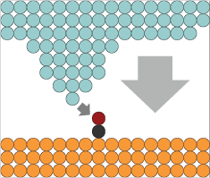
Figure 1. Long-range forces (larger arrow) can dominate the AFM signal and are typically in the direction of the surface normal, whereas short-range interactions (smaller arrow) have a strong lateral component.
Download figure:
Standard image High-resolution imageIn the third section, the use of nc-LFM as a microscopy technique is discussed, starting from the first use of LFM to observe atomic features on a surface. That same year, the first observation of every atom of a surface was made. Soon after, it was clear that small amplitudes were required to clearly resolve individual atoms. Finally, applications of nc-LFM are presented: a vertically soft but laterally stiff material is imaged; friction anisotropy is measured at the atomic level; and the lateral bending of a single molecule is measured.
1.1. From STM to non-contact force microscopy
At the beginning of the 1980's, a group working at IBM in Zürich was developing a method for characterizing electronic components with high spatial resolution. The idea was to use a sharp metal tip over a sample, apply a voltage between the tip and sample, and to record the resulting current as a measure of its properties on a local scale. Control over the tip-sample distance was so accurate that the group was able to move the tip close enough to observe a current resulting from the quantum tunneling effect [9]. Binnig and Rohrer called their new microscope the scanning tunneling microscope [7, 8]. We now understand the current to be a local measure of the density of states between the Fermi level and the applied voltage (e.g. [16, 75]).
In order for the tunneling current to be measured, the tip must be close (typically less than 1 nm) to the sample. At this distance, several phenomena exert substantial forces. Electrostatic interaction between the tip and sample, separated by vacuum or a dielectric, is attractive. The long-range van der Waals interaction is also attractive. Chemical bonding is a general term in the field of AFM used to describe the interaction between the individual atoms of the tip and the nearest surface atoms, including van der Waals attraction between the two followed by formation of a chemical bond and Pauli repulsion. The question arose as to what role these forces played on STM measurements, and how they could be measured.
In 1986, Dürig, Gimzewski and Pohl, inspired by previous work of Israelachvili and Taylor [38], proposed a method for using the STM to measure forces [20]. The sample was mounted on a relatively soft cantilever (a spring constant of  N
N  at the end), sketched in figure 2(A). At room temperature, it oscillated with a thermal amplitude around
  pm. Interaction between the tip and sample can be thought of as the addition of a second spring to the system with spring constant kts. kts is also called the force gradient. For force measurements sensitive to the vertical component of force, Fz,
  . This additional spring shifts the resonance frequency, which could be measured by acquiring a power spectrum of the current. Although I will first present AFM and its development, this measurement technique is at the heart of non-contact force microscopy: the tip-sample interaction acts as an additional spring and a change in oscillation frequency is a measure of force.
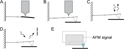
Figure 2. Schematic methods of local force detection (A) STM measurements of the thermal oscillation of a cantilevered sample, after Dürig and co-workers, [20]. (B) An STM used to measure cantilever deflection. A tip, mounted to the cantilever, probes the sample locally. After Binnig and co-workers, [6]. (C) Optical interferometry to detect the cantilever deflection, as described in [55]. (D) Optical reflection, in which the reflected beam is detected by a two-quadrant detector, after Meyer and Amer, [59]. (E) The qPlus sensor, invented by Giessibl, is a stiff quartz sensor whose oscillation is detected electrically, [29].
Download figure:
Standard image High-resolution imageIn parallel, a technique was developed to directly measure forces via Hooke's Law. In 1986, Binnig filed a patent for the atomic force microscope [10] and along with Quate and Gerber, published the first paper describing atomic force microscopy [6]. They proposed mounting a tip at the end of a cantilever with a known spring constant k and measuring the deflection  directly via a STM tip behind the cantilever, sketched in figure 2(B). This was not the first experiment in which forces between a sharp tip and a surface were measured (e.g. [67]) but it was the first to propose the idea of measuring forces between individual atoms to map out a surface. In doing so, a new field was born. Not only did AFM allow non-conductive samples to be probed, but (quoting from Dürig and co-workers), 'in contrast to tunneling, where only electrons with momentum... near the Fermi surface, contribute appreciably to the tunnel current, interaction forces involve electrons in total k space' [20].
There are many technological developments in the field of force microscopy. I have selected a few here such that the reader will have a technological background for the non-contact LFM measurements presented in this review. These developments can be characterised into two: detection methods and operational modes. From the initial proposal to use an STM tip to detect the cantilever deflection, optical and electrical detection methods are predominantly in use.
In 1987, Martin, Williams and Wickramasinghe published a paper summarizing two advancements for AFM: use of optical detection to monitor the cantilever's position and the use of dynamic AFM [55]. The optical detection was a laser interferometer, and the setup is sketched in figure 2(C). As discussed by McClelland, Erlandsson and Chiang, optical measurements are less sensitive to thermal drift and the roughness of the cantilever's backside [57], making detection more reliable and easier than with an STM tip.
Soon thereafter, in 1988, Meyer and Amer proposed reflecting a laser beam off the back of the cantilever and detecting it with a position-sensitive detector [59], sketched in figure 2(D). This position-sensitive detector is typically a two cell detector. In 1990, they expanded on this proposal and asserted that by expanding to four cells arranged in a  matrix, torsional modes could simultaneously be detected [60].
In 1998, almost ten years later, Giessibl invented a new AFM sensor, called the qPlus sensor, in an effort to optimize measurements with atomic resolution. The qPlus sensor is based upon a quartz tuning fork (the original design was based on tuning forks that were commonly used for wrist watches) [29]. The piezoelectric effect drives a current as it oscillates which can be electrically detected, sketched in figure 2(E). It is also much stiffer than a typical sensor. Instead of a spring constant around  N
N  , the qPlus sensor has a stiffness of 1800 N
  . While this high stiffness makes static deflection measurements difficult, the qPlus sensor is specifically designed to operate with small amplitudes in a dynamic mode.
As well as the detection methods being improved, new operational modes were accessible for AFM measurements. Binnig and co-workers initially proposed contact-mode AFM in which the tip scratches over the surface [6], much like a needle of a record player. Atomic resolution was later demonstrated in contact-mode (e.g. [31]) but the main challenge is to keep the tip atomically sharp and well-defined while substantial vertical and lateral forces are acting upon it. One way around this problem is to move from contact-mode to dynamic-mode measurements. Instead of pressing down on the surface, the tip is driven to oscillate, and characteristics of this oscillation change as the tip interacts with the surface. It's important to note that not all dynamic modes are non-contact modes. One of the most common dynamic modes involves the use of an amplitude setpoint smaller than the free-resonance amplitude to control the tip-sample distance. The tip is driven to oscillate near its resonance frequency at a given drive amplitude, and touches the surface (decreasing the amplitude) during each oscillation cycle. Extracting forces from this method is challenging and typically requires assumptions being made about the tip-sample contact [3] or about its motion [36]. Indeed it is still a very active field of research to extract tip-sample forces when the tip makes intermittent contact with the surface (e.g. [26]). True non-contact techniques, however, allow the surface to be measured without a force pressing down on it.
Similar to Dürig and co-workers, Martin and co-workers describe a dynamic non-contact technique [55]. Instead of measuring the resonance frequency, however, they measure the amplitude. They oscillated the tip at a constant drive frequency and drive amplitude, and measured the resulting amplitude of oscillation. The damping of the cantilever's oscillation is described in terms of the quality factor Q. The lower the Q value, the broader the spectral peak at the resonance frequency will be. Interaction with the surface will shift the centre of the peak and therefore by recording the amplitude of oscillation, they can measure kts. This method is only reasonable for systems with relatively high damping (low Q), because the spectral peak needs to be relatively wide.
In 1990, Albrecht, Grütter, Horne and Rugar proposed frequency-modulation atomic force microscopy (FM-AFM) in order to take advantage of cantilevers with a larger Q value [2]. The key is to make use of a phase lock loop (PLL) to follow the resonance frequency f and drive the cantilever at that frequency. [21] is a good review of the underlying mathematics and control hardware required.
The measured quantity in FM-AFM is the frequency shift  , which relates to the tip-sample interaction via the equation:

Here, f0 is the unperturbed resonance frequency. This equation is valid so long as kts is constant over the oscillation of the tip, an assumption referred to as the small-amplitude approximation.
For an AFM tip oscillating in the vertical direction, kts is the gradient of the vertical component of force. In order to convert  into force, kts must be integrated along a vertical path from a point where
  N (that is, a point sufficiently far from the surface). In the case of a conservative force field, the force can then be integrated to yield the potential energy.
If the small-amplitude approximation is not valid, the cantilever motion must be explicitly taken into account [19, 28, 30]. To summarize the final result, a similar expression to equation (1) is derived where a new parameter,  is introduced in place of
  .
.  is called the weighted force gradient, and takes into account the oscillation of the cantilever. The calculation of kts from
  is called deconvolution. The two most common deconvolution methods are the Sader–Jarvis method [69] and the Giessibl matrix method [30].
In FM-AFM, the amplitude of the oscillation is kept constant by a second controller, working in parallel to the PLL. If the interaction with the sample is conservative, then the only energy dissipation will be via the cantilever, and the magnitude of the drive signal will remain constant during measurements. Additional damping will require a larger drive signal, which can be recorded to evaluate dissipative interactions.
1.2. Application of normal-force FM-AFM to the measurement of lateral forces
Consider a dataset that maps  as a function of both a lateral coordinate, x, and the vertical coordinate z, sketched in figure 3(A). At each x position, the z spectrum can be evaluated to yield the vertical component of force, sketched in figure 3(B). A subsequent integration will yield the potential energy U. A derivative of the potential energy in the x direction then yields the lateral component of the total force, sketched in figure 3(C).

Figure 3. Using nc-AFM to evaluate lateral forces. (A) A AFM tip, oscillating vertically, records a  map, approaching the adsorbate until it moves. (B) At each x position, the vertical component of force, Fz is evaluated. From Fz, the potential energy map
  is derived. (C) A derivative of U at constant height z can be used to evaluate the x component of force, Fx.
Download figure:
Standard image High-resolution imageThis method was used by Ternes, Lutz, Hirjibehedin, Giessibl and Heinrich to measure the force required to push an atom along a surface [74]. In 1990, Eigler and Schweizer showed that an STM tip could be used to re-arrange atoms on a surface (Xe atoms on an Ni surface, spelling the iconic IBM logo) [22]. Ternes and co-workers used nc-AFM to evaluate the lateral forces up to the point at which a Co atom and a CO molecule moved on a surface. They collected  data in both z and x, starting from a position far from the surface and then approaching until the adsorbate moved. They then evaluated lateral and vertical forces just before the motion. The maximum lateral force they recorded before hopping was dependent both upon the adsorbate and the surface: a single Co atom on Pt(1 1 1) required 210 pN, whereas Co on Cu(1 1 1) required only 17 pN. A single CO molecule on Cu(1 1 1) required 160 pN. This was the first real look into the forces at play during atomic manipulation.
Mao, Chen and Xue then performed the same analysis to evaluate the lateral force required to move a phthalocyanine-based molecule (H2Pc) on a Pb surface [53]. H2Pc is a much larger planar molecule which self-assembles to form islands on the surface. When H2Pc is part of an island, the lateral force required to move it away from the island is 37 pN, which is much higher than the 12 pN required to move it when it is isolated on the surface. This is a beautiful demonstration of the lowering of potential energy that comes with island formation of certain adsorbates.
Langewisch, Falter, Fuchs and Schiermeisen performed a similar investigation of PTCDA on a Ag surface [51]. In this investigation, the authors pay careful attention to the complimentary channels of both vertical force and dissipation. They find that the interaction between the tip and molecule needs to be in the repulsive regime to move the molecule. They also find that, in this case, the vertical forces cannot explain the lateral manipulation and that they observe motion of the molecule only when a lateral force of 190 pN is applied. They report a dissipation of approximately 25 meV/cycle, before the molecule moves, indicating that the oscillating tip might be exciting the molecule and easing its lateral manipulation.
Emmrich, Schneiderbauer, Huber, Weymouth, Okabayashi and Giessibl went back to the work of Ternes and co-workers, repeating the manipulation of CO molecules on a Cu surface with atomically-characterized tips [24]. By imaging a CO molecule, known to be an inert probe, we acquired an inverse image of the tip shape [23, 78]. We found that the lateral force required to move the CO molecule was different for different tip apeces. One conclusion we drew was that the potential energy surface of the CO molecule is not simply a linear superposition of the potential energy of the tip and the surface, but rather that the tip weakens the Cu-CO bond, modifying the potential energy landscape of the surface. Surprisingly, we found that tips with larger attractive vertical force components also required greater lateral forces before the CO molecule would move. One explanation is that as CO is known to adsorb preferentially on adatoms and step edges as opposed to flat terraces, it is possible that a sharper tip with less overall van der Waals attraction weakens the Cu-CO bond and facilitates lateral manipulation.
Outside of lateral manipulation, nc-AFM has been used to evaluate lateral forces above surfaces and adsorbates. Acquiring the necessary three-dimensional dataset is time-consuming and thermal drift must be accounted for. For these reasons, as well as the necessary tip stability, these measurements are very challenging at room temperature, and more often conducted at low temperature (liquid He temperatures). Albers and co-workers describe how to accomodate for this and evaluate the lateral force component above a graphite surface [1]. Neu, Moll, Gross, Meyer, Giessibl and Repp proposed a method of evaluating the lateral forces to correct for tip deformation [63], a topic which will be discussed in more detail in section 3.5.
Work with FM-AFM has also been used to advance contact-mode lateral force measurements. The concept with these measurements is to use FM-AFM to construct a well-defined tip and then to slide the tip over the surface, recording the frequency shift as a function of position. Pawlak, Ouyang, Filippov, Kalikhman–Razvozov, Kawai, Glatzel, Gnecco, Baratoff, Zheng, Hod, Urbakh and Meyer examined the FM-AFM signal of a single porphyrin molecule being dragged over a clear copper surface [65], sketched in figure 4(A). The drag pattern, shown in figure 4(B), is very similar to the pattern observed in contact-mode LFM [56] (discussed in section 1.3), but Pawlak and co-workers can be sure that they are sliding over the surface with a well-defined apex. Modelling the tip-sample interaction, they use the FM-AFM signal to yield information about the frictional response of the system. One of the major challenges of this investigation is to determine the orientation of the molecule, which the authors determine with the help of DFT modelling. Similar to the work of Langewisch and co-workers [51], this study concludes that the internal degrees of freedom of an individual molecule play a major role in the tribological properties.
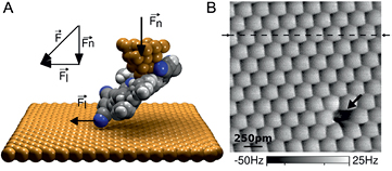
Figure 4. By picking up a well-defined adsorbate, nc-AFM measurements can be used in contact mode to measure friction. (A) A porhyrin molecule picked up by a metal tip dragging along a surface. (B) The drag pattern with atomic resolution and a single atom defect. Reprinted with permission from [65]. Copyright 2016 American Chemical Society.
Download figure:
Standard image High-resolution imageA year later (2016), Kawai, Benassi, Gnecco, Söde, Pawlak, Feng, Müllen, Passerone, Pignedoli, Ruffieux, Fasel and Meyer performed a similar experiment sliding graphene nanoribbons over a gold surface [41]. They used molecular precursors to grow atomically-precise graphene nanoribbons on the surface [12] and characterized them with STM. First they performed a similar analysis as that of Ternes et al, determining the lateral force required to move the nanoribbon as a function of length. Then they brought the tip close to one end, lifted a fraction of the nanoribbon off the surface, and recorded  as the tip dragged over the surface. They interpret their data with a molecular mechanics model in which the Au–C interaction is given by a Lennard–Jones potential. This model reproduced the low friction ('almost frictionless sliding') of the nanoribbon.
A tip oscillating vertically above a surface is not directly sensitive to lateral forces, however nc-AFM measurements have been used to investigate lateral forces. By deconvoluting the  signal and integrating to yield the potential energy, the lateral force between the tip and sample can be evaluated. This has been applied, not only to surfaces and adsorbates, but to determine the lateral forces just before manipulation of atoms and molecules on surfaces. More recently, nc-AFM has been used with a well-characterized tip to investigate contact-mode friction. Although the interpretation of the results is non-trivial, the method is invaluable because the sliding interface can be characterized down to the atomic level. In the next section, direct lateral force measurements are discussed, and the development to dynamic LFM measurements is presented.
1.3. Development of lateral force microscopy
The birth of lateral force microscopy, that is, the direct measurement of lateral forces with an AFM tip, is often attributed to work by Mate, McClelland, Erlandsson and Chiang, published in 1987 [56]. Instead of using optical interferometry reflecting off the top of the cantilever, they measured light reflected off the side of the cantilever, allowing them to be sensitive to the lateral deflection. They recorded lateral forces as the tip moved relative to the sample over a range of speeds and normal (vertical) forces. The authors note that, in accordance with Coulomb's law of friction, the lateral forces are independent of velocity over a range of 4 nm  to 400 nm
  and that the average friction over a surface is approximately linear as a function of the vertical load. Perhaps most interestingly, as they scan the tip over the surface, the map of lateral force has corrugations with the same lateral spacing as the surface atomic periodicity. We saw atomic corrugation in the images taken by Pawlak et al [65], but this came as a surprise to Mate and co-workers. What about an uncontrolled interface would lead to in-phase motion of several atomic contacts that result in a signal with atomic corrugation?
Since its invention, LFM has played a definitive role in the field of nanotribology [5, 17], and many wonderful findings have come of it. Curious readers might want to start with [33], a book edited by Gnecco and Meyer. Here, I summarize a few highlights to put contact-mode LFM in context. Dienwiebel and co-workers measured graphite with a flake of graphene, and showed not only friction anisotropy but indications of superlubricity at various angles [18]. Cannara and co-workers compared deuterium-terminated silicon with hydrogen-terminated silicon and concluded that the various phonon modes have a direct influence on the dissipated energy during friction [14]. Finally, Filleter and co-workers showed that single-layer graphene has much poorer energy dissipation compared to bilayer graphene, and relate this to a difference in electron-phonon coupling, which they confirm via ARPES spectroscopy [25].
We now have all the pieces in place for the inclusion of dynamic AFM techniques to LFM measurements. In 1992, O'Shea, Welland and Rayment applied dynamic LFM to measure the lubricant properties of a surfactant [64]. They used optical measurements to record torsional bending, and oscillated the sample laterally at an amplitude under 5 nm, recording the resulting lock-in signal of the torsional motion. They were sensitive to changes in friction as a function of the normal force. After a critical value, the authors proposed that the surfactant was being pushed away from the tip-sample interface.
A decade later, Marcus, Carpick, Sasaki and Eriksson reported observing a signature of friction in tapping-mode measurements while investigating polymer multilayers [54]. It was known that due to the growth of these polymers, friction was anisotropic over them depending on the direction of their backbone (see, e.g. [15]). In their setup, the tip oscillated at an angle of approximately 11° from the surface normal. They observe contrast in the phase of the image, which they associated to the tip sliding over the surface.
Two years later, in 2004, Huang and Su, inspired by the success of tapping mode AFM, proposed driving the torsional mode of the cantilever and recording amplitude and phase [37]. The authors noticed that their torsional-resolution mode brought much higher sensitivity to atomic steps than is seen in normal tapping-mode AFM images. This increased sensitivity was noted by Yang and Hwang in 2010, who modified the approach slightly to monitor the torsional resonance using the frequency-modulation technique [81]. They reported that the  signal they recorded was only measurable when the tip is close (
 1 nm) to the surface, and that in contrast to the normal force, was a purely monotonic signal. They were able to oscillate at sub-nanometer amplitudes, and reported atomic images of a mica surface as well as an image of DNA on the surface. This monotonic nature of the
  signal is again most likely because the tip was in contact with the surface, but the authors assert one of the two most powerful attributes of LFM: that they are particularly sensitive to short-range interactions because 'the torsional oscillation is not sensitive to the long-range normal interactions.'
Dynamic LFM in contact mode is still being used and developed to investigate friction between two well-defined nanoscale contacts. Mertens, Göddenhenrich and Schirmeisen recorded the anharmonic components of the lateral oscillation of the tip as a function of normal force to probe the transition between static and sliding friction [58]. Krass, Gosvami, Carpick, Müser and Bennewitz investigated hexadecane, used as a model for lubricants, on graphite [47]. More recently, Cai and Yao used dynamic LFM to controllably rub a sample and produce a local triboelectric charge [13].
This work, to merge the popularity of tapping-mode with lateral oscillations, still does not overcome the initial problem with contact-mode AFM or LFM: that the tip-sample interface is poorly defined at the atomic scale, and subject to wear and therefore change. These problems are overcome by moving from a contact or tapping-mode scheme to a true non-contact scheme. In the early 2000's, three applications of nc-LFM started to emerge. The first two, non-contact friction and spin contrast, utilized the high sensitivity of dynamic lateral force measurements to detect small forces but were less concerned with spatially mapping the surface. Direct imaging was the third application, in which the lateral signal is used similar to the non-contact AFM signal, to produce a map of the surface and adsorbates.
2. Non-contact lateral force measurements
The goal of the measurements in this section is to be sensitive to a small tip-sample interaction as the tip moves laterally across the surface. The cantilever can be vertically very stiff, allowing the tip-sample distance to be accurately controlled and reducing the possibility that the attractive surface interaction will cause the tip to jump to the surface (a problem referred to as jump-to-contact in the AFM community). In general, the surface is treated as uniform, and as such, large amplitudes can be used. This reduces noise and allows for different techniques to be used, as discussed in the context of non-contact friction.
2.1. Non-contact friction
Even without direct contact, two bodies moving close to each other can affect a force on one another (see, e.g. [76]). The equation of motion for a tip on a cantilever, in which a frictional term  (proportional to velocity) is included, is

By measuring the cantilever dynamics,  can be determined.
  is a combination of internal damping of the cantilever, which we previously described by the quality factor, and any additional damping term of the surface,
  . These two components can be separated by making one measurement far from the surface and one close to the surface.
Stipe, Mamin, Stowe, Kenny and Rugar built a nc-LFM setup, sketched in figure 5(A), in which a gold tip oscillated laterally over a surface to measure the lateral motion as a function of the vertical tip-sample distance [73]. They performed three complimentary forms of measurement. In the first, they excited the cantilever to an amplitude of approximately 20 nm and let the amplitude decay. Monitoring the ringdown allowed them to calculate the damping. This method works when the ringdown is on a timescale for which the exponential decay of the amplitude can reasonably be probed. The second method was to record the envelope of the thermal vibration for a period of minutes and to compute its autocorrelation. The sampling rate was too slow to record the oscillation of the cantilever, and it is rather the amplitude of the envelope that is measured. As in the work of Dürig et al [20], thermal excitation drives the cantilever, and would be mathematically represented by an additional term in equation (2). Thermally exciting the cantilever also means that the oscillation amplitude is much smaller. The autocorrelation of the envelope decays exponentially proportionally to Q (see, e.g. equations (2) and (15) in [40]). The authors recorded the envelope of the thermal amplitude and computed its correlation. The third method was to measure the thermal spectrum and to evaluate the damping based on the shape of the thermal peak. Interestingly, although they could observe a thermal peak with the tip close to the sample, they were unable to use this method because the peak shape did not represent a harmonic oscillator. The authors propose that a small degree of anharmonicity was enough to distort the curve. Both the ringdown method and the autocorrelation method, however, make it clear that there is a strong dependence of the frictional damping ( ) with respect to the tip-sample distance.

Figure 5. (A) Diagram of the setup used to probe non-contact friction. (B) Relation of the friction parameter  to tip-sample distance over three samples of various resistivity. Reprinted figure with permission from [73], Copyright (2001) by the American Physical Society
Download figure:
Standard image High-resolution imageThe authors use these two methods to probe friction as a function of the applied voltage between tip and sample. There is a parabolic relation between the voltage and the friction, implying a relation to the electric field, suggesting that this weak damping might be caused by currents in the tip and sample that dissipate according to Ohm's law. They take a step further and measure friction over a non-conductive surface, showing again an increase in the friction, as shown in figure 5(B). Gold, with lower resistivity than silica, yields much lower  values and therefore much lower frictional effects.
Kuehn, Loring and Marohn used a similar setup to measure non-contact friction with the ringdown technique [49]. They acquire data over thin layers of polymers deposited on a gold surface. The three different polymer samples have various relative dielectric constants, from  to
to  . Continuing from the work of Stipe and co-workers [73], Kuehn and co-workers investigate non-contact friction as a function of the electric properties of the surface. Non-contact friction increases as a function of
  , and is a function of the thickness of the film. When the film is thinner, the friction is lower. Indeed, the authors even show that if they evaporate a thin layer (40 nm) of gold above the polymer sample, the non-contact friction greatly reduces. The conclusion of this study is that the time-varying electric field is responsible for a restoring force on the tip. In a complementary article they expand upon their theory and compare explicitly the outcome of their model to the data [50]. The reader is directed to the publication for futher details, however the ratio of the friction ratios between various polymers is in good agreement with the data over a small range in which the tip is less than 20 nm from the surface.
In 2011, Kisiel, Gnecco, Gysin, Marot, Rast and Meyer published their investigation of non-contact friction above a niobium surface, taking measurements both above and below the critical temperature of the superconductive phase transition [45]. They used the ringdown technique to evaluate  both as a function of tip-sample distance and applied voltage. As the temperature is lowered past the critical temperature,
  changes abruptly, shown in figure 6(A), clearly showing the effect of the electronic nature on the sample in non-contact friction. As a function of voltage,
  has a very different dependence, based on whether Nb is superconducting or not, shown in figure 6(B). The expected V2 dependence when Nb is in its metallic state supports the proposal that the friction is due to Ohmic losses, whereas the V4 dependence indicates phononic losses. (The theory behind this is discussed in more detail in [77].)
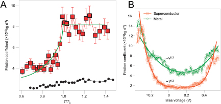
Figure 6. (A) Non-contact friction over Nb while the temperature drops below the superconductive critical temperature TC. (B) The bias dependence of  changes from the metallic to superconducting state, indicating different physical damping mechanisms. Reprinted by permission from Macmillan Publishers Ltd: Nature Materials, [45], copyright (2011).
Download figure:
Standard image High-resolution imageNon-contact lateral force measurements have been instrumental in probing non-contact friction. For a more complete review of non-contact friction, especially in terms of force microscopy, the reader is directed to [46].
2.2. Spin resonance
A second application is in the detection of spin systems. The typical setup is to use a magnetic tip, which creates a non-uniform magnetic field that penetrates into the sample. In addition, a microwave generator drives unpaired spins to resonate at a frequency  . This occurs when the total magnetic field B0 is related to
  via the gyromagnetic ratio γ:

As the cantilever oscillates and the appropriate B0 sweeps through the sample, the spin flips along the axis of magnetisation. More detailed reviews can be found in [48, 72].
In 2003, Mamin, Budakian, Chui and Rugar reported measurements taken above silica, irradiated to create dangling bonds with unpaired electron spins [52]. Rather than the critical value of the magnetic field, B0, existing in a small volume that can be thought of as a point directly under the tip apex, it is more accurate to think of it as a roughly hemispherical shell passing through the sample, shown in figure 7(A). As the tip interacts with the spins, they flip. By leaving the microwave generator off for a half of the cantilever cycle, the spin component will not flip as the tip swings over, sketched in figure 7(B). Turning the microwave generator on again leads to switching of the spins, but now in the opposite direction. The back action on the tip can be detected via a change in the oscillation frequency. The signal from one single flip, however, was too weak to be detected. They therefore omit one half of a cycle at a much lower frequency,  . While they could try to observe this signal via a lock-in amplifier, they look for harmonics at
  in the power spectrum.
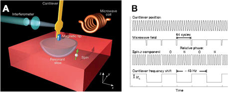
Figure 7. (A) Diagram of the setup used to probe spin. (B) Schematic of the timing diagram for detecting spin flips. Reprinted by permission from Macmillan Publishers Ltd: Nature [68], Copyright (2004).
Download figure:
Standard image High-resolution imageIn their second paper, Rugar, Budakian, Mamin and Chui perform a similar analysis on a sample with a relatively low concentration of dangling bonds. They calculate the mean spacing between spins in the low-density sample to be 200 to 500 nm [68]. They oscillated the tip at an amplitude around 20 nm and scanned the tip over the sample in one direction, finding a very strong spatially localized signal. The authors conclude that the observed signal comes from the flipping of a single electron spin.
In 2004, Jenkins, DeFlores, Allen, Ng, Garner, Kuehn, Dawlaty and Marohn published work on batch fabricating soft cantilevers with a magnetic tip [39]. With nickel as a tip magnet material, they achieved cantilevers with parameters  ,
,  Hz and
  N
N  . Garner, Kuehn, Dawlaty, Jenkins and Marohn use these cantilevers to measure nuclear spins in a GaAs sample [27]. Their setup involves an amplitude
  nm at a tip distance of 160 nm from the surface. The force gradient is applied via excitation of spins in the magnetic field and they detect a frequency shift on the order of tens of milliHertz. Interestingly, the authors claim that their measurements are limited by non-contact friction damping, thus lowering the quality factor of their setup.
3. Non-contact lateral force microscopy
Let us now turn to nc-LFM as a microscopy technique in its own right. A FM-AFM setup in which the tip oscillates along the surface normal vector is directly sensitive to forces along the surface normal. This has many advantages, including being able to detect the surface upon approach. There are two challenges to approaching the surface using the LFM  signal. The first is that the LFM signal is short-range, and therefore requires as very fast reaction by the controller, and the second is that there is no guarantee that the absolute value of the signal will reach a setpoint value, depending upon the point of approach. If, however, STM or the normal bending mode can be used to approach the tip to the surface, a setup where the tip oscillates along the surface can be used. The mathematical description of the frequency shift and its relation to force remains the same: interaction with the surface changes the frequency of oscillation proportional to the force gradient, kts, along the direction of oscillation.
So far, I have reviewed the birth of non-contact lateral force microscopy and its application in two fields, both of which used the experimental setup to detect very subtle tip-sample interactions. In this section, I review articles in which nc-LFM was used as a microscopy technique with an emphasis on works with atomic resolution.
From a technological viewpoint, what are the sensor requirements for atomic resolution with nc-LFM? Small lateral amplitudes are required. If the amplitude is larger than the spacing between atoms, then signals from individual atoms will be blurred out. Maintaining a stable oscillation requires that the tip-sample interaction is a perturbation, that is,  .
.
3.1. Birth of non-contact LFM
In 2002, two papers came out with non-contact LFM images of atomic features of a surface.
Pfeiffer, Bennewitz, Baratoff, Meyer and Grutter used a silicon cantilever excited to oscillate in a torsional mode while scanning with STM feedback over a Cu(1 0 0) surface [66]. Whereas the cantilever deflects vertically with a spring constant of 25 N  , it is much stiffer torsionally, with a spring constant of 3000 N
  . Both the sulfur impurities and the step edges show up in the
  images, as can be seen in figure 8(A). Each atomic impurity appears as two bright protrusions separated by a lighter area. The distance between the protrusions is 4 nm, which the authors use to calibrate the amplitude of oscillation to approximately 2 nm. They can therefore deconvolute the
  channel, shown in figure 8(B), and calculate the lateral forces acting on their tip, given in figure 8(C). Over a step edge, they measure forces around 60 pN, whereas over single impurities, they measure 50 pN. Towards a step to a higher terrace, there is an attractive lateral force, whereas towards a step down, there is a decrease.

Figure 8. (A) Image of the Cu surface showing steps and impurities. Right, a conceptual diagram of the different lateral forces when the tip moves over a step. (B) A line scan of the height and the  channel. (C) Deconvoluted lateral forces on the order of tens of picoNewtons. Reprinted figure with permission from [66], Copyright (2002) by the American Physical Society.
Download figure:
Standard image High-resolution imageForces required to move over a step edge had been previously investigated with contact-mode AFM by Müller, Lohrmann, Kässer, Marti, Mlynek and Krausch [61]. They also observe a repulsion when approaching a step down, caused by a decrease in the number of neighbouring atoms [71]. Müller and co-workers do not observe an attraction when approaching a step upwards; their signal is instead dominated by an increase in repulsion, caused by the fact that the tip is 'trapped'. Pfeiffer and co-workers do not observe this, because in their case the tip height is controlled with STM, and the tip is not trapped but rather lifts as it passes over the step edge. A later investigation by Hölscher, Ebeling and Schwarz included a model in which the tip-sample interaction was described with a sum of Lennard–Jones potentials that did indeed model the attraction near a step edge observed by Pfeiffer and co-workers [35]. Notably, the lateral forces reported by Pfeiffer and co-workers [66] were one hundred times less than those from contact-mode measurements [35, 61].
In the same year that Pfeiffer and co-workers published their results, Giessibl, Herz and Mannhart proposed an alternate setup for lateral force measurements making use of the qPlus AFM sensor [32]. Instead of attempting to excite the torsional resonance, the authors propose rotating the cantilever such that the bending mode of the cantilever oscillates the tip along the surface, as is sketched in figure 11(A). Using STM feedback, they acquired data of the Si(1 1 1) surface. A schematic of the surface reconstruction is given in figure 9(A). The top-most atoms, the adatoms, are relatively widely spaced from each other. Giessibl and co-workers observe the full atomic lattice in the
  and drive signal channels as well. They then make use of the drive signal to analyse the energy dissipation as the tip moves laterally away from an adatom during oscillation, reporting values on the order of 5 eV. Giessibl and co-workers also discuss the small misalignment of their sensor with the surface, estimating that they are sensitive to the 4° tilt.
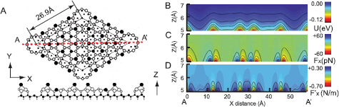
Figure 9. (A) Schematic figure of Si(1 1 1) . (B) Potential energy, as calculated with a Morse interaction between tip and adatoms. (C) Lateral forces, derived from (B). (D) Lateral force gradient, as derived from (C). Reprinted figure with permission from [44], Copyright (2009) by the American Physical Society.
Download figure:
Standard image High-resolution imageIn 2005, Kawai, Kitamura, Kobayashi and Kawakatsu again investigated the Si(1 1 1) surface, this time with a setup similar to Pfeiffer and co-workers, and an amplitude of 1 nm [43]. They made several interesting observations. The first was a spectrum of the torsional frequency shift
  as a function of the tip-sample height. Interestingly, the shape of the curve is similar to that expected from a normal FM-AFM z spectrum. This could be from a misalignment of the tip oscillation with the surface, similar to that discussed by Giessibl and co-workers. They then image their surface with a constant
  Hz. Although they are able to achieve atomic resolution, they observe only nine adatoms in the unit cell. The authors propose that this is because of the lateral oscillation, and that three pairs of adatoms appear merged with oneanother.
3.2. Smaller amplitudes and the role of STM feedback
In 2009, Atabak, Ünverdi, Özer and Oral described driving a vertically-mounted cantilever (such that the tip would oscillate along the surface, as proposed by Giessibl and co-workers [32]) at a frequency much lower than the natural oscillation frequency of the cantilever [4]. The low response of a damped harmonic oscillator made it easier for them to drive the oscillation at sub-Angstrom amplitudes. They regulate the tip-sample distance with simultaneous STM, and measure the amplitude of the cantilever oscillation, from which they derive the lateral force gradient. Although the authors do not resolve the atomic lattice, they do oberve an increase in lateral stiffness across step edges. They also perform z spectroscopy, concluding that there are substantial lateral forces during typical STM experiments. Most importantly from this contribution is the realization of sub-Angstrom oscillations required for high spatial resolution.
Kawai, Kawakatsu and Sasaki re-visited the Si(1 1 1) surface with LFM measurements and sub-Angstrom amplitudes, this time 81 pm [44]. They calculate the potential energy as a function of x and z, assuming that the tip interaction with the silicon adatoms can be described with a Morse potential, shown in figure 9(B). A lateral derivative, shown in figure 9(C), yields the lateral force. Finally, a derivative of the lateral force yields the lateral force gradient, shown in figure 9(D). Note that, if one was to acquire a constant-height scan of the Si(1 1 1)
 at a height of 5 Å, the signal above a single adatom would be a rich mix of positive and negative frequency shifts. Unlike the method proposed by Atabak et al [4], Kawai and co-workers excite the torsional mode of the cantilever, similar to [43]. Kawai and co-workers measure with STM feedback, estimating their tip-sample distance to be between 5.9 and 6.6 Å, a distance in which the adatoms appear as positive frequency shifts, and the space between them as negative frequency shifts.
Sasaki, Kawai and Kawakatsu then model the effect of using STM feedback on nc-LFM measurements of Si(1 1 1) [70]. Especially when measuring with STM feedback over the Si(1 1 1)
 surface, the tip cannot be assumed to remain at a constant height over the surface. They simulate nc-LFM data as well as the corresponding STM image over a range of amplitudes, from 37 pm to 760 pm. The nc-LFM simulation is in good agreement with the experimental data, showing a rich variety of contrast depending on whether the amplitude is small relative to the interatomic spacing or not.
3.3. Graphite: vertically soft and laterally stiff
In 2010, Kawai, Glatzel, Koch, Such, Baratoff and Meyer reported on an investigation of graphite [42]. This is perhaps an ideal candidate for nc-LFM: it is a layered material which is vertically soft, and yet laterally very stiff. Kawai and co-workers note that, with respect to nc-AFM, 'stable imaging with atomic resolution has so far succeeded only at low temperature'.
The authors use a standard silicon cantilever and, in contrast to Kawai's previous two papers, excite both the normal bending mode as well as the torsional mode, sketched in figure 10(A). The advantage of this is to prevent the soft cantilever ( N
N  ) from pressing down against the surface. By exciting the bending mode with a relatively large amplitude (15 nm), the restoring force acting on the tip, when it is close to the surface, is large enough to prevent the tip from crashing even with relatively large attractive forces at play. The torsional mode has a higher spring constant (
 N
N  ) and can therefore be reliably excited at low ampltiudes. Here, the authors use a torsional amplitude
  pm, much smaller than the lattice spacing of 246 pm, and acquire atomic resolution of this challenging surface, shown in figures 10(B) and (C). Simultaneous excitation of the bending and torsional modes complicates data analysis slightly, however they simulate a typical measurement and show that the frequency shift of the torsional mode follows the lateral force gradient.
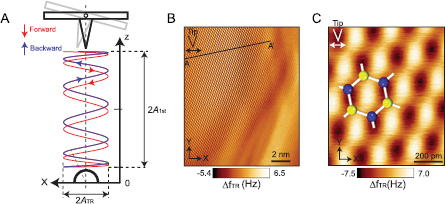
Figure 10. (A) Diagram of the bimodal mode used by Kawai and co-workers [42]. (B) nc-LFM image of HOPG with atomic resolution. (C) Zoom-in with lattice overlain. Reprinted figure with permission from [42], Copyright (2010) by the American Physical Society.
Download figure:
Standard image High-resolution image3.4. Friction anisotropy at the atomic scale
Since the work of Mate and co-workers, friction has been at the heart of many lateral measurements. Weymouth, Meuer, Mutombo, Wutscher, Ondracek, Jelinek and Giessibl took this problem and reduced it to its natural limit—a single atom—and showed that these forces are measurably different depending upon the direction [80].
The Si(1 0 0) surface reconstructs into rows of Si dimers that align on each atomic terrace, but are orthogonal to the rows on the terrace one step down, shown in figure 11(A). We exposed the surface with hydrogen so the dimers assume a symmetric configuration and are less reactive [11]. By aligning the sample such that the tip oscillation is parallel to the Si dimers on a given terrace, then by moving to the lower (or upper) terrace, the tip will oscillate perpendicular to the Si dimers. This allowed us to investigate the stiffness both parallel and perpendicular to the Si dimers, as shown in the nc-LFM image in figure 11(B). To collect data over two terraces, we used STM feedback. This brought up the same questions posed by Kawai and co-workers, opening the question of how much influence the tip motion due to the STM feedback has on the  data. We compared data collected with and without STM feedback: the contrast did not change significantly, and therefore the tip motion due to the STM feedback has a negligible influence on the
  data.
data.
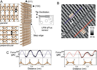
Figure 11. (A) Diagram of the qPlus sensor oriented for nc-LFM measurements. (B) nc-LFM image of H-terminated Si(1 0 0). The oscillation direction is shown in the white arrow. (C) Experimentally-determined force profiles (solid line) are in excellent agreement with the profiles calculated with DFT. Reprinted figure with permission from [80]. Copyright 2013 by the American Physical Society.
Download figure:
Standard image High-resolution imageIn motion perpendicular to the dimers, a maximum contrast of  N
N  is measured, whereas parallel to the Si dimers it is
  N
N  . In parallel, theoretical investigations were done with DFT-based simulations. Not only are the profiles in good agreement, but the magnitudes of the forces are also in excellent agreement, shown in figure 11(C). We are therefore able to successfully model wearless friction at the atomic scale with a realistic model. Furthermore, crystallographic and dimer alignment does play a measurable role on the well-defined Si(1 0 0) surface with respect to frictional forces.
Very recently, Naitoh, Turanský, Brndiar, Li, Štich and Sugawara investigated a similar system, the unsaturated Ge(0 0 1) surface, with a combination of bimodal FM-AFM and DFT-based simulations [62]. Like the work of Kawai and co-workers [42] the authors measure the frequency shifts of the cantilever both oscillating normal and parallel to the surface with the torsional mode. Similar to our work on Si(1 0 0) [80], the authors collect data over both high-symmetry directions by moving from one terrace to the next. As they record lateral and normal forces simultaneously, they are therefore able to produce a full three-dimensional map of the force vectors above a Ge dimer.
Similar to unsaturated Si(1 0 0), the unsaturated Ge(0 0 1) surface consists of dimers that are asymmetric. The authors note that at closer tip-sample distances, the two atoms of the dimer appear to have mirror-symmetry. With help of the DFT simulations, they propose that the tip induces this symmetrization.
3.5. Bending of a single molecule
Molecular deformation is difficult to measure, and yet has strong implications in chemical reactions. In the AFM community, this issue took a concrete shape a few years ago, when Gross and co-workers showed that the spatial resolution of atomic force microscopy can be drastically increased by terminating the tip with a single carbon monoxide (CO) molecule [34]. Although a CO-terminated tip apex was able to resolve the internal structure of molecules, it is not stiff, and lateral forces distort images (e.g. [63]). In order to interpret AFM data, a quantitative understanding of the CO tip was required. Specifically, we made the assumption that the CO molecule acts as a torsional spring, and set out to determine the torsional spring constant.
We used a CO-terminated tip to probe a single CO molecule on Cu(1 1 1) [79]. The experimental results were collected both with a normal-force FM-AFM and with a LFM setup. The data acquired with a normal AFM sensor showed the binding energy between the two molecules to be 8.4 meV.
We then used a lateral force sensor, also with a CO-terminated tip, to probe a surface CO molecule, measuring the lateral forces as a function of both lateral and vertical position, shown in figure 12(A). A torsional spring will bend at all positions except where the lateral forces are zero, correlating to positions where the potential energy is minimized. These positions, shown in figure 12(A) as black points, lie on a circle whose radius, 385 pm, is the equilibrium distance between the oxygen atoms.

Figure 12. (A) Model of the CO-terminated tip and the surface CO molecule, with lateral forces. (B) nc-LFM image of a CO molecule taken with a CO-terminated tip. (C) Calculated image. (D) Line scans of the data and calculated image, showing excellent agreement. From [79]. Reprinted with permission from AAAS.
Download figure:
Standard image High-resolution image
By assuming that both molecules act as torsional springs, and that the spring constant of the CO on the surface is known, we used the LFM data to determine the spring constant of the CO molecule on the tip. The best fit yielded a value of  zNm. Data and model output at all measured tip-sample distances show excellent agreement, such as those shown in figures 12(B) to (D).
4. Conclusion and outlook
From the initial work of Mate and co-workers, research into the techniques and applications of lateral force microscopy has blossomed. Soft cantilevers can be used in the lateral configuration because they are vertically stiff, and no longer suffer from jump-to-contact. nc-LFM was used to investigate non-contact friction, showing the clear influence of the electronic structure of the surface on the friction coefficient. It was also sensitive enough to detect the flipping of a single spin.
High spatial resolution requires amplitudes of oscillation smaller than the feature of interest on the surface. Atomic resolution therefore typically requires sub-Angstrom amplitudes of oscillation, and a cantilever stiff enough such that surface interaction will be a small perturbation of the tip oscillation. This is achieved by using either the stiff torsional mode of a standard cantilever, or a stiff cantilever like the qPlus sensor oscillating along the surface.
In order to explicitly measure potential energy, normal nc-AFM measurements must subtract the effects of long-range interactions, either by estimating the long-range component or by measuring it away from an adsorbate of interest. No longer sensitive to the large long-range van der Waals and electrostatic interactions, LFM measurements are ideal for the detection of short-range interactions.
Acknowledgments
Many thanks to Franz J Giessibl for his enthusiasm in force microscopy, in that he is always willing to help explore a problem with me, no matter how trivial or complex. I have had the pleasure of working with many people in the field of LFM including T Wutscher, D Meuer, and more recently, S Matencio and E Riegel. My thanks also to F Huber and S Matencio for their proofreading of the manuscript. Finally, I acknowledge support from the Deutsche Forschungsgemeinschaft (Grant No. GRK 1570).