
Abstract
Experimentally monitoring the dynamics of a physical system, one cannot possibly resolve all the microstates or all the transitions between them. Theoretically, these partially observed systems are modeled by considering only the observed states and transitions while the rest are hidden, by merging microstates into a single mesostate, or by decimating unobserved states. The deviation of a system from thermal equilibrium can be characterized by a non-zero value of the entropy production rate (EPR). Based on the partially observed information of the states or transitions, one can only infer a lower bound on the total EPR. Previous studies focused on several approaches to optimize the lower bounds on the EPR, fluctuation theorems associated with the apparent EPR, information regarding the network topology inferred from partial information, etc. Here, we calculate partial EPR values of Markov chains driven by external forces from different notions of partial information. We calculate partial EPR from state-based coarse-graining, namely decimation and two lumping protocols with different constraints, either preserving transition flux, or the occupancy number correlation function. Finally, we compare these partial EPR values with the EPR inferred from the observed cycle affinity. Our results can further be extended to other networks and various external driving forces.
Export citation and abstract BibTeX RIS
1. Introduction
Entropy production (EP) is a thermodynamic quantity intimately tied to the irreversibility of a nonequilibrium process [1, 2]. The EP sets fundamental bounds on the efficiency of physical systems like heat engines [2] and biological processes [3–6], and provides insight into the thermodynamics of nonequilibrium systems [7]. Estimating the total EP along a trajectory requires access to the entropy change of the system and the amount of heat dissipated to the surrounding reservoirs during the process [2, 8]. A major challenge in EP inference is the large number of out-of-equilibrium degrees of freedom, many of which are not accessible to an external observer and cannot be directly resolved [9, 10]. Nevertheless, a lower bound on the total EP can be obtained, for example, based on the fluctuations of an observed thermodynamic flux, like transition currents [11–14] or first passage times of the current [15–17], by the thermodynamic uncertainty relations. In essence, one can only estimate a lower bound on the total EP for a partially observed system. The observations can be, due to the finite spatiotemporal resolution, a subset of the 'states' [18–23] or a subset of the 'transitions' [24, 25] between the different states.
Theoretically, the effective, coarse-grained dynamics of various chemical and biological processes which occur over a wide range of timescales can be written in terms of the slow timescale processes while taking into account the action of the fast ones [26, 27]. A coarse-grained system, however, might appear to be time-reversible despite underlying nonequilibrium dynamics in hidden cycles [26, 27]. Still, eliminating fast degrees of freedom does not necessarily alter the apparent EP if the cycle carrying the probability current is not removed in the decimation process [28]. Coarse-graining of this kind was first studied using a Markovian master equation, and the coarse-grained EP was shown to satisfy a Fluctuation theorem [29]. In other scenarios, the entropy production rate (EPR) estimation for a coarse-grained system can exactly produce the total EPR. For example, by decimating states [30] while considering the inclusion of self-loops, the EPR obtained from a Markovianized master equation for the underlying non-Markov process estimates the actual EPR. Moreover, proper coarse-graining in the cycle space [31], or reducing bridge-states [32], can also preserve the mean EPR. Finally, observing a single transition in a unicycle network is sufficient to recover the total EPR [18, 24, 25].
EPR estimators for partially accessible systems have been studied widely, and several approaches have been proposed, including the passive partial entropy production (PPEP) and informed partial entropy production (IPEP) [18–23, 33], which provide a lower bound on the total EPR. For the case of the PPEP estimation, the observer has access only to a few microstates and the transitions between them. In contrast, in the IPEP estimation, the observer relies on the observed dynamics and the affinity of the observed cycles. Both the PPEP and the IPEP fail at stalling conditions, e.g. in the absence of a net current along the accessible link. However, the Kullback-Leibler divergence (KLD) estimator based on the asymmetry of the waiting time distributions (WTDs) can provide a tighter lower bound in the absence of the net flux along the observed link for second-order Markov processes [19, 24, 34, 35]. Recently, EPR estimators have been proposed based on observed transitions rather than observed states [24, 25]. The lower bound on the total EPR was estimated based on observing two successive repeated transitions along the same direction and the waiting times between the transitions or the 'inter-transition time' [24, 25]. The topology information of the network can also be deduced using this method from a single observed link for a unicyclic network or multiple observed links for a general Markov network [25]. The transition-based estimators equal the informed partial EPR for a unicyclic network [18, 25] and a general Markov network without hidden cycles.
Several attempts have been made to find a tighter bound on the total EPR. One approach suggests fitting the observed dynamics of a discrete-time Markov chain to an underlying Markov model that produces the observed statistics of the coarse-grained system [36]. When the number of hidden states is known, this fitting method can provide a tight bound on the total EPR. Moreover, two recently developed estimators are based on an optimization process of searching over possible underlying Markov models that obey the observed statistics of mass transfer between the mesostates [37] and the WTDs for the time forward and time-reversed transitions [38]. A novel approach for utilizing waiting time information by reformulation of the observed statistics of intra-transitions within macrostates was demonstrated to yield an improved lower bound on the EPR [39]. Further, a hierarchy of EPR estimators has been recently proposed, by optimizing over systems with the same observed mass rates and the same moments of the WTDs between coarse-grained states [40].
In general, there are two notions of partial information. In the first notion, the observer can distinguish between the observed and the hidden part of the system, where no information about the network topology is available for the hidden subsystem. Here, the sum of the partial EP of the observed and the hidden subsystems equals the total EP [18]. The other notion involves coarse-graining [28, 29, 32, 41–48], performed by lumping, i.e. merging several states into a single compound state [49, 50], or decimating [30] states. In decimation, the probability densities of the decimated states equal zero and are redistributed between the probability densities of the surviving states [51]. Similarly, in lumping [49, 50], the steady-state probabilities of the merged states sum up, whereas the rest of the states are not affected. In addition, one lumping protocol preserves the transition fluxes between the states, except for the states undergoing lumping [49]. However, another specific procedure for lumping conserves the time-dependent occupation number correlation function after the coarse-graining [50]. The accountability of the internal dissipation of the state undergoing coarse-graining is not guaranteed and depends on the coarse-graining procedure. Generally, coarse-graining is one method by which partially observed systems are often modeled. Further details on the different coarse-graining methods are discussed in the upcoming sections.
Here, we study how the above notions of partial information affect the partial EPR values obtained from partially observed systems. We start with the evolution equation for the EP of a driven system governed by a Master Equation, introduce lumping and decimation procedures on the system states, and obtain the partial EPR from an approximated Master (AM) equation. We further compare EPR values obtained from different coarse-graining approaches for different network topologies with the total mean EPR values.
The paper is organized as follows. First, we briefly review the EPR obtained from partially observed systems with observed and hidden substates in section 2. Next, we discuss the EPR inferred following the various coarse-graining methods. Section 3 shows the calculation of the total mean EPR from the evolution of the EP for a Markov chain and the evaluation of the partial mean EPR from the non-Markovian coarse-grained system following AM equation. Section 4 discusses the decimation method and the mean EPRs (scaled cumulant generating function (SCGF) and AM) obtained from their respective AM equations. In section 5, we describe two different lumping coarse-graining methods and calculate the corresponding mean EPRs. We discuss our results in section 6, and, finally, conclude our findings in section 7.
1.1. Partial EPRs
We consider a continuous-time Markov chain over a finite number of discrete states. The generator of the Markov jump-process, or the transition rate matrix, is defined by a matrix  . The non-diagonal elements (
![${w_{ji}} = {\left[ {\boldsymbol{{W}}} \right]_{j \ne i}}$](https://content.cld.iop.org/journals/0022-3727/56/25/254001/revision2/dacc957ieqn23.gif) ) of the matrix refer to transition rates between different states i and j, where
) of the matrix refer to transition rates between different states i and j, where  is non-zero only if
  is non-zero. The diagonal elements (
![${w_{ii}} = {\left[ {\boldsymbol{{W}}} \right]_{i = j}}$](https://content.cld.iop.org/journals/0022-3727/56/25/254001/revision2/dacc957ieqn26.gif) ) represent exit rates (
) represent exit rates ( ) from a particular state i. The evolution of the state probabilities is governed by a Master Equation
 , where
  denotes the time derivative, and
  denotes the probability vector to find the system in the respective states at time t. The system reaches a steady state at the long-time limit, denoted by the state probabilities vector
  , which can be obtained from solving
  . The distributions at steady state can also be obtained directly from the transition rates using the matrix-tree theorem [23, 52]. The stationary current between states i and j is defined by
  .
.
We start with simple yet non-trivial networks of continuous-time Markov chains (figure 1) [18, 53] to calculate the mean partial EPR for partially observed dynamics. In our model, we chose a system with 4 microstates, in which states 1 and 2 are observed, whereas states 3 and 4 cannot be distinguished, and are masked into a coarse-grained hidden state, H, as shown in the shaded area of figure 1. In practical scenarios, one can only observe a few transitions among states, and only a subset of the states. In PPEP, the observer only has access to an observed link between two microstates and the transition rates  between them
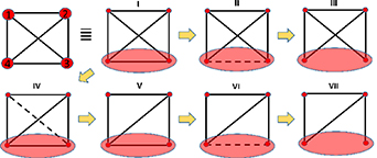
Figure 1. Different network topologies in which states 1 and 2 are observed, and states 3 and 4 are indistinguishable, and collectively called 'hidden state' (shaded with red color). The weights of the 3–4 link and 1–3 link are denoted by  and
and  , respectively. The networks are denoted by these two parameters (I)
  (II)
(II)  (III)
(III)  (IV)
(IV) (V)
(V)  (VI)
(VI)  (VII)
(VII)  . The other transition rates are:
  ,
, ,
,  ,
,  ,
,  ,
,  ,
,  ,
,  ,
,  ,
,  ,
,  ,
,  .
.
Download figure:
Standard image High-resolution imageAt a long time limit, the PPEP reaches its steady-state rate [18, 21–23], given by

where  is the natural logarithm in base e.
On the other hand, for the IPEP [18, 21–23], in addition to the cycle affinity of the observed link, one has access to the steady state probability densities of both of the observed states at stalling conditions. For calculating the IPEP, we additionally assume that the observer can tune the rates over the observed link and use the system's steady state probabilities when the new rates are applied to infer information about the hidden states. The observer can tune the transition rates according to  and, with driving force
  of dimension
 and
and  dimensionless.
  is the characteristic length scale, and
  is the inverse temperature. To calculate the IPEP, the system is tuned to stalling conditions, in which the current over the observed link vanishes at
  , and the resulting steady-state probability densities of the two observed states are
  , and
, and  , respectively. At a long-time limit, the IPEP rate is given by [18, 23]:

The stalling distribution can be calculated by solving  , where the modified generator
  is obtained by setting the rates over the observed link (1–2 link) as zero in the original Markov rate matrix
  , i.e.
  = 0 and adjusting the exit rates accordingly (see [18, 21–23] for full derivation). The value of the stalling force can then be calculated according to
  .
.
Due to added information about the hidden states through the stall force, IPEP provides a better bound to the total EPR compared to the PPEP [18], and therefore we only compare to IPEP in the following. In this manuscript, we assume to have access only to the state information, without having knowledge regarding the fluctuations of the thermodynamic flux, first passage time associated with the thermodynamic flux, and waiting time information.
1.2. EPR estimation from master equation
We consider a trajectory  with a sequence of N states
  and the corresponding waiting times
  for a total observation time
  ,
,  , given by
  . The probability of observing such a trajectory is given by

Similarly, one can define the probability ![$\tilde P\left[ {\tilde \gamma } \right]$](https://content.cld.iop.org/journals/0022-3727/56/25/254001/revision2/dacc957ieqn56.gif) for the time-reversed trajectory
for the time-reversed trajectory  , and express the total EP along the trajectory,
  using their ratio [18]:
where  is the net number of transitions from state
  to state
  .
.
The EPR can be calculated from the evolution of the EP governed by the Master equation. Following Teza and Stella [30], we denote the probability  that the system is at state i at time t, and have produced entropy
  from all possible trajectories up to that time. Since each transition between a pair of states i and j adds up
  to the total EP, we can write Master Equations for all the state probabilities
  having EP S at time t:

where  is the exit or the escape rate from a particular state i. Let us denote
 , where
  is the discrete Laplace transform of
  with respect to the entropy S. We reformulate equation (5) as:
Equation (6) can be cast in matrix form as , with
  being a column vector with
  as its
  th entry, and
  the tilted transition matrix [30, 54]:
The dominant eigenvalue ( of the tilted transition matrix,
  , is the SCGF of the EP. The mean EPR can be calculated from [30, 54, 55]:

TM refers to 'Total mean' (figure 2) as all the states' dynamics have been considered during its calculation.
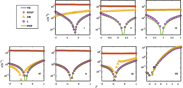
Figure 2. Mean EPR estimation from the total mean (TM) or  , scaled cumulant generating function (SCGF or
  ), from approximated master equation (AM or
  ), lumping by preserving the transition flux and steady-state probabilities (L or
  ), informed partial entropy production (IPEP or
  ) for different network topologies. The parameter values for each subplot (network topology, I–VII) are the same as mentioned in figure 1. The ranges of the x-axes were chosen to include the stall force and to show the behavior of the estimators around and away from it.
Download figure:
Standard image High-resolution imageIn the next sections, we discuss EP obtained from the decimation and the lumping coarse-graining methods. In each of the methods, we find a Markovianized rate matrix ( associated with the coarse-grained system dynamics, modelled by an AM equation of the form
  , where
  is the column vector of probability densities of the coarse-grained states at time t.
1.3. Coarse graining via decimation
Decimation involves removing some states and redistributing their population density among the rest of the states. In this section, we consider decimating one of the states, say state d from equation (5), and evaluate the mean EPR from the decimated system. To do so, we perform the following four steps [30, 51].
We start with the following Master equation in terms of the probability of the EP:
where  is the exit rate from state i,
  is the transition rates between different states
  and
and  , and
, and  is the probability of being in state
  and having EP
  at time
  .
.
The terms are the same as mentioned in section 3. First, we Fourier transform equation (9) using  , where i includes all the states. Second, we substitute
  in the Fourier transformed equations, where
  is given by
Substituting  in the Fourier transformed equations, we obtain the following:
Multiplying both sides by ( , we get
Third, we perform the inverse Fourier transform on  , and we obtain second-order differential equations. However, we only retain the first-order terms in t, i.e.
  (t) therefore considering a Markovianized approximation [51]. In order to get the same mean EPR as the mean total EPR (TM) after coarse-graining at steady-state, we use an approximation following [51] for the proportionality relation between states i and j at steady state
After the decimation of state d (i.e. redistributing  among other states), the remaining states have renormalized probabilities that sum up to 1. If state d is decimated, then the probability of being in the decimated state d in the coarse-grained system equals zero,
  However, the occupation probabilities of the rest of the states
  are affected by the transition probability
  from the decimated state d to state i in order to preserve the population density. Thus, in the fourth and the last step, the probabilities are renormalized according to
  where
where  is the probability of the coarse-grained state i,
  is the probability before the coarse-graining, and
  is the transition probability from state d to state i. The transition probability is given by the ratio of the transition rate from state d to state i (
 to the total exit rate from state d (
 , i.e.
  .
.
Using  as an approximation [51], and consider this relation to hold throughout the evolution, we find the relation between the probabilities of a state before and after the decimation. From,
  we get
where  , and
, and  .
.
The equation in terms of the probability distribution function for the EP of the coarse-grained state is written by
where  and
and  .
.
We now write the equations for the transformed variable associated with the coarse-grained states, , as follows:
We want to emphasize that  is also a function of the transition rates
 , but for the sake of simplicity, we show the explicit dependencies only on
  and t. In matrix notation, equation (15) can be written as

with the matrix elements of  being
being
We calculate the mean EPR from the scaled cumulant generating function,  , which is the dominant eigenvalue of the
  tilted transition matrix
  The mean EPR (
 is calculated in the following way

We refer to this mean EPR as SCGF (figure 2) as this quantity is calculated from the scaled cumulant generating function of the EP.
As mentioned earlier at the end of section 3, we consider the coarse-grained system dynamics to follow an AM equation with effective transition rates, derived from equation (14). We write the approximated equation governed by the probability density of the coarse-grained system to be in the coarse-grained state  (where
  ) at time t as the following,
In terms of the probability distribution of the EP,  , we obtain similar equation as equation (14), which we can rewrite in terms of the generating function,
  ,
,
In matrix notation which reads as  , where AM stands for EP obtained from the AM equation. As previously, a tilted matrix,
  , is used to calculate the mean EPR
We obtain the mean EPR from the dominant eigenvalue of the above matrix,  :
:

The mean EPR calculated using this value is shown as AM in figure 2.
1.4. Coarse graining via lumping
A different strategy of coarse-graining is lumping several microstates into a single mesostate  . Our goal is to find a rate matrix by the lumping method [49] where the coarse-grained system dynamics follow an AM equation. The probabilities of the merged states,
  , are summed up, while the steady states probabilities of the rest of the states remain unchanged,
In this scenario, the coarse-grained transition rates are modified to conserve the steady-state probabilities and the transition flux among all the states except for the flux between the merged states, so the coarse-grained system is expected to have similar steady-state properties as the original system [49]. As the affinity is not preserved in this method, the EPR of the coarse-grained system is changed. The modified rates for the AM equation are as follows [49]:
These transition rates are proven to minimize the KLD of the trajectories and can be used for lumping any two states even without a timescale separation [49]. The diagonal terms of the coarse-grained transition matrix are  . We calculate the mean EPR from the following tilted transition matrix
The mean EPR is obtained from the dominant eigenvalue of the matrix, 

where the mean EPR from this matrix is referred to in figure 2 as L (lumping with preserving steady-state properties).
Hummer and Szabo [50] developed another procedure for defining a transition rate matrix for a coarse-grained system. Their method ensures that the time-dependent occupancy number correlation functions in the coarse-grained system are equal to the ones of the original system. The same reduced matrix (rate matrix for the coarse-grained system) can be obtained from the projection operator technique. In the approximated Markovian limit, the reduced transition rate matrix was calculated analytically [50]. This coarse-graining procedure of merging or lumping microstates into a single merged state was suggested to be used for optimal aggregation and applied to Markov chains, random walk models, models with discrete states and discrete time, and with continuous states and discrete time. This coarse-graining method works well at intermediate timescale. The autocorrelation function between coarse-grained states I and J at time t is defined by  , where
  equals 1 when the system is at state I. The autocorrelation function of the coarse-grained system and the full system are related by
  . At the Markovian limit, the reduced matrix
  is given by [50]:

where the initial rate matrix  is of order n-by-n (being the number of microstates), and the reduced matrix
  is of the order of N-by-N (
 is the number of coarse-grained states after merging). The normalized equilibrium probability density for the merged state
  is given by
  , and the matrix obeys
  , where
  is a column vector with entries
  . The elements with the suffix N (n) refer to the merged states (constituent microstates).
  and
and  are the diagonal matrices with the equilibrium distributions as diagonal elements.
  is the unit matrix of dimension N-by-N.
A
is the adjacency matrix of dimension n-by-N, defined as
is the unit matrix of dimension N-by-N.
A
is the adjacency matrix of dimension n-by-N, defined as  for
for  I. The adjacency matrix (
A
) was introduced to map the coarse-grained system onto the full system via matrix notation. Note that the expression in equation (27) for the coarse-grained system is a reduced form of the full system transition rate matrix
I. The adjacency matrix (
A
) was introduced to map the coarse-grained system onto the full system via matrix notation. Note that the expression in equation (27) for the coarse-grained system is a reduced form of the full system transition rate matrix  The reduced matrix can have negative off-diagonal elements [50], and therefore, it is not a 'true' transition rate matrix. We calculate the mean EPR from the tilted transition matrix
  , and call it HS.
where ![${\left[ {\boldsymbol{{R}}} \right]_{ji}}$](https://content.cld.iop.org/journals/0022-3727/56/25/254001/revision2/dacc957ieqn152.gif) is the
is the  element of the transition matrix
  . HS is calculated from the dominant eigenvalue of the matrix,

We compare the mean EPR values obtained from the lumping and decimation coarse-graining methods, with the informed partial EP for the networks shown in figure 2. The results are presented and discussed in the next section.
2. Results and discussion
In this section, we compare EPR obtained from different methods like SCGF, AM (AM equation), L (coarse-graining method where the transition flux among all states except the merged states and the steady state probabilities are preserved), IPEP (considering parameter dependent transition rates between the observed states), HS (considering the time dependent occupation number correlation function to be preserved) with TM (true mean value of the EPR considering all the edges). The closer the mean EPR values predicted from different coarse-graining methods to the TM, the better is the prediction. In all the methods mentioned above, we consider the coarse-grained system dynamics to follow AM equations. Therefore, the error of the approximation is expected to be smaller if there is a timescale separation (except for the lumping). Except for SCGF, all other state-based coarse-graining methods (AM, L, HS) are calculated from tilted matrices based on the corresponding modified rate matrices, given by equations (21), (25), and (27), respectively. We calculate the mean EPRs from different state-based coarse-graining methods like lumping and decimation and compare them with the mean EPR obtained from partial information of only the observed link, i.e. IPEP (equation (2)). For partially observed systems, we always get lower bounds on the total EPR. Therefore, the higher the bound, the better it is, as it provides a tighter estimation of the total EPR.
We plot TM, SCGF, AM, L, and IPEP as a function of dimensionless driving forces ( ) for different network topologies, as shown in figure 1. All the parameter values are given in the caption of figure 1, and the subplots of figure 2 correspond to the same network topologies as in figure 1.
In figure 2, we present TM, SCGF, AM, L, and IPEP correspond to  ,
,  ,
,  ,
,  , and
, and  as calculated using equations (8), (18), (22), (26), and (2), respectively. TM provides the mean EPR for fully observed systems, so the closer the EPR bounds to the TM, the better the estimators. The mean EPR obtained from the scaled cumulant generating function of the EP (
 or SCGF) by decimating one of the states (applying all the constraints mentioned before equation (13)) always estimates the total mean EPR (
 or TM), as expected. In other words, the decimation procedure is constructed in a manner that it reproduces the mean EPR at steady states. As the EPR's are calculated at the steady state, the EPR from the scaled cumulant generating function exactly produces the TM. In the following, we compare the AM, L, HS, and IPEP with the total mean EPR values (TM) for all the network topologies.
The EPR calculated from the AM Equation ( or AM) provides a lower bound on the total mean EPR (
 or TM), since after decimation, the coarse-grained system is not Markovian, and therefore, the AM cannot capture the total EP. When the hidden substates are disconnected (network topology III and VII in figure 1), we do not lose any cycles carrying transition currents in the coarse-graining, so the AM provides values closer to the total mean EPR (
 . We note that for topology VII (figure 1), the observed information is sufficient for precisely inferring the total EP, since the observed cycle is the only entropy-producing fundamental cycle in the network, and the AM equals the total EPR (TM). In that case, the IPEP also equals the total EPR, as expected [18].
We further compare the mean EPR from a state-based coarse-graining (L), i.e. lumping by conserving the steady-state probabilities and the transition fluxes between all states except the merged states, with the IPEP. Since it is difficult to compare based on the subplots in figure 2, we plot  in figure 3, as a function of the driving force
  in semi-log plots. From figure 3(a), we find the difference between L and IPEP is larger for network topology III compared to I, near their corresponding stall forces (labeled with dash-dotted lines). For network topology V (figure 3(b)), with connected hidden states, the difference between
  and
and  is less than 0.1% for the range of
  values tested around the stall force, whereas for network topology VII, with disconnected hidden states, the difference
  is approximately two orders of magnitude larger compared to topology V, near the corresponding stall force. IPEP accounts for the hidden states transition information via a single rate, which is missing if the hidden states are disconnected, and therefore, the difference between the L and IPEP increases.
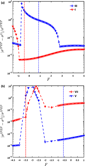
Figure 3. Comparison of  and
and  as a function of the dimensionless driving force
  for different network topologies: weight of the connectivity of the hidden substates and in between state 1 and state 3 are given by
  and
and  , respectively. The parameters used have the same values as mentioned in figure 1. (a) Red downward triangles and blue diamonds refer to network topology I and III, respectively. (b) Blue downward triangles and red diamonds refer to network topologies V and VII, respectively. The lines are drawn to guide the eye. The stalling forces are labeled by dash-dotted lines for each topology.
Download figure:
Standard image High-resolution imageIPEP is calculated from the observed cycle affinity, whereas L is based on preserving the steady state properties of the system, e.g. the probabilities and the transition fluxes. So, it is difficult to compare the trade-offs between the input information provided and its output (mean EPR estimation). We find that for connected hidden substates (network topology I and V), the difference between L and IPEP is smaller compared to disconnected hidden substates (network topology III and VII) at their respective stall forces.
In figure 4, we compare the EPR obtained from the two lumping methods described in section 5, namely, L, where the steady-state probabilities and the transition flux between the observed states are preserved, and HS where the autocorrelation function of the population for the coarse-grained states is the same as the full system. Both methods consider the coarse-grained system to follow approximated Markovian dynamics, and therefore, the error in the approximation varies depending on the timescale separation. The coarse-grained transition rates in equation (24) are based on minimizing the KLD between the trajectories, whereas the reduced matrix in equation (25) is constructed to maximize the relaxation time of the reduced matrix so that the coarse-grained system would have the same characteristic time as the full system. For both network topologies I (figure 4(a)) and V (figure 4(b)), L dominates over HS for certain driving parameter values (F), whereas for other driving parameter values, HS dominates over L. At stalling force, HS results in larger EPR values compared to L. The non-diagonal elements of the reduced matrix of topology I (equation (27)) become negative above a certain driving force (
 [50], and therefore we are unable to calculate HS beyond this value (figure 4(a)). As the HS coarse-graining approximation's accuracy depends on the timescale separation between the states undergoing merging and in between the merged states, EPR prediction using this coarse-graining method also depends on the intrinsic timescale difference. However, the method predicting L can be used without a timescale separation. Therefore, the performance of the estimators for the two coarse-graining approaches depends on the system at hand. The optimal Markov matrix, R (equation (27)), was calculated based on the assumption that there are no disconnected microstates, according to HS [50]. Therefore, we only compare the results among the two lumping methods for network topology I (figure 4(a)) and topology V (figure 4(b)) of figure 1.

Figure 4. Comparison between two lumping methods (L and HS) for (a) network topology I and (b) network topology V. The parameter values are the same as given in figure 1. The red downward triangles denote the HS method, and the purple circles refer to the L method. The stalling forces are labeled with dashed-dotted (a) red line for topology I, and (b) blue line for topology V.
Download figure:
Standard image High-resolution image
3. Conclusion
This paper studies different notions of partial information in driven systems and the corresponding mean EPR values associated with them. The predicted EPR values are then compared with the true mean EPR (TM) which is calculated considering all the edges of the network topology, where tighter lower bounds on the TM EPR are considered better. The SCGF, which is calculated for coarse-graining by decimation and redistribution of the steady-state probabilities and transition rates, produces the total mean EPR (TM), as expected. For the other coarse-graining approaches, systems are considered to follow approximated Markovian dynamics, and the resulting modified/coarse-grained transition rate matrices are used to calculate the mean EPRs for different methods (AM, L, HS). For certain topologies, we find that as we decrease the hidden state connectivity, the AM approaches the total mean EPR (topologies I, II, and III) since the contribution to the EPR from the loss cycles carrying transition flux decreases. By comparing the mean EPR values calculated from the state-based coarse-graining methods, namely, lumping (L, HS) and coarse-graining by decimation (SCGF, AM), where one is assumed to know the network topology, with the mean EPR inferred from partial information of only the observed states and the transitions between them (IPEP), we find that the effect of the partial information reflected on the inferred EPR for state-based coarse-graining depends on the network topology. Further, IPEP provides similar entropic information as one would obtain by L, a state-based coarse-graining (lumping with preserving the steady-state properties), where the difference between is bigger for disconnected hidden substates (topologies III and VII), compared to the networks with connected hidden substates (topologies I and III) at their corresponding stall force. Hidden state information inferred by the IPEP is lost for disconnected hidden substates, and due to this missing information, the difference between L and IPEP increases with decreasing connectivity between the hidden substates. The difference between the HS and L varies as a function of the stalling force, and the timescale difference plays a role in it. HS is sensitive towards the timescale separation in between the merged states and between two merged states, whereas L does not depend on the timescale separation. Our study can be extended to larger systems with more than two hidden microstates, or having a hidden cycle current, etc.
Acknowledgments
G Bisker acknowledges the Zuckerman STEM Leadership Program, and the Tel Aviv University Center for AI and Data Science (TAD). A Ghosal acknowledges the support of the Pikovsky Valazzi scholarship. This work was supported by the ERC NanoNonEq 101039127, the Air Force Office of Scientific Research (AFOSR) under Award Number FA9550-20-1-0426, and by the Army Research Office (ARO) under Grant No. W911NF-21-1-0101. The views and conclusions contained in this document are those of the authors and should not be interpreted as representing the official policies, either expressed or implied, of the Army Research Office or the U.S. Government. A Ghosal acknowledges helpful discussion with Dr Gianluca Teza.
Data availability statement
All data that support the findings of this study are included within the article (and any supplementary files).