
Abstract
Antiferromagnets (AFs) have recently surged as a prominent material platform for next-generation spintronic devices. Here we focus on the dynamics of the domain walls in AFs in the presence of magnetoelasticity. Based on a macroscopic phenomenological model, we demonstrate that magnetoelasticity defines both the equilibrium magnetic structure and dynamical magnetic properties of easy-plane AFs in linear and nonlinear regimes. We employ our model to treat non-homogeneous magnetic textures, namely an AF in a multi-domain state. Calculations of the eigen-modes of collective spin excitations and of the domain walls themselves are reported, even considering different kinds of domains. We also compare the output of our model with experimental results, substantiating the empirical observation, and showing that domain walls majorly affect the optically driven ultrafast nonlinear spin dynamics. Our model and its potential developments can become a general platform to handle a wide set of key concepts and physical regimes pivotal for further bolstering the research area of spintronics.
Export citation and abstract BibTeX RIS

Original content from this work may be used under the terms of the Creative Commons Attribution 4.0 license. Any further distribution of this work must maintain attribution to the author(s) and the title of the work, journal citation and DOI.
1. Introduction
Within the broad research area of magnetism, antiferromagnets (AFs) play a peculiar role, since insulating AFs represent the overwhelming majority of magnetically ordered materials in nature, and can display a variety of different textures (collinear, non-collinear, domain walls, skyrmions). Beyond the research activity driven by fundamental questions (e.g. the nature of the quantum mechanical ground state, which is not an eigenstate of the Heisenberg Hamiltonian), a recent dramatic surge of interest in AFs was ignited by the perspective to employ them in spintronics [1–3]. Such devices would possess the potential to outperform a technology based on materials with a net magnetic moment in their ground state. The reasons lying behind this research effort are the robustness of AFs against electromagnetic noise, the possibility of high-density of storage in possible memory devices and, most importantly, the intrinsic higher frequency of spin waves, in comparison to ferro- and ferri-magnets. This last point makes AFs an attractive platform for memory devices able to write, store and read information on a timescale, which is orders of magnitude shorter than analogous devices relying on ferromagnets. Therefore, spin dynamics in AFs have been measured in a broad variety of different regimes, schemes and employing different stimuli. Transport measurements revealed spin currents induced by magnons [4, 5], the spin Seebeck effect [6, 7] and the modification of the domain configuration [8, 9]. However, electrical techniques require either metallic AFs, which are very rare systems, or a heavy-metal layer on top of the dielectric AF in order to both excite and detect spin dynamics in the AF. Consequently, Joule dissipations are not avoidable. Moreover, the dispersion of magnons in AFs exhibits frequencies entering even the tens-of-THz regime, implying timescales not accessible by transport methods. It is thus natural to consider stimuli of comparable duration and, in particular, femtosecond laser pulses, since they can be directly employed even in dielectric materials, without requiring a heavy metal layer. In this case, Joule-dissipations are automatically ruled out. The optical excitation has already successfully enabled the coherent resonant [10, 11] and non-resonant [12] generation and control of both low- [13] and high-energy magnons [14, 15], even in the absence of lattice-heating [16].
A fundamental challenge and intrinsic obstacle in antiferromagnetic spintronics is the impossibility of generating a single-domain state under conventional laboratory conditions. This problem has been tackled in a variety of ways: thermally treating some AFs increases the size of domains up to a range of the 100 µm order [17, 18]; applying a huge magnetic field of the order of 60 T, generated in a dedicated facility, generates a single-domain-state [19]. Although these approaches have been successful in the context of state-of-the-art experiments, they are not practical solutions and, in particular, they are not feasible from the perspective of devices. Evidence that domain walls in combination with magnetoelasticity significantly affect the magnetic transport [20] and the optically driven ultrafast spin dynamics [21] is reported; nevertheless, a cohesive and general theoretical framework addressing how magnetoelasticity affects the magnetic texture in steady and transient dynamical states of AFs is lacking. Here we bridge this gap in fundamental knowledge, by deriving a macroscopic phenomenological model in which the role of magnetoelasticity on the domain distributions and on the spin dynamics is addressed. In particular, we demonstrate that magnetoelasticity plays a crucial role in defining the energy landscape of the magnetic system and pinning the domain walls, even in the absence of defects. The spectrum of magnons and of the walls of an AF in a multi-domain state is calculated. We then discuss the hybridization of the modes and the interaction between magnons and the walls, both in a linear and nonlinear regime of spin dynamics. In particular, we reproduce the experimental evidence that different magnon modes can couple in a multi-domain AF, via a magnetoelastic nonlinear interaction with the domain walls. Our theory is rather general, since we discuss both kinds of domains in AFs. Moreover, the same framework can be employed for different materials and different regimes of spin dynamics.
This paper is organized as follows. In section 2 the role of magnetoelasticity in the equilibrium properties of an AF in multi-domain states is discussed. The results of our work are presented in this section and are then rigorously proved in the following sections. The modeling is then introduced in section 3, applying the general framework to the already known case of a single-domain state. Section 4 reports the results of the model for the multi-domain state, in particular in terms of both spectral properties (of magnons and domain walls) described in the linear regime. Section 5 describes nonlinear effects in the spin dynamics induced by the presence of magnetoelasticity and domain walls. Possible extensions of our model, in terms of different sample properties and dynamical regimes, are discussed in section 6. The conclusions of our work are reported in section 7.
2. Qualitative considerations
In this section, we introduce the magnetoelastic interactions in AFs, explaining how they affect both the equilibrium magnetic texture and dynamical properties. All the statements here reported are qualitative and will be rigorously demonstrated in the following sections of the paper. This section thus provides an accessible overview of the core focus and main results of our model.
The magnetoelastic coupling affects the magnetic properties of AFs in a variety of ways. It emerges as spontaneous striction, following the onset of the long-range ordering, and defines a gap in the magnon spectrum [22, 23]. Moreover, it is also responsible for the reorientation of the Néel vector under externally applied stresses. Here we focus our discussion on magnetoelastic effects in multi-domain easy-plane AFs, which represent a wide class of materials (for instance NiO, MnO,CoO, α-Fe2O3, FeBO3). The spontaneous (i.e. internal) strains are inhomogeneously distributed in the material and map the magnetic domain structure. Therefore, in the following, the words inhomogeneous and multi-domain are interchangeable, while similarly the term homogeneous is synonymous with single-domain.
We consider a physical framework in which the temporal period of the lowest acoustic lattice mode is much larger than the period of spin waves. In this case, possible variations of the spontaneous strains are too slow to follow the spin dynamics, and the inhomogeneous strain field can be considered as static on the relevant timescale. This approximation, which is called 'frozen lattice', is justified in the description of ultrafast magnetic phenomena.
In order to provide a qualitative picture of the main results, let us start with the example of a simple collinear easy-plane AF, whose magnetic structure includes only two domains (named '1' and '2'). The orientations of the Néel vector in the two domains are orthogonal to each other, i.e.  . In the absence of magnetoelastic coupling, the magnetic energy has two equivalent minima corresponding to the easy magnetic axes (say
  and
and  ) and two maxima corresponding to the hard magnetic axes (
 ). The number of easy and hard axes is defined by the structure of the material, here assumed to be tetragonal as in the relevant case of NiO. The domain structure would consist of four types of domains [24], separated by 90∘ walls, satisfying geodesic conditions. Smooth 180∘ domain walls would be unstable with respect to the configuration in which they are split into pairs of 90∘ walls separated by 90∘ domains. Within this model, the displacement of a domain wall would cost no energy and can be considered as an activationless nonlinear excitation [25–27].
Spontaneous strains significantly change this picture by coupling with the Néel vector. An additional magnetic anisotropy is introduced, and the degeneracy between the two easy magnetic axes is lifted. Moreover, if the spontaneous strains are inhomogeneous, they determine a space-dependent orientation of the magnetic easy axis. This is illustrated in figure 1 where the magnetic texture is represented by the direction of the arrows (the Néel vector), while the different colors represent regions with different spontaneous strains (colors), and thus different easy axes. In equilibrium, the centers of the magnetic and elastic domain wall coincide (figure 1(a)), though the elastic domain wall is much thinner.
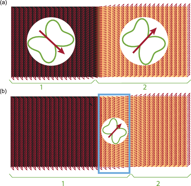
Figure 1. Profile of antiferromagnetic domain and domain walls pinned by spontaneous strains (color code). The arrows indicate the Néel vector. (a) Equilibrium configuration: the magnetic domains '1' and '2' coincide with the elastic domains (see discussion in the main text). The magnetoelasticity determines the easy axis of the Néel vector in the two domains, shown in the plots in polar coordinates. (b) Displaced magnetic domain wall (i.e. the sizes of '1' and '2' have changed) over a 'frozen strain' background, i.e. the color-coded elastic texture is unchanged. The magnetic energy of the framed region is higher compared to the energy in equilibrium configuration due to unfavorable orientation of the Néel vector.
Download figure:
Standard image High-resolution imageAn effect of inhomogeneous strains is the pinning of the magnetic domain wall. To illustrate this, let us consider a shift of the magnetic domain wall (figure 1(b)) with respect to the frozen elastic texture. This shift has an energy cost, since in the region between the equilibrium and the displaced positions of the domain wall center (marked with a box in figure 1(b)), the Néel vector deflects from the energetically favorable easy direction defined by a local strain. Such a displacement creates a restoring force, which can induce oscillations of the domain wall around the equilibrium position. Intuitively, the corresponding frequency should scale with the magnitude of the magnetoelastic parameter. The dynamics of the potential energy and magnetic anisotropy as the magnetoelastic parameter increases are shown in the supplementary movies (available online at stacks.iop.org/JPD/54/374004/mmedia).
Such an oscillating domain wall, with the Néel vector rotating in the easy plane, can also be interpreted as a localized nonlinear magnon mode with the same polarization as the in-plane magnon mode, which is shown in figure 2 (left panel). This consideration is important, since this is the reason why in-plane magnons propagating toward the wall can interact with it, being scattered and reflected. Differently, out-of-plane magnons (see figure 2, right panel) are transmitted without interaction with the domain boundary, because they are orthogonally polarized. We stress that the strain-induced pinning is the origin of both the domain wall oscillations and the wall-(in-plane)-magnon interaction described above. Another effect of magnetoelasticity is the stabilization of a 180∘ domain wall against the splitting into two 90∘ domain walls. This modification of the domain structure results from the discrimination and differentiation of the two easy directions ( and
and  ) introduced by the spontaneous strains.
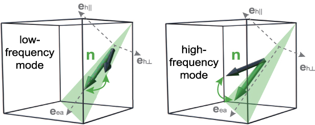
Figure 2. Polarizations of the eigen-modes in a single T-domain. The three unit vectors are shown. Left panel: in-plane mode, right panel: out-of-plane mode.
Download figure:
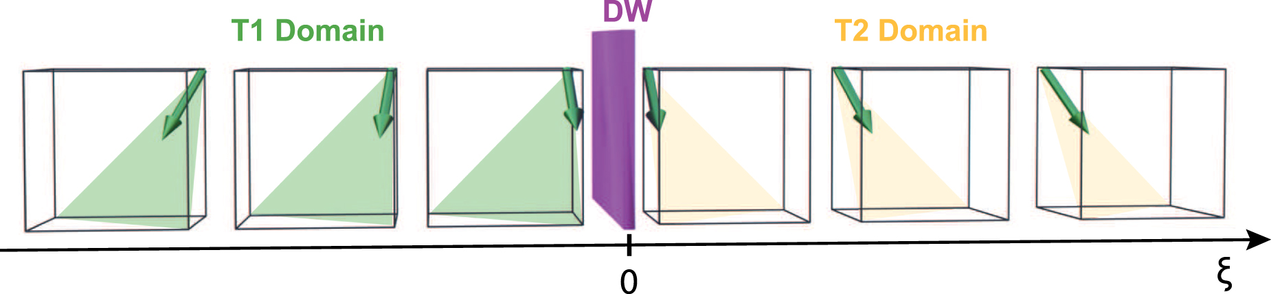
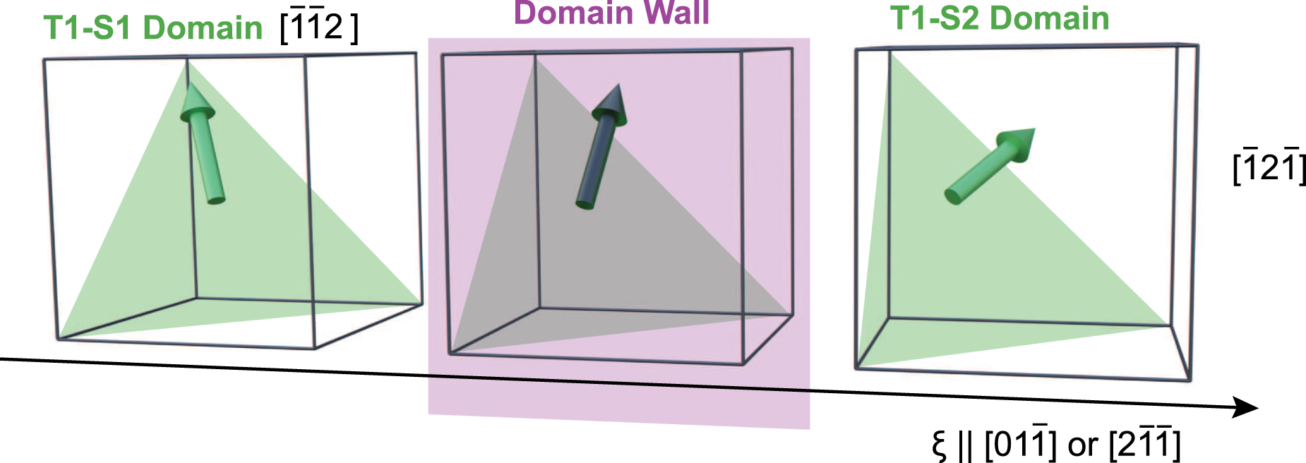
Standard image High-resolution imageGenerally, frozen strains can discriminate not only the easy axes of an AF, but also the orientation of the easy planes. This can happen in materials whose magnetic structure includes two types of domains: twin (T) and spin (S) domains. The latter are typical magnetic domains and can be found in most of the easy-plane AFs. The domains described above in this section are S-domains. T-domains, differently, are structural with different orientations of the crystallographic axes. In each T-domain, the orientation of the easy magnetic planes and even the definition of the Néel vector vary. Additionally, in the wall separating two different T-domains, the distribution of the Néel vector is not restricted to any of the easy-planes and is three-dimensional (see figure 3). However, as the antiferromagnetic vectors in different T-domains are coupled (due to the exchange interaction at the interfaces), the above considerations in this section apply to T-domains as well, though the distribution of the Néel vector in this case cannot be so easily represented graphically. Moreover, in this case, the strains pin the domain walls and even hybridize the magnon modes, enabling linear and nonlinear effects in the magnon dynamics. In the following sections, we consider these effects in more detail, using as a model the collinear easy-plane AF NiO. Our choice is motivated by the strong magnetoelastic coupling in NiO crystals, which is manifestly displayed in the equilibrium and transient magnetic properties of NiO. Moreover, this material has been extensively studied, also in terms of spintronic perspectives, being considered a prototypical Heisenberg AF. However, our model applies to the many other materials with similar structures, such as MnO, CoO [28], α-Fe2O3, FeBO3 and CuMnAs [29].
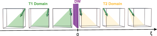
Figure 3. Domain wall between two T-domains in bulk NiO.
Download figure:
Standard image High-resolution image3. Model
In this section, we introduce the model and apply it to the homogeneous case, i.e. an AF in a single-domain state. According to the symmetry analysis, the magnetic structure of a single-domain NiO (type-II antiferromagnetic structure) [30–33] is described by one of the four Néel vectors  (j = 1–4), where the different wave vectors
  correspond to different T-domains (see table 1). In a multi-domain sample, the Néel vector
  coincides with an appropriate
  within each of the T-domains. Due to the exchange coupling between the Néel vectors with different
  at the boundary between the T-domains, we can consider the function
  as a continuous field variable in the whole sample (see appendix

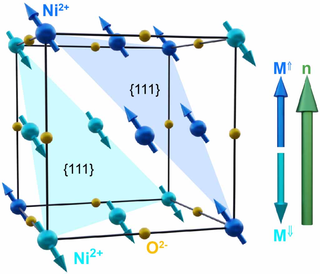
Figure 4. Crystallographic and magnetic structure of NiO. The two Ni2 + sublattices (M ) and the definition of the Néel vector (
 ≡ M
≡ M − M
− M ) are shown.
Download figure:
Standard image High-resolution imageTable 1. Classification of T- and S-domains and corresponding vectors of the local coordinate frame. The unit vector  is parallel to the magnetic easy axis and specifies that the-S domain,
  (
( ) is parallel to the hard magnetic axis in (out of) the easy plane.
| N | Domain |

|

|

| T plane |
|---|---|---|---|---|---|
| 1 | T1S1 |
![$\frac{1}{\sqrt{6}}[2\overline{1}\overline{1}]$](https://content.cld.iop.org/journals/0022-3727/54/37/374004/revision2/dac055cieqn13.gif)
|
![$\frac{1}{\sqrt{2}}[01\overline{1} ]$](https://content.cld.iop.org/journals/0022-3727/54/37/374004/revision2/dac055cieqn14.gif)
|
![$\frac{1}{\sqrt{3}}[111]$](https://content.cld.iop.org/journals/0022-3727/54/37/374004/revision2/dac055cieqn15.gif)
| |
| 2 | T1S2 |
![$\frac{1}{\sqrt{6}}[\overline{1} 2\overline{1}]$](https://content.cld.iop.org/journals/0022-3727/54/37/374004/revision2/dac055cieqn16.gif)
|
![$\frac{1}{\sqrt{2}}[ 10\overline{1} ]$](https://content.cld.iop.org/journals/0022-3727/54/37/374004/revision2/dac055cieqn17.gif)
|
![$\frac{1}{\sqrt{3}}[111]$](https://content.cld.iop.org/journals/0022-3727/54/37/374004/revision2/dac055cieqn18.gif)
| (111) |
| 3 | T1S3 |
![$\frac{1}{\sqrt{6}}[\overline{1}\overline{1} 2]$](https://content.cld.iop.org/journals/0022-3727/54/37/374004/revision2/dac055cieqn19.gif)
|
![$\frac{1}{\sqrt{2}}[1\overline{1} 0]$](https://content.cld.iop.org/journals/0022-3727/54/37/374004/revision2/dac055cieqn20.gif)
|
![$\frac{1}{\sqrt{3}}[111]$](https://content.cld.iop.org/journals/0022-3727/54/37/374004/revision2/dac055cieqn21.gif)
| |
| 4 | T2S1 |
![$\frac{1}{\sqrt{6}}[211]$](https://content.cld.iop.org/journals/0022-3727/54/37/374004/revision2/dac055cieqn22.gif)
|
![$\frac{1}{\sqrt{2}}[01\overline{1}]$](https://content.cld.iop.org/journals/0022-3727/54/37/374004/revision2/dac055cieqn23.gif)
|
![$\frac{1}{\sqrt{3}}[\overline{1}11]$](https://content.cld.iop.org/journals/0022-3727/54/37/374004/revision2/dac055cieqn24.gif)
| |
| 5 | T2S2 |
![$\frac{1}{\sqrt{6}}[12\overline{1}]$](https://content.cld.iop.org/journals/0022-3727/54/37/374004/revision2/dac055cieqn25.gif)
|
![$\frac{1}{\sqrt{2}}[10 1 ]$](https://content.cld.iop.org/journals/0022-3727/54/37/374004/revision2/dac055cieqn26.gif)
|
![$\frac{1}{\sqrt{3}}[\overline{1}11]$](https://content.cld.iop.org/journals/0022-3727/54/37/374004/revision2/dac055cieqn27.gif)
|

|
| 6 | T2S3 |
![$\frac{1}{\sqrt{6}}[1\overline{1}2]$](https://content.cld.iop.org/journals/0022-3727/54/37/374004/revision2/dac055cieqn29.gif)
|
![$\frac{1}{\sqrt{2}}[1 1 0]$](https://content.cld.iop.org/journals/0022-3727/54/37/374004/revision2/dac055cieqn30.gif)
|
![$\frac{1}{\sqrt{3}}[\overline{1}11]$](https://content.cld.iop.org/journals/0022-3727/54/37/374004/revision2/dac055cieqn31.gif)
| |
| 7 | T3S1 |
![$\frac{1}{\sqrt{6}}[21\overline{1}]$](https://content.cld.iop.org/journals/0022-3727/54/37/374004/revision2/dac055cieqn32.gif)
|
![$\frac{1}{\sqrt{2}}[1\overline{1} 0]\sqrt{2}$](https://content.cld.iop.org/journals/0022-3727/54/37/374004/revision2/dac055cieqn33.gif)
|
![$\frac{1}{\sqrt{3}}[1\overline{1}1]$](https://content.cld.iop.org/journals/0022-3727/54/37/374004/revision2/dac055cieqn34.gif)
| |
| 8 | T3S2 |
![$\frac{1}{\sqrt{6}}[121]$](https://content.cld.iop.org/journals/0022-3727/54/37/374004/revision2/dac055cieqn35.gif)
|
![$\frac{1}{\sqrt{2}}[1\overline{1} 0]\sqrt{2}$](https://content.cld.iop.org/journals/0022-3727/54/37/374004/revision2/dac055cieqn36.gif)
|
![$\frac{1}{\sqrt{3}}[1\overline{1}1]$](https://content.cld.iop.org/journals/0022-3727/54/37/374004/revision2/dac055cieqn37.gif)
|

|
| 9 | T3S3 |
![$\frac{1}{\sqrt{6}}[\overline{1}12]$](https://content.cld.iop.org/journals/0022-3727/54/37/374004/revision2/dac055cieqn39.gif)
|
![$\frac{1}{\sqrt{2}}[1\overline{1} 0]\sqrt{2}$](https://content.cld.iop.org/journals/0022-3727/54/37/374004/revision2/dac055cieqn40.gif)
|
![$\frac{1}{\sqrt{3}}[1\overline{1}1]$](https://content.cld.iop.org/journals/0022-3727/54/37/374004/revision2/dac055cieqn41.gif)
| |
| 10 | T4S1 |
![$\frac{1}{\sqrt{6}}[2\overline{1}1]$](https://content.cld.iop.org/journals/0022-3727/54/37/374004/revision2/dac055cieqn42.gif)
|
![$\frac{1}{\sqrt{2}}[1\overline{1} 0]\sqrt{2}$](https://content.cld.iop.org/journals/0022-3727/54/37/374004/revision2/dac055cieqn43.gif)
|
![$\frac{1}{\sqrt{3}}[11\overline{1}]$](https://content.cld.iop.org/journals/0022-3727/54/37/374004/revision2/dac055cieqn44.gif)
| |
| 11 | T4S2 |
![$\frac{1}{\sqrt{6}}[\overline{1}21]$](https://content.cld.iop.org/journals/0022-3727/54/37/374004/revision2/dac055cieqn45.gif)
|
![$\frac{1}{\sqrt{2}}[1\overline{1} 0]\sqrt{2}$](https://content.cld.iop.org/journals/0022-3727/54/37/374004/revision2/dac055cieqn46.gif)
|
![$\frac{1}{\sqrt{3}}[11\overline{1}]$](https://content.cld.iop.org/journals/0022-3727/54/37/374004/revision2/dac055cieqn47.gif)
|

|
| 12 | T4S3 |
![$\frac{1}{\sqrt{6}}[112]$](https://content.cld.iop.org/journals/0022-3727/54/37/374004/revision2/dac055cieqn49.gif)
|
![$\frac{1}{\sqrt{2}}[1\overline{1} 0]\sqrt{2}$](https://content.cld.iop.org/journals/0022-3727/54/37/374004/revision2/dac055cieqn50.gif)
|
![$\frac{1}{\sqrt{3}}[11\overline{1}]$](https://content.cld.iop.org/journals/0022-3727/54/37/374004/revision2/dac055cieqn51.gif)
|
To calculate the magnetic textures and the magnetic dynamics, we use a standard equation of motion for the antiferromagnetic vector [34]:

where  in the region of Tj
domain, c is the limit magnon velocity, γ is the gyromagnetic ratio,
in the region of Tj
domain, c is the limit magnon velocity, γ is the gyromagnetic ratio,  is the effective exchange field responsible for the antiparallel alignment of the magnetic sublattices,
  is the effective anisotropy field, Ms
/2 is the sublattice magnetization, and
is the effective anisotropy field, Ms
/2 is the sublattice magnetization, and  is the effective density of magnetic anisotropy, which includes both magnetic and magnetoelastic contributions.
Different magnetoelastic contributions to the magnetic anisotropy can be distinguished based on their microscopic origin. One contribution originates from the exchange striction and it sets a strong out-of-plane anisotropy, which fixes the orientation of all the magnetic moments in the (111) plane [35, 36]. The exchange striction is associated with a relative lattice contraction of  along the [111] direction [37], which emerges as the material enters the magnetically ordered phase. The contribution of the exchange striction to the magnetic anisotropy is comparable with the total magnetic anisotropy as well, implying that magnetoelasticity cannot be neglected in the description of magnetism in NiO [37]. The other smaller contribution of relativistic (or spin-orbit) nature removes the degeneracy between the three otherwise equivalent easy axes within the (111) plane. The corresponding shear component of the strain tensor [38] is associated with a lattice contraction (
 ) along the easy magnetic axis [
 ]. We observe that magnetostrictive effects are present also in ferromagnets, though being 2–3 orders of magnitude smaller than in AFs [39].
Thus, the energy density (i.e. per unit volume) of the magnetic anisotropy in a single T-domain is

where the out-of-plane (in-plane) anisotropy field  (
( ) originates from the exchange (relativistic) striction. The last term in equation (2) represents the magnetic anisotropy, which is purely in-plane, consistent with the symmetry of bulk NiO. This contribution can be expressed as (see appendix
Three orthogonal unit vectors,  ,
,  , and
, and  , introduced in equations (2) and (3) are aligned along the easy and two hard magnetic axes of a T-domain (see table 1). The unit vectors are shown in figure 2.
In the case of thin films with tetragonal in-plane symmetry, we instead employ the following expression

In equations (3) and (4)  is the anisotropy field. Considering the microscopic origin of the exchange and relativistic strictions, it follows that
  , since the exchange interaction is orders of magnitude stronger than the spin–orbit coupling. Moreover, it is reasonable for an easy-plane AF to assume that
  . In the specific case of NiO, this inequality is proved by the values of the magnetostrictive and magnetic anisotropy constants [40–42]. Although the values of magnetoelastic and anisotropy field of bulk NiO are known, we consider them as parameters, in order to extend the applicability of the results to other material systems.
The equilibrium profile of the domain wall  is calculated as a static solution of equation (1). The magnon spectra are further calculated by linearizing equation (1) around the equilibrium solution
  taking
  . For the numerical simulations, we used the PDE Toolbox of MATLAB (R2021a). For all modeling (results shown in figures 5, 7–10) we set von Neumann boundary conditions. The sample size, expressed in units of the domain wall width, varied from 30 to 50 in the direction of inhomogeneity and was set to 0.01 in the perpendicular direction of the domain, to enable the separation of different modes.

Figure 5. Spectra of magnon eigen-modes for two T-domains calculated for finite-size sample (dots) and infinite sample (solid line). The dispersion curves for finite-size sample show pairs of markers, which correspond to the A and B modes which have different orientation of the Néel vector at ξ = 0 (see text in section 4 for the details). The modes of lf branch (green symbols) with  are hybridized, as explained in the main text in section 4.
Download figure:
Standard image High-resolution image
Figure 6. Domain wall separating two S-domains within one T-domain in bulk NiO. Shaded triangle shows orientation of easy plane.
Download figure:
Standard image High-resolution image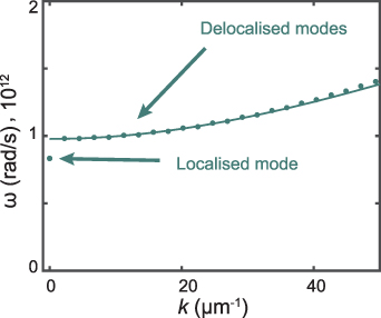
Figure 7. Spectra of spin waves modes calculated for the finite-size sample (dots) and infinite sample (solid line). The localized mode with k = 0 falls into the gap.
Download figure:
Standard image High-resolution imageBefore analyzing the magnetic dynamics of inhomogeneous samples, we briefly summarize some well-known results that can be obtained from the model in equations (1)–(4) for a single-domain sample. The magnon spectrum in this case consists of two branches of linearly polarized modes [7, 28], which we further refer to as a high-frequency (hf) and a low-frequency (lf) mode (see figure 2). The hf modes are polarized out-of-plane ( ), while the lf modes are polarized along the in-plane hard magnetic axis (
 ). An energy gap of mainly magnetoelastic origin [22, 23] at
  appears in the spectrum of both branches. The eigen-frequency at the center of the Brillouin zone amounts to
  for the hf branch and
  for the lf branch. In the long-wavelength limit (far from the Brillouin zone edge) the dispersion laws of both branches are similar, namely
  and
and  , correspondingly (see solid lines in figure 5).
Frozen spontaneous strain reduces the effective anisotropy of a single-domain state to an orthorhombic one, with two orthogonal hard axes  and
and  . Additionally, the strain-induced anisotropy stabilizes 180∘ domain walls, with the Néel vector rotating within the easy-plane between two opposite directions. Note that in the limiting case
  the 180∘ domain wall is unstable: pairs of 90∘ walls (film) or three 60∘ walls (bulk) form instead, since the dominant interaction becomes the magnetic anisotropy (which has a different geometry in bulk compared to thin films).
4. Linear effects
We now apply our model to two different physical multi-domain state configurations: two S-domains within one T-domain and two T-domains. Although only the latter case is relevant for optical experiments, as already demonstrated in the literature [43], we treat both scenarios to testify the generality of our modeling.
4.1. Two S domains, one T domain
Here we consider the generic case of an AF with a fixed orientation of an easy plane, which represents not only NiO, but also many other materials relevant for both the electric and the optical approaches to spintronics (for instance α-Fe2O3 [4], CuMnAs [8, 9], CoO [44], FeBO3 [45]). In the case of bulk NiO, we consider two S-domains belonging to the sameT-domain (we consider T1S1–T1S2) (see figure 6). In this case, the orientation of the hard out-of-plane axis,  , is fixed, and the out-of-plane anisotropy keeps the Néel vector in the easy plane inside both the domains and the domain wall. However, spontaneous strains introduce hard and easy in-plane magnetic axes, which are different in the S1 and S2 domains,
where ξ is the coordinate in the direction of the domain wall normal. In the case of a thin film, mutually orthogonal orientations of easy and hard axes transform into each other if the spatial coordinate ξ is inverted, i.e.  , when
  . It should be noted that the model in equation (5) relies on the assumption that the spatial profile of the spontaneous strains is described by a step function, whose discontinuity is located at the center of the domain wall in equilibrium. Possible variations of the strains due to the rotation of the Néel vector inside the wall are thus neglected. Such an approximation is acceptable if the domain size is much larger than the domain wall width.
By substituting equation (5) into equations (3) and (4) we find that the effective anisotropy in equation (2) is a space-dependent function. The profile of the domain wall in equilibrium, which is calculated from equation (1), is modified by the presence of the strain-induced field. For a thin film, the distribution of the Néel vector can explicitly be calculated, which reads
Here  is the width of the domain wall, which decreases as the magnetoelastic parameter
  increases. This is due to the fact that the magnetoelasticity contributes to the anisotropy, and thus increases the pinning of the Néel vector to an easy direction. In other words, although the orientation of the Néel vector (i.e. direction of the easy axis) is the same as in the absence of spontaneous strains, the magnetoelasticity makes the anisotropy potential well deeper. Calculations show a similar relation between the domain wall width and the magnetoelastic parameter also for the case of a bulk material. However, analytical expressions for this case are far from trivial.
In order to study the dynamics in the presence of the domain wall, we further calculate the spectra of the lf-magnon eigen-modes (symbols in figure 7), employing the methods described in section 3. Our simulations show that the spectrum consists of a continuum of delocalized modes (analogs of the plane waves in a single-domain sample) and one additional localized mode. The dispersion law ω(k) for the delocalized modes in a multi-domain sample (symbols) is indistinguishable from the case of a homogeneous system [46] (solid line). However, in contrast to the pure magnetic domain wall, the localized mode has a nonzero eigen-frequency,  , which lies in the energy gap of the magnon dispersion. The corresponding space distribution of the Néel vector can be approximated by the function
  (see equation (6)). As such, this mode is associated with the displacement of the domain wall center. Moreover, its frequency defines the value of the restoring force, which pins the domain wall to the center of strain inhomogeneity (ξ = 0) and scales as
  .
.
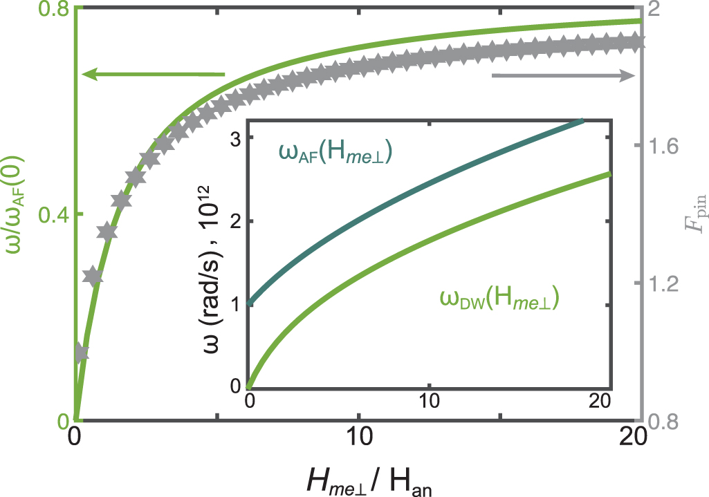
We calculated the frequency of the localized mode for different values of the magnetoelastic parameter (see figure 8), to gain insight into the role of the magnetoelasticity. In the limiting case of vanishing magnetoelasticity  the frequency tends to zero,
  . This is consistent with the absence of an activation barrier for a pure magnetic domain wall, as already mentioned in section 2. In the opposite limit (
 ), which is reliable for many easy-plane AFs (including NiO), the domain wall frequency tends to a finite value, namely
  , which is still below the continuum dispersion limited from below by the frequency of AF resonance
  .
.
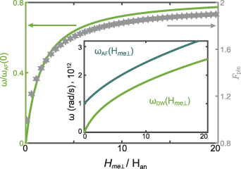
Figure 8. Frequency of the localized mode ( ), frequency of the magnon gap (
 ), and pinning force (
 ) as a function of magnetoelastic parameter
  .
.
Download figure:
Standard image High-resolution imageSince  is lower than the whole spectrum of the magnon continuum, an external stimulus perturbating the magnetic system at a frequency lower than
  can induce translational displacement of the domain wall with minor or negligible excitation of spin waves. This is similar to the mechanical model of a rigid body whose motion is not affected by the internal degrees of freedom (acoustic waves). In this case, the dynamics of the wall can be effectively described in terms of a collective coordinate. Here we consider as such a collective coordinate the position X of the domain wall center with respect to the center of strain inhomogeneity ξ = 0. Following a standard approach [25, 47], we substitute the equilibrium profile in equation (6) into the effective anisotropy in equation (2) and introduce the effective potential as
This effective potential corresponds to the energy cost related to the shift of the domain wall with respect to the frozen strains (see figure 1) and scales as  at
at  . We further calculate the pinning force
  as a maximal value of dU/dX (evaluated for
  ) (see figure 8, gray symbols). As is reasonable to expect, the pinning force increases with
  saturating in case
  .
.
The localized mode described above is associated with oscillation of the Néel vector within the easy magnetic plane and thus has the same polarization as the lf magnons. As such, and due to the pinning, lf magnons are reflected by the domain wall. Figure 9 shows the reflectivity coefficient R of the lf magnons calculated employing the Born approximation (see appendix  , the value of R growing with
  . Remarkably, the reflected magnons transfer momentum to the domain wall and thus can induce the domain wall oscillations.
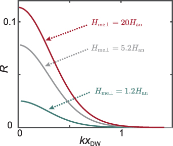
Figure 9. Reflectivity of lf magnons from the domain wall between two S-domains for different values of  . The reflectivity R is calculated as a function of
  in the Born approximation.
Download figure:
Standard image High-resolution imageWe would like to note that the described oscillations of the domain wall originate from the built-in strains, and the corresponding frequency is defined by the internal properties of the material. Another possibility to induce domain wall oscillations was recently considered [48]. The authors suggest applying a space-dependent external stress field, in which case the frequency of oscillations is controlled by the external parameters.
In the considered geometry, the hf magnons are disentangled from the dynamics of the domain wall, because of the orthogonality of their polarization vectors with respect to the orientation of the Néel vector in the wall. Moreover, their frequency is high compared to lf-magnons (figure 7), and thus they are almost insensitive to the presence of inhomogeneous strains. In the next section, we shall consider and thoroughly discuss a geometry in which the dynamics of hf and lf magnons are coupled.
4.2. Two Tdomains
In this section, we consider a domain wall separating two T-domains (see figure 3), which is typical for bulk NiO. This geometry has been recently addressed also experimentally [21]. In this case, all three vectors  are space-dependent, so that
The boundary between T-domains minimizes the energy of the magnetoelastic system if it is oriented along one of the directions, which satisfies the conditions of strain compatibility. We note that this condition is canonically termed as continuity of the displacement in elasticity theory and it follows from the continuous nature of the material described in the model. Such directions can be derived from symmetry considerations. Here we consider only such boundaries, since they determine the ground state of the materials experimentally investigated. As a consequence, the wall between the T1 and T2 domains is perpendicular either to the [100] or to the [011] direction (see appendix  is then defined as
Here we consider a sample consisting of two T-domains, T1S3 and T2S3 (referred further to as T1 and T2). Though the Néel vector in equation (9) is defined as a piecewise function, the exchange coupling through the interface between the T1 and the T2 domains imposes the additional condition  as shown in figure 3 (see appendix
We start from the description of the domain wall profile that is calculated using equations (1)–(3). In each T domain, the Néel vector rotates within the easy plane, so that  at
at  and
and  at
at  . The rotation within the easy-plane is then parametrized by means of the angle ϕ calculated from the equilibrium orientation within each domain
The equilibrium distribution ϕ0(ξ) is then given by the following equation
where we assume for simplicity that  . The parameter
  can be considered as the domain wall width.
We next turn to the discussion of the magnon dynamics in the presence of the T1–T2 domain wall. Let us start by considering the propagation of a linearly polarized spin wave ![$\delta\mathbf{n} = \mathbf{a}\exp\left[i(\omega t-k\xi)\right]$](https://content.cld.iop.org/journals/0022-3727/54/37/374004/revision2/dac055cieqn129.gif) . The polarization of the hf mode is
. The polarization of the hf mode is  , while the lf mode has a polarization given by the
  in the T1 domain (see figure 2).
The propagation through the T1–T2-interface must satisfy three conditions: (i) continuity of the Néel vector  at the interface; (ii) conservation of energy; and (iii) conservation of the linear momentum of the incoming and outgoing spin waves. From (i) it follows that the polarization vector
  has nonzero projections on both vectors
  and
and  , which results in the excitation of both in-plane and out-of-plane oscillations in the T2 region. In the case of high frequencies
  and
and  , if the incoming spin wave belongs to the hf mode in the T1 domain, the resulting excitations are the propagating waves with orthogonal polarizations along
  (hf mode) and
  (lf mode) and different wave vectors,
  and
and  , as it follows from condition (ii). This effect can be viewed as a magnonic analog of optical birefringence, in which a light wave impinges on a medium with polarization along the direction between the two optical axes. Consequently, the incoming wave is decomposed in the material into two components, each one polarized along one of the optical axes. Overall, the propagation of the wave inside the medium implies a rotation of its polarization vector, in comparison with the original incoming wave. In contrast, if
  and
and  (i.e. the incoming spin wave belongs to the lf mode in the T1 domain), the excited wave that is polarized along
  , is evanescent and thus localized, and may be related to the oscillations of the domain wall, as discussed in more detail below. Finally, taking into account conditions (i) and (iii) we anticipate a pronounced reflection of magnons from the T1–T2 domain wall, the reflectivity being
  for hf magnons and
  for lf magnons (neglecting small
  ). The lf mode is reflected in a more pronounced way because, given its lower frequency with respect to the hf mode, it interacts in a more pronounced way with the potential well represented by the wall.
These considerations show that in a multi-domain sample, the eigen-modes are polarized neither purely in- nor out-of an easy magnetic plane. Moreover, all the eigen-vectors have nonzero projections on both vectors  or
or  in each T-domain. If we also consider that the polarization of the modes is space-dependent (see figures 10 and 11), it is clear that a standard classification of the modes is hindered. In the case of a two-T-domain sample, we can rely on the orientation of the deflection of the Néel vector from the equilibrium orientations
  in the center of the domain wall (ξ = 0) as a criterion for the eigen-modes classification. Based on this, we distinguish between the modes with
  parallel to the domain wall normal (mode A, eigen-functions
  ) or the domain wall plane (mode B, eigen-functions
  ). The components of vector functions
  and
and  are either symmetric or antisymmetric with respect to inversion of
  and can be reduced to symmetric or antisymmetric combinations of the plane waves with opposite k vectors. As such, modes
  and
and  are degenerate as a consequence of the symmetry of the domain wall (permutation of the domains with inversion of ξ). Figure 10 shows the corresponding magnon eigen-frequencies (points) simulated for a finite-size sample with the following input parameters:
  ,
,  s−1, c = 105 m s−1 and von Neumann boundary conditions at the sample edges. We observe that the calculated frequencies of the lf mode deflect from the dispersion of a single-domain sample in the region where the magnons belonging to the lf and hf branches have comparable frequencies (see figure 5). This fact can be interpreted as a finite-size effect [49] which diminishes as the sample size increases. Numerical finite-size effects notwithstanding, the dispersion law coincides with the dispersion for a single-domain sample (solid lines), which allows us to keep the classification of the eigen-modes according to their frequency, k-vector and the mode type (lf or hf, A or B).
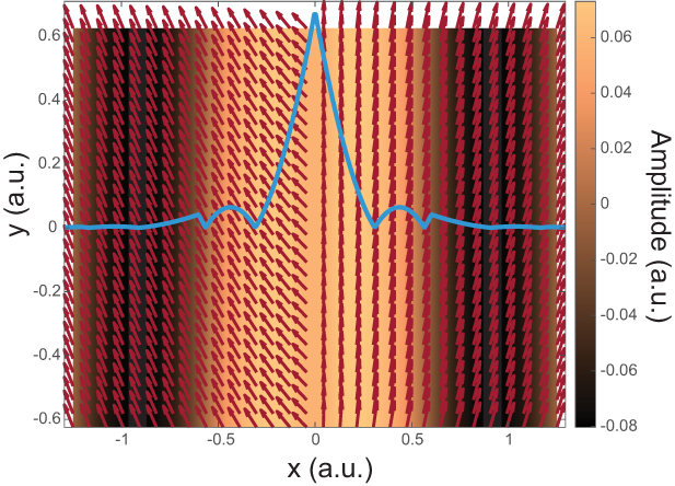
Figure 10. A hybridized magnon eigen-mode for two T-domains. The spatial distribution of the in-plane component (intensity color plot) and out-of-plane component (solid line) of the Néel vector in one of the lf eigen-modes. The arrows represent the Néel vector in equilibrium. On the scale of the figure the width of the domain wall amounts to 0.5.
Download figure:
Standard image High-resolution image
Figure 11. Components of an eigen-function  . The red line represents the in-plane component, while the blue line describes the out-of-plane component. The step-like variation of the out-of-plane component is an artefact of different coordinate systems in T1 and T2 domains, as expressed by equation (8).
Download figure:
Standard image High-resolution imageOur calculations confirm intuitive expectations that the eigen-modes of the lf branch include fully localized oscillations, as visually expressed by the space dependence of the out-of-plane (parallel to  ) projection of the eigen-functions
  and
and  , i.e. the out-of-plane component of the lf-mode (figures 10 and 11, blue line). The localization of the in-plane oscillations (parallel to
  ) is hidden due to hybridization with the delocalized mode, as can be seen from figure 11. The characteristic width
  of the localized contribution, whose space-dependence is well approximated by an exponential law
  , corresponds to the wave vector k of the delocalized spin wave (also used for the classification of the eigen-modes).
We associate such localized contributions with oscillations of the domain wall (for A-modes) or the domain wall width (for B-modes). However, in contrast to the case of the two S-domains considered above, the hybridized localized and delocalized modes and their frequencies reside in the continuum spectra of the lf branch. This means that the displacement of a domain wall is always 'dressed' with the cloud of delocalized magnons. Hence, the domain wall dynamics in terms of the collective coordinate X (position of the domain wall center) cannot be disentangled from excitation of spin waves.
The hybridization of the hf and lf modes at the T1–T2 interface affects the linear regime of spin dynamics, in terms of magnon birefringence and reflection. Nonlinear spin dynamics can be induced as well, as we discuss in the next section.
5. Nonlinear effects: parametric downconversion
In this section, we treat nonlinear spin dynamics, naturally arising in multi-T-domain samples. For this purpose, we consider again the propagation of a hf and low-k (k ≈ 0) spin wave ![$\mathbf{n}_\mathrm{in} = a\mathbf{e}_\mathrm{h\|}(T1)\exp[ i(\omega_\mathrm{hf}(k)t-k\xi )]$](https://content.cld.iop.org/journals/0022-3727/54/37/374004/revision2/dac055cieqn170.gif) impinging on the T1–T2 boundary. We focus on the dynamics of the Néel vector in the T2 domain (
impinging on the T1–T2 boundary. We focus on the dynamics of the Néel vector in the T2 domain ( ). Furthermore, we consider a small perturbation
  of the equilibrium solution
  (given by equation (10)) and rewrite equation (1) up to the second order in the excitations:
In these equations, the apices represent the spatial derivative with respect to the ξ coordinate (i.e.  ), δ(ξ) is the Dirac delta-function, and
  ,
,  .
.
We first consider a linear approximation of equation (12) by neglecting the terms in the second square bracket of the RHS. A natural basis for solving equation (12) is given by the orthogonal set of eigen-functions  (see section 4.2), so that
  . By projecting equation (12) on
  we get a system of independent equations for the amplitudes bk
(t) as
we get a system of independent equations for the amplitudes bk
(t) as

which we solve with the initial conditions bk
(0) = 0. Here τ is the relaxation time of magnons related to Gilbert damping. In the linear approximation, equation (12) describes the resonant excitation of the hf eigen-mode with frequency  and the nonresonant excitation of all other eigen-modes whose amplitudes vary as
Next, we disclose the nonlinear effects predicted by our model. As a concrete example, we describe the generation of the lf-mode with  and k ≈ 0 (further referred to as
  ) through a parametric resonance triggered by the driving mode with frequency and wave vector equal to
  . This process is described by the term in the blue box in equation (12) for the
  component. The conservation of energy dictates that the parametric downconversion can take place due to the mixing of the
  mode with the other lf mode with higher wave vector, i.e.
  . In this notation
  (see figure 12). We restrict our attention to a coupled system with the corresponding amplitudes
  and
and  and neglect possible coupling with the other modes:
where the coefficient
describes the coupling between the eigen-modes  and {ωk
, k}, the symbol
and {ωk
, k}, the symbol  denotes the tensorial product. The approximate approach in equation (15) is valid as long as the modes
  and
and  are well separated, so, we assume that k* is finite, i.e. far enough from 0.
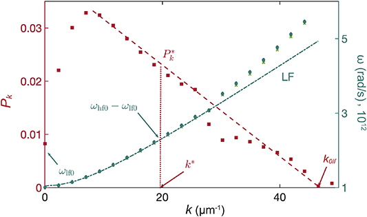
Figure 12. Excitation of lf mode magnons via parametric resonance. Left axis: modulus of the Pk0 coefficients. The red dash line is a linear approximation  . The vertical red dotted line marks the mode that participates in the parametric downconversion to frequency
  . The green dots and line show the eigen-frequencies of the lf modes (right axis). The kink in the wave vector-dependence of Pk0 is related to the finite-size effects (hybridization of lf and hf modes at the sample edges) and diminishes as the size of the sample increases. We ascribe the behavior at small k, which deviates from the linear approximation, to size effects, as the minimal value of k is limited by the sample size.
Download figure:
Standard image High-resolution image
The analysis of equation (15) shows that on top of the nonresonant excitations in equation (14), the driving mode induces an exponential growth of  and
and  as well,
  and
and  provided that the instability parameter fulfills the condition
Here we assumed that  .
.
The necessary condition in equation (17) for the parametric downconversion to occur includes the coupling coefficient  . This coefficient is proportional to the overlap of the in-plane components of the eigen-functions
  and
and  corresponding to the modes
  and
and  inside the domain wall, where the coefficient sin 2ϕ0 is nonzero, as shown in equation (16). In this region
  const and for
  the contribution to Pk0 from the delocalized, fast oscillating modes averages to zero, i.e.
  . The bottom line is that the main contribution to Pk0 originates from the localized oscillations. Figure 12 shows the calculated dependence of Pk0 on the wave vector, which can be fitted by a linear function
  in most of the plotted region. In the wave vector range
  both localized and delocalized components of the hybridized mode contribute to the signal, which gives rise to a maximum of Pk0 in this region. We thus conclude that the localized modes, or in other words the oscillations of the domain wall, mediate the coupling between the different eigen-modes and enable such nonlinear effects as parametric excitations. This phenomenon is consistent with the recently reported coupling of magnon modes in a multi-domain sample of bulk NiO [21]. Here we would like to highlight the role of the inhomogeneous strain field, which pins the domain wall and defines the landscape of the magnetic texture, thus enabling the coupling of the different eigen-modes.
6. Outlook
The results presented in this work can properly describe ultrafast spin dynamics in AFs considering boundaries between either S- or T-domains. Both cases are described, which grants our modeling a high level of generality, since most of the easy-plane AFs display these kinds of domains induced by magnetoelasticity. We aim to describe ultrafast spin dynamics, which naturally calls for the frozen lattice approximation. However, removing this approximation, while preserving the main structure of the modeling, can allow us to explore different physical regimes. To be more specific, we refer to:
- Spin dynamics in thin samples. If the size of the sample is so thin that the frequency of the acoustic waves becomes comparable with the spin wave frequency, the frozen lattice approximation does not hold anymore. The evolution of the strain fields takes place on the same timescale as the spin dynamics and it has therefore to be taken into account. We can envisage an experimental set-up, in which such an effect can be investigated. A well-established scheme, consisting of a metallic transducer sputtered on top of the magnetic material, is typically employed to launch strain acoustic waves into the magnet [50, 51]. Applying this scheme to AFs is expected to disclose exactly the regime of combined lattice and spin dynamics on the picosecond timescale.
- Excitation of hybridized magneto-acoustic waves. In some magnetic materials, the dispersion of magnons and phonons display avoided crossing for certain wave vectors, which indicates the formation of a hybridized wave. This problem has already been addressed on the ultrafast timescale [52, 53], but neither in single- nor in multi-domain AFs.
- Polaritons. Under certain conditions, such as small defect-induced pinning and rather pronounced magnetostriction, a combined excitation of the lattice and of the domain wall motion (i.e. not magnons) can be induced. The effect of such hybrid excitations on the spin dynamics of the material can then be explored with our model.
- Nanosecond (or longer) spin dynamics. The (sub)-picosecond regime of spin dynamics is relevant for all-optical experiments. However, extensive research activity explores spintronic concepts in AFs by means of transport methods. These techniques can access nanosecond or longer time-scales, which cannot be described relying on the idea of a frozen lattice. Thus, employing our model beyond this approximation, the spin dynamics investigated by transport techniques in multi-domain AFs can be described.
- External modification of strains. In our model, we consider only spontaneous strains, which are thus internal to the material and do not evolve in time. However, strain can be externally induced mechanically. The evolution of the strain configuration, and its subsequent effects on the spin dynamics in multi-domain AFs can be addressed with our model by removing the frozen-lattice approximation.
7. Conclusions
Our work reports a phenomenological model able to portray the effect of domain walls in the presence of magnetoelasticity on the equilibrium and dynamical properties of AFs. First, we calculated the equilibrium magnetic configuration, showing that the magnetoelasticity pins the domains, also in the absence of defects, establishing de facto the domain structure. We then calculated the spectrum of magnons and of the eigen-modes of the domain wall, both S and T, showing that they are significantly different, which has implications for the spin dynamics itself. Consequences of the domain walls in both linear and nonlinear regimes of spin dynamics have been computed and found to be consistent with recent experiments [21].
The ability to treat both S- and T-domains widely extends the applicability of our theory. Additionally, we have provided multiple examples of what can be achieved by further developing our modeling. Our work has the potential to be a milestone in the development of a platform to shed light on promising routes for sample engineering. Using hypothetical sample parameters as input (domain size, acoustic properties, magnetoelastic tensor), the huge iceberg of magnetic nonlinearities, which were considered solely at the lowest order in the present work, can be extensively explored with our model, which can then provide feedback for material design and development.
Acknowledgments
D B acknowledges support from the Deutsche Forschungsgemeinschaft (DFG) Program BO 5074/1-1 and BO 5074/2-1. O G acknowledges support from the Alexander von Humboldt Foundation and by the Deutsche Forschungsgemeinschaft (DFG, German Research Foundation)—TRR 173–268565370 (Project A11), TRR 288–422213477 (Project A09), and Project SHARP 397322108.
Data availability statement
All data that support the findings of this study are included within the article (and any supplementary files).
Appendix A
A.1. Magnetic and magnetoelastic energy of NiO
In this section we introduce the magnetic and magnetoelastic energy of NiO, based on symmetry considerations.
The antiferromagnetic structure of NiO is formed by the ferromagnetically ordered (111) planes stacked in an alternating order [30, 31, 33]. Phenomenologically, this magnetic structure is described by a multi-dimensional order parameter given by a set of four Néel vectors,  , as it is usually introduced based on symmetry considerations [32]. Each
  is associated with one of four arms
  of a star
 ![${\mathbf k}_9 = [{1\over{2}} {1\over{2}} {1\over{2}}]$](https://content.cld.iop.org/journals/0022-3727/54/37/374004/revision2/dac055cieqn212.gif) that corresponds to the two-dimensional irreducible representation τ6 (in Kovalev's notations [25]) of the space symmetry group
that corresponds to the two-dimensional irreducible representation τ6 (in Kovalev's notations [25]) of the space symmetry group  of the paramagnetic phase. We use the following notations for the four arms of
  :
:
Expressions for the magnetic and magnetoelastic energy are constructed as invariant combinations of the order parameters  and strain tensor components uij
. The general expression for the magnetoelastic energy reads
and strain tensor components uij
. The general expression for the magnetoelastic energy reads
Here Λ is a magnetoelastic constant of exchange origin, while λij are relativistic magnetoelastic constants in Voigt notations, the coordinate axes x, y and z are aligned along the cubic crystallographic directions [100], [010], and [001].
As each type of T domain, Tp, is associated with only one structural vector  and only one Néel vector
  , we consider further the T1 domain and assume that out of four Néel vectors only
  .
.
Assuming that in equilibrium ![$\mathbf{n}\|[11\overline{2}]$](https://content.cld.iop.org/journals/0022-3727/54/37/374004/revision2/dac055cieqn219.gif) we calculate spontaneous strains by minimizing
we calculate spontaneous strains by minimizing  , where the density of the elastic energy reads
Minimizing of the expressions (3) and (4) gives the following values of the spontaneous magnetostriction in the T1S1 domain:
Here Ms
/2 is the sublattice magnetization. The largest, parameter  (
( ) corresponds to contraction along [111] axis and it is associated with the rhombohedral distortion induced by the magnetic ordering. Two other parameters
  ,
,  (
( , see, e.g. [40]) are associated with the orthorhombic deformation. The isomorphic striction,
  corresponds to the volume change during the transition and is negligibly small.
The approximation of frozen strains implies that the spontaneous strains once formed do not participate in magnetic dynamics. The corresponding contribution into the magnetic energy is then obtained by substituting equation (A4) into equation (A2). For the T1 domain this gives
Here we neglected small components  and
and  . By rotating the coordinate system from the cubic axes to the coordinate vectors
  we reduce equation (A5) to equation (2), where
The first term in equation (A5) is of an exchange nature and as such, does not depend on the orientation of the Néel vector. However, it defines the transition region between different order parameters  at the interface, as will be shown in the next section.
A.2. Continuity of the order parameter at the interface between two T domains
In this section we consider an interface between the domains T1 and T2 (a similar consideration applies for any pair of T domains) with the order parameters  and
and  , respectively. Within the domain boundary local spin vectors are represented as a superposition of two order parameters:

The normalization conditions  impose the additional relation
  ,
,  .
.
To calculate the space dependence of the order parameters inside the domain wall we consider the following contributions into the energy density:
where ξ is coordinate along either the [100] or the [011] crystallographic direction, A parametrizes the inhomogeneous exchange coupling, and the last term in equation (A8) has magnetoelastic origin (see equations (A2) and (A5)). Assuming that inside the transition region the orientation of the vectors  and
and  is fixed, we find that the energy (A8) is minimized by the following space distribution of the order parameters:
As  , we conclude that the thickness of the transition region, where the order parameter changes from
  to
to  , is much narrower than the domain wall width considered in the main part,
  . So, we can introduce the Néel vector that continuously varies between two T-domains, see equation (9).
A.3. Calculation of scattering coefficient for Sdomain wall
In this section we calculate the reflectivity of the spin-waves at the pinned domain wall. We consider the 90∘ domain wall whose equilibrium profile is given by equation (6) of the main text, with the Néel vector rotating within the easy plane. We parametrize the Néel vector with the spherical angles ϑ and ϕ, so that

We set ϕ = ϕ0(ξ)+δϕ(ξ, t) and ϑ = δθ(ξ, t), where ϕ0(ξ) is an equilibrium solution (given by equation (6)) of equation (1), δϕ and δθ correspond to in-plane and out-of-plane excitations, respectively. The linearized equation (1) then reads as
where θ(ξ) is the Heaviside step-function. Operator  appears in the Pöschl and Teller problem [54] and includes nonreflecting potential, whose eigen-functions are well-known:
We then consider  as a scattering potential and apply the Born formula to calculate scattering of an incoming wave
  :
:
where
is the Green function of operator  (see, e.g. [55]). Taking
  , we obtain from equation (A15) the following expression for the reflection amplitude r:
The reflectivity shown in figure 9 is then calculated as  .
.
A similar procedure can be applied for the calculation of the reflection coefficient for the out-of-plane waves, for which one should consider the second of equation (A11). However, as  , the contribution of scattering potential
  into the dynamics of spin waves can be neglected. In this case R ≈ 0.