

Abstract
A new diagnostic approach using multi-mode microwave cavity resonance spectroscopy (MCRS) is introduced. This can be used to determine electron dynamics non-invasively in an absolute sense, as a function of time and spatially resolved. Using this approach, we have for the first time fully mapped electron dynamics specifically during the creation and decay of a highly transient pulsed plasma induced by irradiating a background gas with extreme ultraviolet (EUV) photons. In cylindrical geometry, electron densities as low as 1012 m−3 could be detected with a spatial resolution of (sub)100 µm and a temporal resolution of (sub)100 ns. Our experiments clearly show production of electrons even after the in-band EUV irradiation fades out. This phenomenon can be explained by both photoionization by out-of-band EUV radiation emitted by the EUV source later in time and delayed electron impact ionization by electrons initially created by in-band EUV photoionization. From the analysis, the absolute width of the electron cloud in the probing volume could also be retrieved temporally resolved. This data clearly indicates cooling of electrons. From an application perspective, it is demonstrated that the method can be used as a non-invasive and in-line monitor for ionizing radiation in terms of beam power, profile and pointing stability.
Export citation and abstract BibTeX RIS
1. Introduction
The most essential step in the production of semiconductor circuits is photolithography. This multi-billion-dollar industry consistently adheres to Moore's law in printing an increasing number of transistors on a single chip. The smallest possible feature to be printed is dictated by the numerical aperture (NA) of the system and the wavelength of the light used [1]. By scaling both, in recent decades scientists and technologists have successfully reached multiple industry-driven milestones. These include the introduction of immersion photolithography (increasing the NA of the system) and shortening the wavelength used. By far the most challenging step in this industry, however, is only now being taken: the introduction of extreme ultraviolet (EUV) lithography [2] at a wavelength of 13.5 nm. Besides the extreme conditions needed to generate EUV photons, the full system requires a working pressure which is as low as possible in order to minimize photon absorption by background gas. Although the background conditions correspond to ultra-high vacuum, the system still requires a controlled amount of gas to be permanently present.
Inevitable when sending pulsed bunches of highly energetic (92 eV) photons through a gas—as low as its pressure might be—is the creation of an exotic type of plasma. This peculiar phenomenon is called EUV photon-induced plasma [3]. Not only is this kind of plasma highly transient in time, but the electron energy distribution is initially far from Maxwellian, with energies sufficiently high to produce even more plasma by means of electron impact ionization. Despite its relevance in outer space, research on the physical properties of EUV photon-induced plasmas has been scarce in literature. With the introduction of EUV lithography, however, several groups worldwide have now picked up this research topic. The reason for the industrial interest is that these plasmas will inevitably impact the operation of lithography tools in terms, for instance, of cleaning and the lifetime of delicate optical and other components [4–11].
EUV photon-induced plasmas have been modelled numerically by, for example, Abrikosov et al [12] and Astakhov et al [13]. From an experimental point of view, literature is scarcer, mainly because of the limited availability of the few and very expensive EUV-producing light sources. Experimental characterizations of EUV photon-induced plasma include monitoring the temporal evolution of the electron density [14–19] and studying the impact of ion fluxes on surfaces [20, 21].
In particular, studying the dynamics of the cloud of free electrons generates possibilities to reveal fundamental processes regarding plasma creation, plasma expansion, thermalization of the plasma and the dynamic formation of space charge regions, including their governing electric fields. Up until now, this electron density evolution has only been studied successfully using a non-invasive diagnostic called microwave cavity resonance spectroscopy (MCRS). Other traditional electron diagnostics such as Thomson scattering and the utilization of electric probes have appeared non-feasible under these conditions. For instance, the density of free electrons is far too low for Thomson scattering to deliver a sufficient signal [22], while van de Velden et al [23] showed back in 2008 that the use of electric probes was problematic for diagnosing photon-induced plasmas. Although absolute values for the density of free electrons could be retrieved from MCRS measurements [14–19], results have always been averaged over the full experiment volume and not corrected for the local electric field value of the resonant mode used. Hence, spatial information could not be retrieved using traditional MCRS. Only one experimental paper exists [16] in which the authors determine full-width-at-half-maximum (FWHM) values of spatial electron distribution functions by taking into account two resonant modes. Although a part of the electron dynamics could be described by these experiments, the results were not quantitative and not corrected for the electric-field component of the microwave resonant modes used.
The novelty of this article is threefold.
- A novel diagnostic approach is developed and introduced, making traditional MCRS spatially resolved and electric-field corrected for the first time since its introduction in the 1950s [24].
- The electron dynamics in a highly transient plasma such as an EUV photon-induced plasma are both spatially mapped and temporally resolved, revealing new insights into plasma dynamics.
- From an application point of view, it is demonstrated how multi-mode MCRS can be applied as a beam power, profile and pointing stability monitor.
2. Method
2.1. MCRS principle
From a historical perspective, MCRS is based on a series of publications from the 1950s [24–26]. The last of these, in particular, proposes the use of interaction between electromagnetic fields in the microwave frequency regime and plasmas to probe the density of free electrons. Ever since, MCRS has been further developed and used to investigate the properties of many types of plasma. For instance, to measure the density of electrons in low-pressure radiofrequency-driven gas discharges [27]. In concert with laser-induced photodetachment, MCRS has even appeared to be an advantageous diagnostic to measure the density of negative ions in, for instance, etching plasmas [28–30] and powder-forming plasmas [31–34]. Since 2015, MCRS has been used to study the highly transient phenomena in plasmas generated by the irradiation of gas by ionizing (EUV) photons [13–15, 17–19, 35]. Full theoretical considerations regarding the MCRS technique have been described extensively in literature [27]. In this section, the working principle of this diagnostic is explained by mentioning only its key aspects. Readers are referred to the aforementioned literature for more details and mathematical background.
The essence of MCRS is that the plasma under investigation is produced inside a cylindrical pillbox cavity. The geometry of this cavity is designed such that resonant modes can be excited at resonance frequencies in the microwave (MW) range (a few GHz). The exact frequency at which a certain resonant mode exists is defined mainly by the geometrical configuration of the cavity (which is fixed during experiments) and the permittivity  of the medium inside the cavity. For a fixed cavity, multiple resonant modes may exist over a certain frequency range. Two types of resonant modes are usually recognized: transverse electric, TEmnp, and transverse magnetic, TMmnp, with m = 0, 1, 2, ... (for TE: m = 1, 2, 3, ...), n = 1, 2, 3, ... and p = 0, 1, 2, ...).
The quantitative diagnostic approach of MCRS is based on the fact that the presence of free charge carriers (in this case plasma) directly gives rise to a finite increase in  r as [30]
In this equation, the term  (with i the imaginary unit) accounts for losses due to non-idealities of (or in) the cavity while the collision frequency
  between electrons and other particles—which is usually considered as a loss term as well—is negligible in our case due to the low gas and electron densities. As will be described later in this article, the quality factor 'Q' is a measure of the rate at which a cavity can be loaded or reloaded with microwave energy and therefore determines the response time of the diagnostic under discussion. As can be seen in equation (1), r depends on the angular frequency
  of the microwave field used and the electron plasma frequency
  given by:
where  and
and  are the mass of an electron and the elementary charge respectively, and
  the permittivity of vacuum. The diagnostic force becomes immediately clear when we realize that the electron plasma frequency—and therefore r as well—is directly affected by the electron density
  .
.
Since the diagnostic is operated in the microwave regime, the inertia of ions and heavier charge carriers (e.g. nanometre and micrometre-sized particles) is too large to allow these particles to follow the electric field oscillations. Unlike ions, electrons are sufficiently mobile to follow the microwave fields applied and therefore to determine the permittivity of the plasma.
Overall, compared with the situation in vacuum, the presence of free electrons inside the cavity affects , while in turn affects the resonance frequency  of the resonant mode used. In the diagnostic presented here, a lossless and isotropic cavity medium with permittivity
  and permeability
  is assumed. This means that the electric field E and electric displacement field D of a resonant mode are related by
  . For the magnetic fields, a similar relationship holds:
  . The current application focuses on unmagnetized low-pressure and non-thermal plasmas, for which it is common to assume
  and that the ions are immobile and cold. It can be derived from [36] that the electric-field-averaged electron density
  inside a cavity relates to the resonance frequencies f0 and f of a specific resonant mode in an empty cavity and in a cavity partly or completely filled with free electrons, i.e. plasma, respectively as:
with  the resonant frequency shift due to the presence of plasma. Note that
  is an electric-field-averaged electron density taking into account both the spatial distribution of the free electrons over the cavity volume
  and the local value of the electric-field component
  of the MW resonant mode.
This means that, depending on the resonant mode used, electrons at different positions in the cavity are probed to a different extent. Hence, MCRS yields electron densities which are inherently cavity-averaged and electric-field weighted.
Until now, this has always been experienced as a disadvantage of the MCRS technique. However, the analysis and comparison of multiple modes can serve to resolve the electron density distribution spatially. Successful application of this method is demonstrated in the current article.
2.2. Multi-mode MCRS
As already mentioned in the previous section, the extent to which free electrons are probed by the MCRS diagnostic scales directly with the local value of  of the specific resonant mode. Hence, the resonance frequency shift
  induced by the local presence of electrons is different for each resonant mode. Six examples of computed
  components of different resonant modes in an ideal cylindrical cavity are given in figure 1.
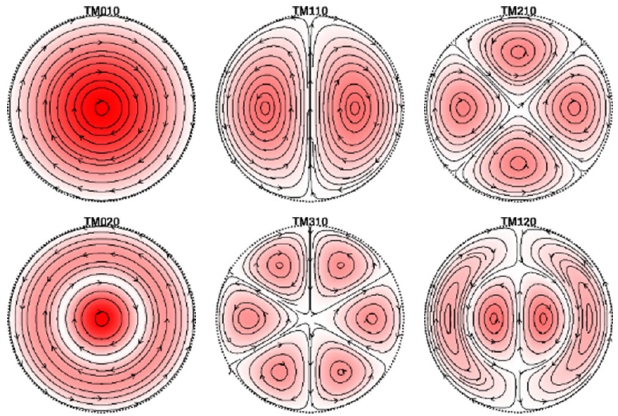
Figure 1. Analytically computed electric-field distributions (red is a high electric field magnitude, white a low electric field magnitude) and magnetic field lines (arrows) for several possible resonant modes in an ideal cylindrical cavity (dashed). The axis of symmetry (z) is pointing away from the paper.
Download figure:
Standard image High-resolution imageTaking into account equation (4), it can be reasoned that electrons present on the axis of this cavity are probed with a high weighting factor (large  ) by the resonant TM010 and TM020 modes because
  is at its maximum on the axis. At the same time, the same electrons are hardly detected by the other modes shown in figure 1 because these show
  on the axis. It is precisely this difference in the spatial sensitivity of the different resonant modes to the presence of free electrons which is used to make multi-mode MCRS spatially resolved. The procedure to achieve this is elaborated in the following section.
2.2.1. Reconstruction of electron density distribution profile.
To obtain spatially resolved electron density profiles, MCRS is applied in N resonant modes and for each time step and resonant mode the shift in resonance frequency  ;
;  ; ... ;
  caused by the presence of free electrons is measured. From these values, the cavity-averaged and electric-field-weighted electron densities
  ;
;  ; ... ;
  can be calculated using equation (3). For each
  combination of resonant modes
  , the ratio between the respective
  and
and  values is determined as
  . In parallel, from a theoretical perspective, the similar ratios
  are determined by assuming a certain spatial ne profile shape. Corresponding with measurements of the intensity profile of the initial irradiation profile (see figure 12(b)), a Gaussian profile has been considered here. However, it should be noted that every other possible profile shape (e.g. Bessel-like) might and can be used if the actual plasma physical situation demands so.
The reconstructed profile corresponds with the smallest root-mean-square error  between
  and
and  ,
,
which is brute-force calculated over a range of centre positions  and widths
  of the 2D Gaussian electron density profiles,
Note that, since the modes used in this work all have field components which are axially independent (despite small deviations close to the entrance and exit holes of the cavity), and also the xy intensity profiles of the beam used does not change along the z-direction inside the cavity,  is independent of z.
This reconstruction procedure can be run for each time step for which experimental data for  ;
;  ; ... ;
  is available. Therefore, the output of the reconstruction method we have developed in-house is the centre position (
 ,
,  ) of the maximum of the electron density profile and its width σ(t) with—in the case of reproducible plasma events—a temporal resolution limited by the Q of the cavity and the resonant mode used. The spatial resolution (of the reconstruction algorithm) of the centre position is 100 µm and that for the width is 10 µm. Volume integrals are calculated numerically, with electric fields and electron densities averaged along the axis of the cavity (z-axis) since we are only interested in and calculate 2D
  profiles (equation (6)),
where  is the number of grid points in the xy-plane and
  the constant spacing of the grid points in both the x- and y-direction; and
where  is the number of grid points in the z-direction.
For  , fields simulated with CST Microwave Studio (see appendix A for detailed information and the computed E-field profiles) have been used as input. Furthermore, it is assumed that the electron density is zero outside the probing volume (see figure 3).
2.2.2. Restoring absolute values.
Since the reconstruction algorithm optimizes 
 and σ for the smallest value of
  , the maximum value of the profile
  is lost and has to be determined during post-processing. To this end, equation (4) is solved for
  but now using the reconstructed 2D ne profile (with numerical approximations similar to those above),
where  signifies a certain resonant mode. Irrespective of the combination of modes used for the reconstruction,
  is calculated for all N modes that show good agreement between experimentally determined E-field profiles using the bead-scanning method (see appendix B) and the ones simulated using CST Microwave Studio (see appendix A). Subsequently, the mean value
  and standard error
  associated with it is calculated as
where  is the uncertainty on each value. The 95% confidence interval of
  is given by roughly
  .
.
3. Experiment
3.1. Experimental configuration
The experimental configuration used is depicted schematically in figure 2. Mechanically, broadly speaking the setup consists of three chambers: the source chamber, the collector chamber and the measurement chamber. The radiation source—housed in the source chamber—is a discharge-produced pinch plasma in xenon gas, producing pulsed radiation including contributions with wavelengths in the EUV range. All the features of this source have been described extensively in [14, 37]. In the configuration used, the pulsed radiation produced by the EUV source has a repetition rate of 500 Hz, a pulse duration of roughly 100 ns and a pulse energy of 125 µJ in the 10–20 nm wavelength range.
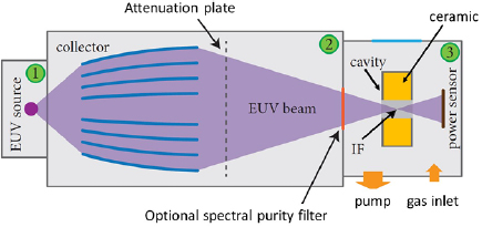
Figure 2. Schematic representation of the experimental setup used, with (1) the source chamber housing the EUV source, (2) the collector chamber housing the collector, an attenuation plate and, optionally¸ a spectral purity filter and (3) the measurement chamber housing the resonant cavity. The collector focuses the EUV beam in the intermediate focus (IF). Adapted with permission from [37]. Copyright © 2015 R. M. van der Horst.
Download figure:
Standard image High-resolution imageThe collector chamber (1.5 m in length and 1 m in diameter) houses the collector, which is a set of grazing-incidence multilayer mirrors in 'Wolter' configuration (aligned in an 'onion-like' structure) as described in, for instance, [38]. This collector focuses the light emitted by the EUV source in the intermediate focus IF in the measurement chamber. In the IF, the beam waist is approximately 4 mm and the beam has a divergence of 10° [37]. Although this setup has the option to install a spectral purity filter between the collector and the measurement chamber, none was used during the experiments presented here. The measurement chamber houses the microwave resonant cavity through which EUV photons can be directed without releasing any electrons from the walls by photoelectric effects. The spectrally integrated EUV power is monitored by a thermal EUV power sensor with an experimental error of 6% [37].
3.2. Cavity design
A schematic diagram and a photograph of the cylindrical cavity developed for this work are provided in figure 3. The base of the cavity is an aluminium body with a screw-on brass lid. Fully mounted, the inner diameter of the cavity is 29 mm and its inner height is 15 mm. Two concentric holes in the brass lid and in the base of the cavity, aligned at the cavity axis, allow irradiation of the gas inside with EUV photons without creating photoelectrons from the cavity walls. These photon entrance and exit holes both have a diameter of 10 mm. Based on the work of Lassise et al [39, 40] on making small and power-efficient cavities, the cavity is partly filled with a ZiTiO4 ceramic between a radius of 5 mm and 12.5 mm. This ceramic from T-CERAM ('E-37') was chosen for its low loss term  and its high
  (at 10 GHz) [40]. Whilst using a material with a low loss term is largely relevant for these applications, a high
  could be advantageous for two reasons. First, the high permittivity makes the cavity larger in a virtual sense, meaning that the resonant modes used can be excited at lower resonant frequencies. This in turn means that the holes in the lid and base can be drilled larger without causing significant 'leakage' of microwave radiation from the cavity. Second, the mode shows field concentration around the axis of the cavity while the ratio between the volume with which plasma is created by the EUV irradiation and the total cavity volume is also much larger. This combination results in a significant improvement overall in the signal-to-noise ratio of the diagnostic. It is impossible to neatly drill a small hole in the ceramic, so it was decided instead to position the (straight) antenna used to excite the MW modes outside the ceramic material, very close to the inner cavity wall. To keep the ceramic in place, a Teflon centring ring fills the gap between the cavity wall and ceramic (between a radius of 12.5 mm and 14.5 mm). The antenna used, which slides into the slot in the Teflon ring, is a straight and fixed piece of copper wire (diameter 1 mm, length approximately 20 mm) connected to the MW source by a fixed SMA feedthrough. To be able to heat the cavity to a set temperature (and keep it stable there), the aluminium housing includes four slots housing cartridge heaters and one slot that can house a Pt1000 temperature sensor. It also has four M4 holes in the outer side wall (at half height), to be able to fix it in the setup.
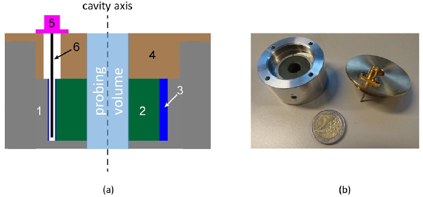
Figure 3. Schematic diagram (a) and photograph (b) of the basic cavity design with (1) aluminium cavity base, (2) ceramic with relative permittivity of approximately 37 in the MW regime, (3) Teflon centring ring with a slot in the axial direction for the MW antenna, (4) brass cavity enclosure, (5) SMA connector, and (6) straight MW antenna. The cavity base contains slots for housing cartridge heaters and Pt1000 temperature sensors.
Download figure:
Standard image High-resolution image3.3. Data-acquisition hardware
A schematic diagram of the acquisition system is provided in figure 4. Unlike past MCRS measurements by the EPG research group, which used two loop antennas as a sender–receiver pair for transmission measurements, ours are performed in reflection mode using a single straight antenna. A microwave generator (Stanford Research Systems SG386) produces a sinusoidal microwave signal at 16 dBm power and at a frequency set by the PC. This output is connected to the output port of a directional coupler (Mini-Circuits ZHDC-10-63-S+) and in principle passes unhindered to its input port, which is connected to the antenna inside the cavity. In this way, resonances can be excited in the cavity by applying the correct output frequency from the microwave generator. If the cavity is off resonance, power coupling to it is very inefficient and most of the power reaching the antenna reflects back to the microwave generator, where it is dissipated. Part of this signal (10%), however, is rerouted by the directional coupler to the measurement leg of the detection system, where it is first converted to DC by a logarithmic power detector (Hittite 602LP4E, 10 ns rise and fall time) and subsequently fed to a high-frequency (up to 250 MHz, but for the current measurements set to 50 MHz) transient recorder (Spectrum M3i.4121-exp) inside the same PC. The transient recorder continuously samples its input port and stores the data in its internal memory. Only upon an external TTL trigger, for which the trigger signal produced by the EUV source related to the discharge between the electrodes is used, is data made available to the user for subsequent analysis. This arrangement allows us to analyse part of the signal before the actual trigger occurs. If the cavity is at resonance, hardly any signal reflects back (most of the energy is dissipated in the electromagnetic field inside the cavity) and that probed by the transient recorder is low. Data analysis is similar to that discussed in previous work [33, 37, 41, 42], differing only in the 'direction' of the resonance peaks (maxima versus minima, see figure 5).
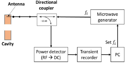
Figure 4. Schematic diagram of the data-acquisition system.
Download figure:
Standard image High-resolution image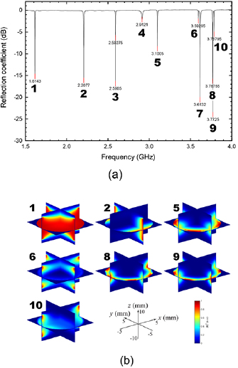
Figure 5. (a) Response of the developed microwave resonant cavity as a function of excitation frequency in the range 1.5–4.0 GHz; (b) simulated electric-field profiles in the probing volume of the cavity used for further multi-mode MCRS analysis.
Download figure:
Standard image High-resolution imageDuring the measurements presented in this paper, the microwave source was set to a certain frequency and kept at this frequency during the entire duration of the EUV pulse and the measurement time after this pulse. Just before the gas in the cavity is exposed to the next EUV pulse, the microwave source is set to the next value. To obtain sufficient accuracy, a resonant peak is probed by measurements at 25 different frequencies located in the frequency domain closely around the resonant frequency.
3.4. Calibration and characterization of the cavity
In order to translate the measurements taken into quantitative results, (i) each resonant mode has to be identified and (ii) the electric-field profile of each resonant mode used must be spatially resolved in a known manner. To this end, the electric-field profiles are obtained in two ways: numerically, using the commercially available Microwave Studio simulation package (see appendix A), and experimentally using the 'bead-scanning' method (see appendix B).
Figure 5(a) shows the cavity-response spectrum in the frequency range 1.5 to 4.0 GHz. In this spectrum, 10 resonant modes can be identified. But only those (modes 1, 2, 5, 6, 8, 9 and 10) for which the electric-field profiles obtained by the bead-scanning method and from CST Microwave Studio show reasonable agreement are taken into account for further multi-mode MCRS analysis. As an example, figure 6 shows the experimentally and numerically determined field profiles for the first two modes; results for the others used can be found and compared in figure C1 in appendix C.
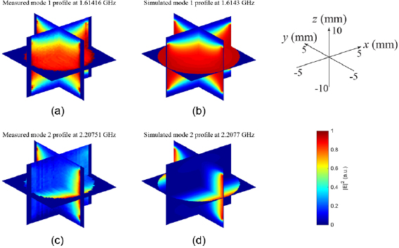
Figure 6. Electric-field profiles obtained experimentally using the bead-scanning method (a), (c) and simulated using the CST Microwave Studio package (b) and (d), for modes 1 (a), (b) and 2 (c), (d). Results from the bead-scanning method correspond well with the simulations.
Download figure:
Standard image High-resolution imageFigure 5(b) shows those (simulated) electric-field profiles in the cavity probing volume to be used for further analysis.
In MCRS in general, the Q-factor (or 'Q') is a crucial parameter when it comes to limitations in terms of resolution in time and accuracy in  determination. This factor is defined as the ratio between the energy stored in the cavity and the energy dissipated per cycle due to non-idealities. It can be deduced from the measured FWHM Γ and the frequency f at which this resonance curve shows its maximum
The higher the 'level of perfectness' or Q of a cavity, the more energy can be stored in it and the lower the energy-dissipation rate due to imperfections. This means that cavities with a high Q have a narrow resonance curve which results in accurate determination of  . At the same time, a high Q results into a slow response by the cavity to changes in permittivity and hence in
  . The 1/e response time τ of the cavity relates to Q and resonance frequency of a specific resonant mode as:
In practice, when designing a cavity one should tweak Q in order to find a suitable optimum between accuracy in  determination and the time resolution of the diagnostics. The resonant modes of our cavity have Q's listed in table 1 together with the corresponding cavity response times, which are in the order of 100 ns.
Table 1. Resonance frequency f0 and FWHM Γ, together with the resulting Q and cavity response time, for each of the resonant modes of the cavity developed in this work.
| f0 (GHz) | Γ (MHz) | Q | τ (ns) | |
|---|---|---|---|---|
| Mode 1 | 1.610 | 3.12 | 517 | 102 |
| Mode 2 | 2.209 | 4.73 | 467 | 67 |
| Mode 5 | 3.104 | 4.43 | 701 | 72 |
| Mode 6 | 3.594 | 2.60 | 1382 | 122 |
| Mode 8 | 3.771 | 2.83 | 1333 | 112 |
| Mode 9 | 3.776 | 3.30 | 1144 | 96 |
| Mode 10 | 3.788 | 2.19 | 1730 | 145 |
The current diagnostic has a huge dynamic range but still is limited. For instance, the lower detection limit is noise-determined. The upper detection limit of MCRS is determined by the moment at which the perturbation theory of Maier and Slater [43] is no longer valid ( ). The lower detection limit has—up until now [14, 15, 18, 19]—been demonstrated to be in the order of 1013 m−3, while in our work the sensitivity is improved by one order of magnitude. The upper detection limit is 1018 m−3. Expected values of
  in the EUV-induced plasma under the current conditions are between the lower detection limit and 1016 m−3. Hence, MCRS is a suitable diagnostic for studying this kind of plasma system.
4. Results and discussion
Multi-mode MCRS has been applied to a highly transient plasma induced by irradiation of a residual background gas at 10−4 mbar with pulsed EUV radiation. The cavity geometry used is as introduced and discussed in 3.2. The results and discussion presented in this section are divided into three parts. Section 4.1 demonstrates the multi-mode MCRS method through the generation of absolutely calibrated electron densities from traditional MCRS measurements using different resonant modes. Section 4.2 uses these multi-mode MCRS measurements to reveal new physical insights into the dynamics of EUV-induced plasmas. For instance, unexpected phenomena such as additional electron production even after extinguishing of the main EUV pulse have been observed, an effect which can be explained by the presence of unfiltered radiation from the xenon-pinch-discharge EUV source and the governing interaction of this radiation with gas. Finally, section 4.3 demonstrates that (and how) multi-mode MCRS can be applied as a non-intrusive in situ beam power, profile and pointing stability monitor for ionizing radiation [44].
4.1. Multi-mode MCRS: from volume averaged to 'real' electron densities
The cavity-averaged and E-field-weighted density of free electrons  obtained from traditional MCRS using different resonant modes is depicted on the left-hand side of figure 7 as a function of time before and after irradiation of the gas with a pulse of EUV photons. On the right-hand side are shown simulated electric-field profiles through the whole cavity volume (including the ceramic and Teflon) for each of these resonant modes. Note that modes 8 and 9 are basically identical, with the only dissimilarity being that their axes of symmetry are tilted slightly differently in the xy-plane. Note that in this case the cylindrical symmetry of the excited modes in the cavity is broken by the presence of the antenna. From these cavity-averaged results, two interesting features can already be identified. First, whereas van der Horst et al [17] found MCRS suitable for detecting
  down to 1013 m−3, in our work better cavity design and fitting procedures have resulted in a lower detection limit improved by one order of magnitude (down to
  1012 m−3). This opens the door for the study of plasma dynamics at much lower gas pressures, as demonstrated in this article. Second, absolute values of
  and its development as a function of time appear to depend largely on the resonant mode used. This indicates that spatial information about the distribution of
  over the cavity volume is indeed hidden within the data. As already explained in section 2, time-resolved MCRS measurements of
  at multiple resonant modes form the basic 'raw' data for further analysis.
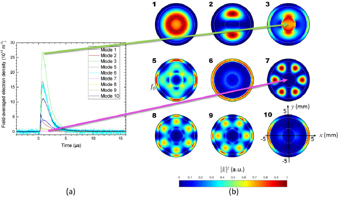
Figure 7. (a) Cavity-averaged values of  as a function of time before and after the gas was irradiated with a pulse of EUV radiation (at t = 0) obtained from different resonant modes and (b) simulated electric-field profiles through the whole cavity volume (including the ceramic and Teflon) for each of these modes. Background gas pressure was 10−4 mbar. The EUV beam was aligned axially at the centre of the cavity.
Download figure:
Standard image High-resolution imageIn the procedure we have developed, this 'raw' data is used to derive the absolutely calibrated maximum value of the electron density  , in a temporally resolved fashion. Note that—although only maximum values are presented in this section—our procedure is able to reconstruct absolutely calibrated and fully spatially resolved electron density profiles (as will be demonstrated in the next section). For reconstruction and absolute calibration, the field profiles of respectively five, six and seven different microwave resonant modes have been combined. For each set, figure 8 plots the results together with the upper and lower limit of the corresponding 95% confidence interval and the temporal evolution of the radial width σ of the calculated electron density distribution.
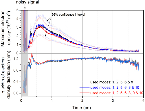
Figure 8. Top: maximum electron density  as a function of time after gas irradiation combining respectively five, six and seven different modes (see inset for the specific modes used). The greyed-out curves indicate the upper and lower limits of the corresponding 95% confidence interval. Bottom: temporal evolution of the radial width σ of the electron density distribution retrieved from the same data.
Download figure:
Standard image High-resolution imageFrom this figure, it can be concluded that—especially during the first 220 ns of the profiles shown—the signals contain too much noise to deliver valuable information. This noise is caused by EMC from the EUV source just before it emits the main in-band EUV radiation and is more dominant in our measurements than in those in other literature [14] because no spectral purity filter (SPF) has been used here (SPF normally blocks part of the EMC form the source). Between 220 ns and 380 ns, the general trend for the different sets of resonant modes used appears to be the same but the absolute values are not consistent. The reason for this is that timescales for plasma dynamics in this range are of the same order as the response time τ of the cavity used (roughly 100 ns, see table 1). Since τ is different for different resonant modes, it is not surprising that the  and σ curves diverge from one another when different sets of resonant modes are used to construct them. In this range, it is important to note that, although absolute values of the electron density and its spatial distribution width might not be very accurate, trends in temporal evolution can be made visible at sub-100 ns timescales. The reason for this is that MCRS reacts to trends even when the specific resonant modes are not yet fully loaded. Beyond 380 ns, the same results are produced when taking into account different sets of resonant modes. This indicates the reliability—in terms not only of temporal evolution, but also of absolute values—of the multi-mode MCRS approach we have developed.
4.2. Multi-mode MCRS: mapping electron dynamics at low-pressure EUV photon-induced plasmas
A zoomed-in picture of the curves reconstructed using modes 1, 2, 5, 6 and 8 is presented in figure 9 with—for clarity—independently measured [37] (but synchronized in time with the other data) out-of-band and in-band EUV-radiation intensity delivered by the same EUV source at the same position in the cavity.
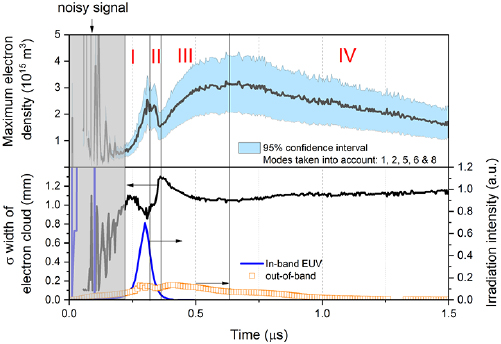
Figure 9. Top: maximum electron density  as a function of time using modes 1, 2, 5, 6 and 8, together with the corresponding 95% confidence interval. Bottom: temporal evolution of the radial width σ of the electron density distribution retrieved from the same data together with independently measured in-band EUV radiation and out-of-band radiation from the same xenon-pinch discharge source [37]. The time axes have been aligned with one another.
Download figure:
Standard image High-resolution imageIn order to discuss the plasma dynamics involved, the time evolution of the system has been divided in four different phases (denoted I–IV in figure 9). As already explained in the previous section, dynamic processes in phases III and IV are sufficiently slow, compared with the cavity response time τ, to deliver accurate and absolute results. Processes and time behaviour in phases I and II are of the same order as or faster than τ, meaning that although dynamics can be probed in relative sense using this method, absolute values may be less accurate.
As can be observed from figure 9, from approximately 220 ns onwards the measured signal-to-noise ratio is sufficient to obtain  and the radial width σ of the electron density profile as a function of time.
In phase I, the increase in  is directly related to the upcoming in-band EUV irradiation creating free electrons in the cavity by photoionization of the background gas. Assuming that the majority (~80%) of the gas present is N2, the majority of these electrons primarily have an energy (76.4 eV) equal to the difference between the photon energy (92 eV at 13.5 nm) and the ionization potential (15.6 eV for N2). Note that the electron-energy distribution function (EEDF) is highly non-Maxwellian shortly after the electrons have been produced. In this phase, σ is observed to decrease until the in-band EUV intensity has reached its maximum. At very short timescales (a few ns), the first electrons reach and charge the inner cavity wall while the created ions remain are still fixed in position due to their high inertia. This creates an elevated plasma potential and radially directed electric fields confining additional electrons and preventing them to be lost from the plasma. The observed contraction of the spatial electron distribution is explained by two processes. First, continued production of electrons on the axis of the cavity while its inner surface is already in quasi-equilibrium with the elevated plasma potential results in a spatial electron density distribution which is higher at the axis of the cavity. Second, electrons which have not been involved in charging the inner walls of the cavity start to oscillate through it without reaching the walls. Due to collisions with background molecules, these electrons lose part of their energy. This eventually confines the electron density distribution by the radial electric fields present. For initial electrons with energies in the order of ε = 76 eV, it can be estimated that the collision time of those with the mainly N2 background gas molecules is indeed in the order of 80-100 ns, as calculated with [45],
where v(ε) and  are the electron velocity and the electron-N2 collision cross-section respectively, and
  is the N2 density. At the same time, computing the inverse ion plasma frequency by
yields timescales of the same order (~80 ns). This indicates that, on the same timescales, ions start to move together with the electrons towards the walls, where they eventually recombine.
In phase II, the in-band EUV irradiation intensity has passed its maximum value and decreases as a function of time. Consequently, the production of free electrons also decreases while the loss rate due to plasma recombination at the wall continues. Overall,  tends to decline over time while the width of this distribution increases due to the expansion of the plasma.
In phase III, we observe a special behaviour which has not been seen before. Even though the main in-band EUV irradiation has now faded out, electrons continue to be produced. Since the width of the electron distribution decreases in this phase, these electrons must be produced or gathered along the cavity axis. Although the exact process is not yet fully understood, two processes may be responsible for this behaviour.
First, it is very likely that out-of-band radiation containing photons with energies higher than the ionization threshold of the background gas is responsible for significant photoionization even after the in-band EUV radiation has faded out. As can be seen from the orange curve in figure 9, the shape and timescales of the out-of-band emissions match the observed time evolution of the  profile. The fact that a considerable number of electrons is produced even though the out-of-band emission intensity is just a fraction of the in-band one is easily explained by the photoionization cross-section of N2, which is more than an order of magnitude higher just above the ionization energy threshold (2.5 × 10⁻²¹ m2 at 15.6 eV [46]) when compared with its value in the in-band regime (2.5 × 10⁻²² m2 at 92 eV [46]). Second, a significant number of the electrons produced by the in-band radiation (in phases I and II) remain confined in the positive plasma potential during this phase. Whereas the energy loss of 76 eV electrons is initially very fast (<100 ns [45]), electron energy-loss times in 1 Pa N2 just above ionization thresholds are computed by van de Ven [45] to be ~2 × 10² µs. Scaling linearly with gas density, this translates to roughly 2 µs for the pressures involved in the experiments reported here.
As during the second part of phase I, the creation of additional electrons on the axis of the cavity combined with cooling of the electron distribution narrows the width of that distribution.
In phase IV, production of electrons decreases while the plasma is transported towards the walls, where it decays due to wall recombination.
4.3. Multi-mode MCRS: application for beam power, profile and pointing stability monitor
Output parameters of the multi-mode MCRS measurements are the position ( ,
,  ) of the maximum
  of the electron density profile and its width σ(t). Once these have been derived from the measurements, absolutely calibrated electron density profiles can be retrieved for every time step. This means that, from an application point of view, the multi-mode MCRS diagnostic presented here can be used as a non-intrusive and in-line beam monitor for ionizing radiation. Parameters that can be derived from this method and used in, say, feedback loops in the source control are: beam power or energy per pulse, cross-sectional beam-intensity profile and pointing stability. This is all due to the fact that the initial electron density profile translates to the cross-sectional shape of the EUV beam and that the number of electrons created translates directly to the EUV pulse energy, i.e. the number of photons (with known photoionization cross-sections, gas purity and gas pressure). As shown by our measurements, the background gas pressure can be kept low (10−4 mbar, or even lower as long as the MCRS signal remains above the lower detection limit) while obtaining sufficient signal for the diagnostics to work.
5. Pulse energy
Traditional MCRS provided cavity-averaged and electric-field-weighted values of the electron density  . With the development of multi-mode MCRS, the measured electron density is corrected with the distribution of the electric-field component of the resonant mode used. This basically provides—with fixed-cavity geometry—a total number of electrons produced inside the cavity. Knowing the cross-section of the gas used and the instrumental configuration, sufficient data becomes available to determine the time-averaged power or the energy per pulse provided by the source. Of course, the equations used to translate the measured signal into pulse energy depend on the spectral purity filter used, the type of gas and its pressure, and should be determined according to the specific application situation.
6. Beam shape and position
As a demonstration, figure 11 shows the absolutely calibrated and spatially resolved electron density profiles for six different moments in time (denoted with red dashed lines in figure 10) along the x-axis and y-axis of the cavity. Here, we stress again that in the reconstruction procedure (section 2.2.1) a Gaussian profile shape has been used for the radial electron density distribution. This choice was made because in the current application of beam monitoring, one would be mainly interested in the situation at the moment of photoionization by the EUV beam (in which the radial photon density is distributed Gaussian as well). At longer time scales after EUV irradiation, a Bessel-like profile shape may represent plasma dynamics slightly better. Of course, different profile shapes can be used without any problem in the reconstruction method as well. As can be seen from the diagrams in figure 11, both the centre point ( ,
,  ) and the distribution width σ evolve over time and follow the different phases as explained in the previous section. Additional information that can be retrieved from the plots in figure 11 includes the fact that the EUV-induced plasma is generated (at t1 = 0.308 µs) slightly off the axis of the cavity (i.e. x0 = −1.57 mm, y0 = −0.76 mm). Furthermore, it can be concluded that—especially in the x-direction—the bulk of the plasma evolves over time in a certain direction. This could be explained by, for example, slight misalignment of the EUV beam with the axis of the cavity or by asymmetrical geometry of or close to the cavity. Another reason might be that the out-of-band EUV-radiation part of the beam is usually wider than its in-band EUV part.

Figure 10. Maximum electron density  as a function of time. The red dashed lines indicate the moments when spatially resolved electron density distributions have been reconstructed. These results are plotted in figure 11.
Download figure:
Standard image High-resolution image
Figure 11. Absolutely calibrated and spatially resolved electron density profiles for six different moments in time along the cavity x-axis (a) and y-axis (b).
Download figure:
Standard image High-resolution imageAs a direct cross-check for this application, the reconstructed  profile at the moment of maximum value of
  (i.e. at t1 = 0.632 µs) is compared with a fully independent measurement of the cross-sectional beam-intensity profile (see figure 12). This independent measurement is conducted using an EUV-light-sensitive foil placed at the position of the centre of the cavity and correlates well with the multi-mode MCRS measurements.
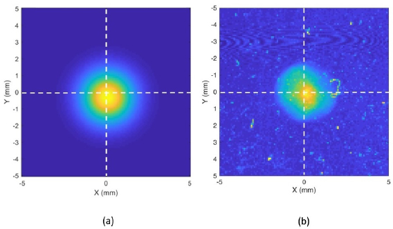
Figure 12. (a) Reconstructed ne profile at the maximum intensity of in-band EUV emission and (b) an independent measurement of the beam-intensity profile at the position of the cavity. Reproduced with permission from [47].
Download figure:
Standard image High-resolution image7. Conclusions
The following conclusions have been reached from the work presented in this article.
- (1)A novel non-invasive plasma diagnostic called multi-mode microwave cavity resonant spectroscopy (multi-mode MCRS) has been developed and introduced. This is based on traditional MCRS but enables the generation of absolutely calibrated data in a spatially resolved (100 µm resolution) fashion and corrected for the electric-field component of the resonant mode used. It should be noted that this is the first time a diagnostic method has been able to determine spatially resolved distributions of free electrons instantly, and also that its application is not limited to EUV-induced plasmas, as taken as a 'test case' here, but also extends to all types of plasmas with electron densities below roughly 1017 m−3.
- (2)The electron dynamics during the creation and decay of a highly transient plasma induced by irradiation of a gas at low pressure with a pulsed beam of EUV photons was monitored. Plasma creation and decay were found to match the time evolution of the in-band EUV irradiation, but significant additional production of free electrons was observed at much longer timescales. This behaviour was attributed to production of electrons by photoionization due to ionizing out-of-band radiation from the source and/or by electron-impact ionization by electrons initially created by in-band EUV irradiation.
- (3)The application potential of multi-mode MCRS in monitoring beam properties of ionizing radiation has been demonstrated. The measurements presented in this article show that multi-mode MCRS is able to monitor the pointing stability, cross-sectional intensity profiles and pulse energy of the utilized pulsed beam.
Acknowledgments
The authors acknowledge the financial support of the Dutch funding agency NWO (project number HTSM2015:14651) and of ASML. They are also grateful to the research department of ASML for providing measurement time on its EUV source and to Dr Marco Zangrando from Elettra Sincrotrone Trieste, Italy for fruitful discussions.
Appendix A. CST Microwave Studio simulations of E-field profiles
So-called eigenmode simulations of the electromagnetic resonances in our cavity were performed with CST Microwave Studio. A hexahedral mesh was used in conjunction with the Advanced Krylov Subspace solver. The model geometry is shown in figure A1 and has the same dimensions as the real cavity, though the geometry itself is somewhat simplified (no antenna and associated slots, solid metal housing instead of base plus screw lid). The metals are modelled as perfect electric conductors. The simulation bounding box snugly fits the outside of the cavity, except at the end faces where it extends 10 mm into the vacuum in both directions (z). The total mesh contains a little over 700 000 cells. The ceramic and Teflon were modelled with constant relative permittivities of 35.6 and 2.1 respectively, yielding good correlations between the simulated and measured resonance frequencies of the modes up to 4 GHz. The resulting vectorial electric-field amplitudes within the bounding box, of  and
and  (the mass centre of the ceramic is the origin), were interpolated onto a regular rectangular 3D grid with 100 µm spacing and exported for processing in Matlab.
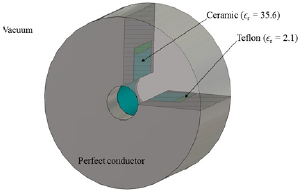
Figure A1. Cut-out of the axisymmetric simulation geometry of the cavity.
Download figure:
Standard image High-resolution imageAppendix B. Bead-scanning method
Inside the cavity enclosed by the dielectric material, i.e. the volume where the plasma is created, the electric-field component of each resonant mode is determined, spatially resolved, by using a 1.5 mm diameter BaTiO3 bead connected with superglue to an 80 µm thick nylon fishing line to disturb the mode structure locally. By scanning this local disturbance through the volume and monitoring the response of the cavity (in terms of a shift of Δf in the resonance frequency f0 of the mode under investigation) to it, using Slater's perturbation theory information about the local electric field  at the position of a spherical bead
  can be retrieved by means of the following equation [39]
This shows that  . In practice, in the bead-scanning method,
  is measured for each relevant resonant mode and for fixed positions
  of the bead. During the calibration measurements, the bead was directed through the volume by an automated XYZ translation stage with spatial resolutions of 250 µm in both the X and Y planes (see figure B1) and of 500 µm in the Z plane. The holes in the top and bottom lids of the cavity—serving as the entrance and exit for the EUV radiation—might be responsible for 'leakage' of part of the mode structure outside the cavity. To be able to take this effect into account and to correct for it during absolute calibration, the electric field distribution is scanned in the Z direction from 2.5 mm below the bottom lid of the cavity up to 2.5 mm above its top lid. In all, a spatially resolved measurement of the electric field profile for each single resonant mode consists of 36 941 datapoints.

Figure B1. Datapoints, i.e. bead locations, in the XY plane taken into account in the bead-scanning method. The arrows indicate the trajectory the bead followed over time. For each relevant resonant mode, the cavity response Δf/f0 has been measured for each of these datapoints; this procedure has been repeated for 41 Z positions along the axis of the cavity.
Download figure:
Standard image High-resolution imageAppendix C. Additional results from bead-scanning and CST microwave studio simulations

Figure C1. Electric-field profiles obtained experimentally using the bead-scanning method (left column) and simulated using the CST Microwave Studio package (right column) for modes 5, 6, 8, 9 and 10.
Download figure:
Standard image High-resolution image