
Abstract
This review is devoted to the study of ultrafast laser ablation of solids and liquids. The ablation of condensed matter under exposure to subpicosecond laser pulses has a number of peculiar properties which distinguish this process from ablation induced by nanosecond and longer laser pulses. The process of ultrafast ablation includes light absorption by electrons in the skin layer, energy transfer from the skin layer to target interior by nonlinear electronic heat conduction, relaxation of the electron and ion temperatures, ultrafast melting, hydrodynamic expansion of heated matter accompanied by the formation of metastable states and subsequent formation of breaks in condensed matter. In case of ultrashort laser excitation, these processes are temporally separated and can thus be studied separately. As for energy absorption, we consider peculiarities of the case of metal irradiation in contrast to dielectrics and semiconductors. We discuss the energy dissipation processes of electronic thermal wave and lattice heating. Different types of phase transitions after ultrashort laser pulse irradiation as melting, vaporization or transitions to warm dense matter are discussed. Also nonthermal phase transitions, directly caused by the electronic excitation before considerable lattice heating, are considered. The final material removal occurs from the physical point of view as expansion of heated matter; here we discuss approaches of hydrodynamics, as well as molecular dynamic simulations directly following the atomic movements. Hybrid approaches tracing the dynamics of excited electrons, energy dissipation and structural dynamics in a combined simulation are reviewed as well.
Export citation and abstract BibTeX RIS

Original content from this work may be used under the terms of the Creative Commons Attribution 3.0 licence. Any further distribution of this work must maintain attribution to the author(s) and the title of the work, journal citation and DOI.
1. Introduction
Ultrafast laser ablation, that is the removal of matter from solid surfaces or bulk irradiated with an ultrashort laser pulse, is of great fundamental and practical interest motivating experimental as well as theoretical research [1–4]. Experiments have shown that with ultrashort irradiation a better controllability and precision in material modification can be achieved as compared to longer pulses [2, 5]. Monitoring transient behavior, femtosecond ablation has lead to such new observations as e.g. Newton rings in pump–probe experiments [6]. From the theoretical point of view the ultrashort time of excitation allows the separation of the involved processes as excitation, melting, and material removal. Moreover, subpicosecond laser ablation opens interesting opportunities for the investigation of optical and thermodynamic properties of matter with an electron temperature noticeably higher than the temperature of the crystal lattice.
The energy of the irradiating laser is mainly absorbed by the electrons of the solid. The laser therefore initiates a transient nonequilibrium of the electron gas with the lattice, which was first pointed out in this context in [7, 8]. During a short period of a few picoseconds or less, the lattice remains at its considerably lower temperature. The kinetics of electron–lattice relaxation were considered in [9, 10]. It was shown that the energy exchange between electrons and the lattice can be described by the equations

where  and
and  are the electron and lattice temperatures and specific heats, respectively, and α is the energy exchange rate between the two subsystems.
Another process that affects the temperatures of electrons and ions is the energy transport from hot surface layer to the bulk of the material by thermal conduction. In metals the energy transport is normally due to electron heat conduction. In special cases, however, lattice heat conduction should be taken into account as well. Inserting classical thermal conduction terms into equation (1), we arrive at a set of equations for electron and lattice temperatures

where Q is the energy released in the electron subsystem due to laser radiation absorption, and  and
and  are thermal conductivities of the electron and phonon subsystems respectively.
The two-temperature model (TTM) in equations (2) and (3) allows for theoretical predictions for instance on melting thresholds or heating rates and has been widely applied to explain experimental observations in laser-irradiated metals [5, 11–14]. In spite of its widespread implementation, some limiting cases of the applicability of the TTM should be mentioned here. First, on the femtosecond timescale, which is the timescale on which electron–electron collisions typically occur, it may be questionable to speak about a temperature of the electronic system. The energy may be inherent in the electron gas in a nonequilibrium manner, while the concept of temperature is generally restricted to equilibrium energy distributions. Second, the TTM is derived under the assumption that electron and phonon energy transport is described by the classical Fourier law. This approach is valid as long as the characteristic space and time scales of the temperature field are much greater than, respectively, mean free path and relaxation time of the energy carriers. And third, the material parameters of the lattice may change during the time of calculation in case phase transitions are involved.
In this work, we review results obtained with help of the TTM, as well as the development and the resulting insights of alternative and amendatory methods. In this rapidly developing field, we aim to bring results and single aspects of our previous approaches in relation to studies of various other authors. The modelling of ultrafast laser ablation is a complex task involving a large variety of timescales requiring different methods or multiscale approaches. The response of the material on initial excitation depends on the type and peculiarities of the material as well as on the laser parameters like photon energy and intensity. Here, we restrict ourselves to excitation with visible light in the intensity range close to ablation threshold. Moreover, when spatial scales are involved, we focus on one-dimensional descriptions. They are a reasonable approximation for cases when the laser spot size is much larger than the depth affected by the irradiation, which is typical for ultrashort-pulse laser melting and ablation experiments. Regarding different materials, we distinguish in a generalised manner between absorbing materials with a degenerate free electron gas, i.e. metals, and transmitting (or 'band gap-') solids such as dielectrics and, to some extent, semiconductors. For both latter types of solids, the excitation of a certain density of free electrons plays an important role for the further development of the irradiated material.
An overview of typical involved phenomena in the considered parameter range is given in figure 1 which shows pathways of the material from excitation to ablation, depending on the relevant timescale and intensity ranges. Excitation of the solid takes place during the laser pulse. Depending on excitation strength, melting occurs roughly on a picosecond timescale. In semiconductors and dielectrics irradiated with high laser intensities, the loss of crystalline order is possible within less than one picosecond. The state of the material after irradiation depends strongly on the type of material and on laser properties such as intensity and wavelength. Expansion and ablation of the laser-excited material lasts up to the nanosecond regime. For ultrashort laser irradiation, these processes separate and can thus be considered to some extend sequentially. The range of intensities in figure 1 reaches from about 1010 W cm−2 to above 1014 W cm−2. At these intensities, a large variety of phase transitions can be observed. In this work we refer to this range as 'moderate to high intensities'. At moderate intensities, melting is induced in metals, while with higher intensities dielectrics too can be excited and even transferred directly to the plasma state. Note that some discussions are also valid for 'low intensities', which are considered to be intensities below the melting threshold.
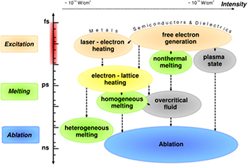
Figure 1. Typical timescales and intensity ranges of several phenomena and processes occurring during and after irradiation of a solid with an ultrashort laser pulse of about 100 fs duration. Excitation takes place in the range of femtoseconds (duration of the laser pulse). The timescale of melting may vary for different processes and lies roughly in the picosecond regime. Material removal, i.e. ablation, lasts up to the nanosecond regime. Figure adapted from [16] with permission of Springer.
Download figure:
Standard image High-resolution imageThe paper is structured according to the timescales of the involved processes. In the next section, we discuss models describing the absorption of energy on ultrashort timescales in different types of materials. Section 3 is devoted to the electron–lattice energy transfer. In section 4, we report on the thermal conduction to the bulk of material. The models and descriptions in these initial sections are valid for the initial stage of laser ablation, when the material is still of solid state density. After that we review different approaches to study structural dynamics of the heated material. While section 5 refers to phase transitions at solid density (in particular melting), the subsequent sections 6 and 7 consider expansion of the material, described with hydrodynamic and molecular dynamic methods, respectively. In section 8, we review hybrid approaches where electronic and atomic behavior is studied in combined simulations. Section 9 closes the review with summary and conclusions.
2. Absorption of ultrashort pulses
When a laser irradiates the surface of a solid, the laser energy may be absorbed. In metals the optical absorption is usually dominated by free carrier absorption, i.e. electrons in the conduction band absorb photons and gain higher energy. In semiconductors, electrons are excited from the occupied valence bands to empty conduction bands, provided that the photon energy exceeds the band gap. In dielectrics with band gaps larger than the photon energy, nonlinear optical effects like multiphoton transitions are necessary to promote electrons from the valence band to the conduction band. In all these cases, the timescale of the energy deposition is determined by the laser pulse duration.
In the following, we discuss simplified descriptions for laser absorption, capable to serve as initial conditions for further modelling of the induced processes up to final ablation. Since the characteristics and proper descriptions of absorption depend mainly on the band gap of the irradiated material, we distinguish in sections 2.1–2.3 between metals with free electrons in the conduction band, semiconductors with a band gap in the range of the photon energy of the laser and dielectrics with larger band gaps. In section 2.4, we show kinetic views on how the laser excitation disturbs the electronic system to a nonequilibrium distribution and present results on its thermalisation.
2.1. Metals
Free electrons are present in the conduction band of a metal. Electrons below the Fermi edge can absorb photons and end at energies above the Fermi edge. The average energy increase due to intraband absorption can be described in terms of Drude's approach [17]. In this picture, electrons move in the electric field (here the field of the laser light, alternating with frequency  ) and collisions, occurring with a frequency
  , hamper the movement of the electrons. This leads to a dielectric function of

where  is the dielectric constant of the unperturbed material and
  the plasma frequency, determined by the density of the free electrons ne and their effective mass
  . Note that the choice of the collision frequency
  varies in literature. Matthiesen's rule can be applied to include several types of collisions in this so-called Drude frequency. This frequency
  is roughly connected with the transport time τtr, appearing in equations (21) and (28); however, when interested in absorption, collisions among free electrons of the same effective mass should not be included since the collective momentum of this electronic system is not changed in such collision. Often a constant
  is assumed [18–21] which lies in the range of
  , corresponding to a collision time in the femtosecond range. However,
  is likely to depend on material parameters which may change during irradiation. For instance, the electron–phonon collision time
  depends on the lattice temperature Ti. For further increasing temperature, the limit of hot plasma may be reached. Here, the collision frequency is given by Spitzer's formula [22], where the collision frequency decreases with increasing electron temperature. A transition from the initially cold metal to a hot plasma was discussed in [23]. Moreover, since the Drude model also applies roughly for free electrons in semiconductors and dielectrics, the dependence of
  on the electron density ne may become crucial [24]. Generally, it should be noted that vD is rather a phenomenological than a microscopical parameter [26].
The square root of the dielectric function (4) equals the complex refraction index  ,
,

where n is responsible for the refraction of light and k determines the attenuation of an electromagnetic wave in material. The reflectivity R and the free carrier absorption coefficient afca follow as
with c denoting the velocity of light in vacuum. In weakly excited metals, linear absorption can be assumed, where the absorbed energy per unit volume and time is proportional to the photon flux, i.e. the intensity I. This results in an exponential decay of laser energy in the material, which is described by the Lambert–Beer extinction law,

where Ilas is the laser intensity irradiating the material, IS = Ilas (1 – R) is the resulting intensity at the surface after reflection, and  the absorption coefficient. The source term in equation (2) is then given by

Note that interband absorption mechanisms may also play a role in metals. In polyvalent materials like aluminum, nearly-parallel bands lead to an increased absorption at certain laser frequencies [25–28]. An even more complicated picture appears for noble metals, where the d band lies energetically in the s band of free electrons. Here, d electrons may be excited into the s band above the Fermi level with sufficiently high photon energies. Such transitions cannot be described in the frame of the Drude model and more sophisticated approaches have to be applied [29].
In practice, the strength of absorption, i.e. the parameter  in equations (7) and (8) is often taken from tabulated data [30], in particular when the behavior of a real, non-idealised material shall be modelled. Note, however, that even in metals this parameter may change considerably under strong electronic excitation [28, 29, 31].
Experimental works have shown an effective penetration of laser energy considerably larger than the optical light penetration: time-resolved front pump–rear probe experiments revealed that a thin layer of gold is heated homogeneously up to a thickness of approximately 100 nm [14]. This effect was attributed to ballistically moving electrons, heating a layer with a thickness of their free path  . The authors proposed to consider this effect in the TTM, applying in the source term (8) an effective penetration depth

In [32] this expression was incorporated into the TTM for copper, silver and tungsten. The numerical results on ablation depths were compared with experimental observations. The authors found a ballistic depth of about 15 nm for copper and 50 nm for silver (and none for tungsten). The inclusion of an effective absorption coefficient according to equation (9) has been found to be important only for fluences close to ablation threshold. This finding is consistent with an estimation connecting the ballistic range with the time of free flight of the electrons (entering transport, see equation (28)), leading to a decreasing  for increasing temperatures [33]. Generally, the concept of ballistic electrons is not directly compatible with a temperature-based description. Therefore, expression (9) seems to be practical—however, it is questionable in the kinetic view.
2.2. Semiconductors
The description of laser light absorption in semiconductors has to take into account changes in the density of free electrons in the conduction band of the material. Since conduction band and valence band are separated by a bandgap which is typically in the range of the photon energy of visible light, the generation of an electron–hole plasma upon irradiation plays a crucial role [18]. The absorption of laser energy by free electrons in the conduction band can be described with the Drude formalism as sketched in the previous section. Also absorption by holes can be described in this framework [18]. Note that the plasma frequency  in equation (4) depends on the density ne of free carriers (i.e. electrons and holes).
The attenuation of the laser intensity I in the material is strongly connected with the excitation of the free electron density ne (or, equivalently, the density of the electron–hole plasma  ). In many cases, single photon absorption across the band gap has to be considered, as well as two photon absorption. For instance in silicon irradiated with visible light, two photon absorption may be a direct transition while single photon absorption is indirect and thus accompanied by a momentum change. Depending on photon energy, three photon absorption may also be of considerable importance, but is neglected in the formula presented in the following. The attenuation of laser intensity by single- and two photon absorption as well as free carrier absorption is given by [18, 24, 34, 35]

where a0 denotes the single photon absorption coefficient and b0 the two-photon absorption coefficient. Free-carrier absorption can be identified with Drude absorption, compare equations (4) to (6). However, note that the dielectric function  may consist of more terms than equation (4) for excited semiconductors [18, 24]. In case two-photon absorption can be neglected (i.e. b0 is small in equation (10)), the Lambert–Beer extinction law (7) applies with
  . Note that
  may strongly change during irradiation [24].
The increase of free electron density due to these direct laser-induced excitation processes is given by [18]
For the complete description of the transient free electron density in laser-excited semiconductors, additional excitation and recombination processes have to be included. In [34], electron impact ionisation and Auger recombination have entered the balance, thus
where  denotes the impact ionisation coefficient and
  the coefficient of three-body Auger recombination. When particle transport comes into play, further processes influence the transient local density of the electron–hole plasma [24, 34, 35]. The resulting modified description of the energy density similar to the TTM, equations (2) and (3), will be discussed in section 4.4. Note that the description of the optical parameters according to equation (6) leads to a very good comparability of calculated melting thresholds with experimental values for a large range of pulse durations [24], once a density- and temperature dependent Drude collision frequency is taken into account.
A modified description of free electron density evolution in semiconductors tracing also nonequilibrium electron distributions has been presented in [36]. It is based on the multiple rate equation for dielectrics [37, 38], which will be described in the following section. In the extended multiple rate equation [36], Auger recombination processes and electron–phonon coupling have been implemented additionally. The results have shown good agreement with experimental findings [18].
Strong excitation of semiconductors may considerably change their optical properties. In [39–41], it was reported that GaAs turns into a metallic state after irradiation with a femtosecond laser pulse. The underlying ultrafast phase transitions are discussed in section 5.2 of this review, with a focus on the loss of crystalline order. Note that the accompanying change of the optical properties may influence the energy input for sufficiently long laser irradiation.
2.3. Dielectrics
In wide-band gap dielectrics, absorption of visible light is possible only when high intensities are applied, allowing for nonlinear optical processes. The studies of laser-irradiation of dielectrics in the context of material ablation focus mainly on the time-resolved description of the free electron density. The common argumentation includes that for increasing electron density the real part of the dielectric function (4) may vanish and further become negative, leading to an imaginary refractive index (5) accompanied by a strong metallic-like absorption, compare section 2.1. The critical density ncrit of this transition can be calculated under the assumption of  to
to
Figure 2 shows the dependence of optical parameters on the free electron density ne [42]. A laser with a wavelength of  (corresponding to a frequency of
  ) and intensity
  has been assumed to irradiate on a quartz-like material with
  . The Drude collision frequency was taken as
  and the effective mass me was assumed to equal the free electron mass. Note that in this case the assumption
  is not fulfilled and the considerable increase of absorption, given by
  , is a smooth function rather than resembling a threshold behaviour.
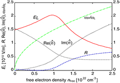
Figure 2. Change of optical parameters in dependence on free electron density ne, here denoted as nfree. The reflectivity, real and imaginary part of the complex refraction index  , as well as the changing electrical field amplitude EL inside the material are shown. A quartz-like material with
  and a laser with a wavelength of 500 nm and an intensity of
  was assumed. Figure reproduced from [42] with permission of Springer.
Download figure:
Standard image High-resolution imageNote that besides the free-electron response following from its dielectric function (4) other interesting optical phenomena occur in laser-irradiated dielectrics. For instance, the light attenuation (as described for semiconductors with equation (10)) includes self-focussing and defocussing, which are nonlinear optical processes becoming important for high intensities and high free electron densities [3, 43]. Propagation of the laser in certain parameter ranges may therefore result in long-distance filamentation, observed in various materials [44–47].
The increase of free electron density in the initially empty conduction band of a dielectric is triggered first by photoionisation from lower bands. During multiphoton ionisation, many photons are absorbed in one step. For very high intensities this process transfers to tunnel ionisation [48]. The transition is characterised by the so-called Keldysh parameter  , where mred is the reduced mass of electrons and holes,
  the band gap and
  the electric laser field amplitude. The Keldysh parameter is essentially determined by the ratio of the band gap energy
  to the ponderomotive energy of the electron oscillating in the electric laser field,
  . For a large band gap and small electrical field amplitude (i.e. small ponderomotive energy) many photons have to be absorbed. This multiphoton regime is characterised by
  . When the ponderomotive energy exceeds by far the band gap,
  , the latter becomes unimportant and electrons can appear in the conduction band. This process may be interpreted as a tunnelling process across potentials bent by the electric laser field. The ionisation rate for the process of photoionisation in strong laser fields was calculated by Keldysh in [48]. For various material and laser parameters, it is plotted for instance in [4, 43, 49]. Approximative expressions describe either the multiphoton- or the tunnelling regime [48]. In [49], a simplified complete description as a weighted transition between both regimes was proposed. Modified derivations have been proposed in [50, 51]. Experimentally determined values of the multiphoton ionisation cross sections are also available [52, 53].
When electrons are present in the conduction band of the dielectric, they may enable further electrons to overcome the band gap [54, 55]. This is the case for free electrons with a high energy above a certain critical energy  , which is on the order of the band gap energy [49]. The corresponding impact ionisation rate may be assumed to directly depend on the free electron density, compare also equation (12). Considering photoionisation with a rate
  and impact ionisation with a probability
  , the increase of free electron density in dielectrics is given by the addition of both contributions [55, 56],
However, experimental studies applying equation (14) have led to contradictory results [19, 52, 53, 56, 57]. Moreover, theoretical investigations state fundamental doubts as to whether this standard rate equation is applicable in general in the subpicosecond time regime [49, 58, 59]. One basic assumption of equation (14) is that impact ionisation depends directly on the total density of the free electrons. However, since impact ionisation needs a certain critical energy of the ionizing electron, this process also depends on the energy of a particular electron in the conduction band. While photoionisation generates electrons with low kinetic energy in the conduction band, impact ionisation requires electrons of high kinetic energy. This additional energy is absorbed from the laser light by intraband absorption. If this absorption process takes time comparable to the laser pulse duration, it is obvious that equation (14) is oversimplified. Such discrepancy will be reflected in a non-stationary shape of the free electron energy distribution. Examples of such distributions on ultrashort timescales, obtained with kinetic approaches [49, 60], are shown in the following section 2.4. Note that in [61] a description similar to equation (14) was proposed, where the intensity-dependence of the avalanche parameter was discussed in more detail. The idea of the authors is that impact ionization may be assisted by further photon absorption. For sufficiently high intensities such a process seems to be likely; however, its inclusion into the parameter  still does not capture the time dependence of the electrons' energy increase. Another qualitative way to include such time dependence into the description of impact ionization has been proposed in [3]. It is based on an empirical delay time and applies the electron density at earlier times to calculate the current rate of density increase by impact ionization.
In a microscopic picture, the energy distribution of the electrons has to be traced. The possibility to keep track of this distribution without applying a complex full kinetic approach has been introduced with the multiple rate equation (MRE) in [37, 38]. Here, the rate of intraband absorption W1pt and thus the time of energy increase by one photon energy has been included in a description maintaining the conceptual simplicity of the rate equation (14). The MRE introduces virtual intermediate levels of energy in the conduction band and counts the density of electrons at these levels. Photoionisation provides electrons at the lowest energy, increasing the density n0, while the density of electrons with energies above critical energy for impact ionisation  is denoted as nk. The number of virtual levels k is given by the integer above
  . The multiple rate equation then reads

Here,  denotes the pure probability of impact ionisation in case an electron with energy
  is present. The absorption probability W1pt depends on the laser electric field amplitude EL. The inclusion of a possible dependence of
  on the electrons' energy
  was discussed in [38]. The free electron absorption probability W1pt can be roughly described with the Drude model, compare equations (4)–(6). Note again that the choice of the collision frequency
  is crucial for quantitative comparisons [24], and that different expressions and dependencies can be found in literature [18–21, 23, 24, 28].
Summing up the MRE, we obtain the rate of increase of the total free electron density ne, which is given by
On timescales larger than the timescale of the intraband absorption process, the shape of the electron distribution does not change significantly and the fraction of high-energy electrons  is temporally constant. Then, equation (16) reduces to the standard rate equation (14) with
  . For the non-stationary case, the fraction of high-energy electrons changes with time and the difference in the last term of equation (16) as compared to equation (14) is substantial. The transition from the non-stationary regime on ultrashort timescales to the asymptotic avalanche regime for longer timescales was calculated in [38]. In figure 3, it is marked for constant laser intensity I of pulse duration
  and photon energy
  as the line
  in the
  plane. The intensity refers to the intensity inside the material. Material parameters taken from SiO2 have been applied [38]. The line tMRE separates the parameter region of ultrashort irradiation where multiphoton ionisation dominates from that for longer pulses, where the collisional avalanche dominates the free electron generation.

Figure 3. Percentiles of the fraction of impact ionised electrons to the total free electron density in the plane of intensity (inside the material) and pulse duration (of constant intensity). Regions of dominating ionisation processes are shaded. They are separated by the transition time tMRE, which is a function of intensity inside the material and denotes the transition from the ultrashort pulse regime of non-stationary shape of electron distribution described with equations (15) to the longer regime, where equation (14) is applicable. Here, material parameters from SiO2 and a laser with a wavelength of 500 nm have been assumed. Reprinted figure with permission from [38]. Copyright (2006) by the American Physical Society.
Download figure:
Standard image High-resolution imageSeveral improvements and applications of the MRE (15) have been published since its introduction. It has successfully been applied to interpret experimental observations on laser damage and ablation with shaped laser pulses [62, 63]. An intensive discussion of the model was published by Christensen and Balling in [64]. In this work, energy conservation in the process of impact ionisation has been improved, the changing optical parameters during irradiation have been included and a depth-dependent analysis of the dielectric breakdown and ablation threshold has been performed. Also the limitations of the model in direct comparison with experiments have been discussed. For instance, the inclusion of defects would open the way to the description of more realistic material. For several applications also multishot experiments would be of interest. Other refinements mentioned in [64] as being necessary have meanwhile been performed, in particular the inclusion of fast recombination processes [42] as well as of nonlinear light propagation [43, 65] and relaxation processes [36, 43]. Note that when considering longer timescales up to the picosecond regime, recombination processes are of increasing importance. Particularly in SiO2, self-trapped excitons (STE) lead to a decrease of the free electron density on a timescale of only 150 fs [19, 66, 67]. Such recombination processes can be included in the rate equation with an additional term  , where
  is the density of free electrons (or of the virtual level in the MRE) and
  is the characteristic recombination time [42, 44, 68, 69].
It is important to note that apart from the large amount of publications considering the free electron density as the crucial parameter for laser damage of dielectrics, finally the absorbed energy is responsible for the damage of the material. Both thresholds are connected [70, 71], however, situations may occur where ne exceeds ncrit at the end of the pulse duration and no damage will be observed [60]. In [72] two criteria have been applied to calculated ablation depths, i.e. a criterion of electron density as well as of energy density. Both yield indistinguishable results for a broad range of incident fluences. In [72] it was shown that a model based on the MRE (15) is capable to reproduce all experimentally obtained quantities like change of phase shift, absorption, reflectivity and final depth of the ablation crater with one single set of model parameters.
2.4. Strongly excited electron distributions
As indicated in the previous section, the energy distribution of laser-excited electrons may determine the appropriate description of the absorption. It may also determine further energy dissipation processes like electron–phonon coupling and transport. The description in terms of a temperature, like in equation (2), might not be justified on ultrashort timescales, where strong nonequilibrium distributions can occur. The knowledge of the particular distribution may also be relevant for the interpretation of experimental data [73], especially on ultrashort timescales, where equilibrium distributions should not be assumed from the first. In this section, we show some examples of nonequilibrium distributions, review their influence on measurable quantities and the timescales of their thermalisation.
Kinetic approaches like the Boltzmann equation or asymptotic trajectory Monte Carlo simulations trace the electronic distribution function after ultrafast excitation in detail [49, 60, 73–77]. Here, the collision probability at each electron's energy enters the approach and no assumption on the energy distribution has to be made. Kinetic approaches are therefore applicable for the description of absorption and relaxation processes far from thermodynamic equilibrium, when no temperature can be defined. Figure 4 shows the energy distribution of electrons in the conduction band of a SiO2-like material during irradiation with a laser pulse of constant intensity. Details of the calculation are given in [49]. It can be seen that after a few tens of femtoseconds a smooth shape of the distribution is reached. This coincides with the calculations in [60] finding thermalisation times for electron distributions in dielectrics in the range of several tens of femtoseconds. Note that the thermalisation time reflects the smoothing of the distribution function towards a Fermi distribution (or, for sufficiently low densities, towards a Maxwell–Boltzmann distribution), whereas the transition time in figure 3 refers to the influence of two different ionisation processes, increasing the amount of electrons in this distribution. Ionisation and thermalisation are independent processes; for the given intensity in figure 4 the transition time is larger than the thermalisation time.

Figure 4. Energy distribution of laser-excited electrons in the conduction band of a dielectric with material parameters of SiO2. A constant intensity inside the material is assumed. The time after beginning of irradiation is indicated at each curve. The curves show the initial peak-like excitation due to multiphoton processes and subsequent intraband absorption as well as the thermalisation to smoother distributions on longer timescales. Reprinted from [71], Copyright (2012), with permission from SPIE.
Download figure:
Standard image High-resolution imageIn [78], the excitation and relaxation of different metals have been studied with help of Boltzmann collision integrals. Details of the density of states have been implemented in the calculation through an effective one-band model; they are reflected in the excited electron distributions [78]. The entropy of the excited distribution has been monitored after excitation. It increases to an asymptotic maximum value; the timescale of this increase can be identified with the thermalisation time  . Figure 5 shows the results for aluminum, gold and nickel. For nickel two curves are shown, which refer to two calculations with different screening parameters. The screening of the Coulomb potential by free electrons is important for the collision probability and thus the interaction strength of electrons with each other. The Coulomb potential decreases exponentially with a characteristic length
  . The so-called screening parameter κ can be directly calculated from the nonequilibrium energy distribution [79, 80]. For a thermalised distribution, i.e. in metals a Fermi distribution, the screening is known as Thomas–Fermi-screening, here denoted by the parameter
  . Figure 5 shows that the nonequilibrium screening remarkably increases the resulting thermalisation time. The influence of the screening length on
  is roughly a fourth power law, as the inset of the figure shows [78].

Figure 5. Entropy increase for laser-excited nonequilibrium distributions in different metals. The characteristic timescale of the increase can be identified with the thermalisation time  , here denoted as τ. The absorbed fluence is
  . The inset shows the dependence of the thermalisation time on the screening parameter κ for nickel. Here, β denotes a prefactor:
  . Reprinted figure with permission from [78]. Copyright (2013) by the American Physical Society.
Download figure:
Standard image High-resolution imageFor thermalised distributions, the electrons can be described in terms of temperature-based equations like (2). For strongly disturbed electron distributions such temperature  is not defined from the first. Only when the electrons thermalise to a new equilibrium distribution, the description in terms of an electronic temperature is justified.
However, kinetic descriptions as mentioned in this section are feasible only when spatial transport can be neglected. This is the case for homogeneously heated thin films or if only timescales below the picosecond regime are relevant. Since thermalisation is fast for high-energy excitation (below 100 fs for the considered cases, see figure 5), it is reasonable to assume that the TTM, equations (2) and (3), is applicable to describe ultrafast laser ablation. In case the nonequilibrium of the electron system leads to modifications of the energy absorption or dissipation processes, they may often be included in material parameters. Examples are, for instance, the modified absorption coefficient, equation (9), to capture ballistic transport, or a time-dependent electron–phonon coupling strength, which will be discussed in more detail in section 3.3.
3. Electron–phonon relaxation
After heating of the electronic system of the irradiated material, as has been described in the previous section, the electrons and phonons are out of thermodynamic equilibrium. Thermalisation of the electrons leads to a new Fermi distribution of elevated temperature, while relaxation of the electrons with the lattice leads to a joint temperature of electrons and phonons. Figure 6 sketches a possible timeline for these processes [81].
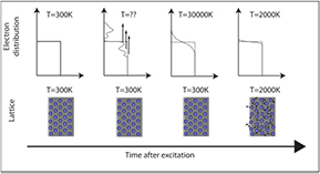
Figure 6. Sketch of the early excitation and relaxation processes in laser-irradiated metal. First, the electronic system is excited to a nonequilibrium distribution. Thermalisation to a new Fermi distribution of elevated temperature is sketched here before relaxation with the lattice to a joint temperature. Figure taken from [81], by courtesy of Peter Balling, Aarhus, Denmark.
Download figure:
Standard image High-resolution imageThermalisation is driven by electron–electron collisions, which occur on a timescale of femtoseconds. In contrast, relaxation with the initially cold lattice is determined by electron–phonon collisions. It should be noted that also electron–phonon collisions have a characteristic timescale of a few femtoseconds only. However, while such collisions lead to a large transfer of momentum, inducing a fast momentum relaxation of the electronic subsystem, the energy transfer is small. This is due to the small energy of a phonon emitted in such a collision ( is in the meV range) in comparison with the electronic energy (being in the eV range). In the classical view, a light electron collides with a heavy ion, leading to a large change of the electron's momentum, while the energy transfer is negligible due to the mass ratio of
  .
.
The energy relaxation time due to electron–phonon collisions is therefore about three orders of magnitude larger than the momentum relaxation time, thus in the range of picoseconds. More precisely it is the temperature relaxation which occurs on this timescale, since the nonequilibrium of temperatures is the driving force of energy exchange between electrons and phonons.
For thin metal films such temperature relaxation leads to a linear decrease of the electronic temperature, as will be described in the following section, section 3.1. The electron–phonon coupling strength itself depends on the properties of the conduction band electrons and, in particular in dielectrics and semiconductors, on their density. Approaches to determine the electron–phonon coupling parameter in metals, entering the TTM, equations (2) and (3), and an estimation for the coupling strength in semiconductors and dielectrics are presented in section 3.2. Finally, we mention effects of nonequilibrium and high excitation strengths and discuss possible consequences for the description in the frame of TTM-like models in section 3.3.
3.1. Temperature relaxation in thin metal films
If a thin film is irradiated with an ultrashort laser pulse, the energy is distributed by ballistic electrons on a femtosecond timescale and the film is homogeneously heated [14]. In this case thermal conduction can be neglected and the equation of heat exchange, equation (1), can be applied. Here, we assume that thermalisation is a fast process and the electronic system can be described by a temperature Te. It follows from equation (1) that the characteristic time of electron gas cooling due to energy exchange with the lattice is  , and the characteristic time of lattice heating is
  . The value of
  depends on electron temperature and ranges typically from 0.01 to 1 ps. Both characteristic times apply for the case that the temperature of the other subsystem is fixed. In case of electron cooling in laser-irradiated metals, it is
  and the assumption of a constant lattice temperature is reasonable as long as
  . If no further energy input is assumed and for
  and constant parameters ce, ci and α, equation (1) leads to a characteristic relaxation time of the temperature equilibration of [82]
Since usually  this time reduces to
  .
.
Assuming that the lattice temperature is initially equal to room temperature  while the initial electron temperature Te,init is much larger, the solution of equation (1) reads

where  is the joint asymptotic temperature of both systems. Here,
 and
and  [83]. The exponential function has thus a much higher influence on the electron cooling, while the change of lattice temperature remains small. For times ∼
 , the neglection of the change in lattice temperature is thus a reasonable approximation. With the heat capacity of a Fermi distributed electron gas given as
  , we end at
with the simple solution  We thus expect a linear temperature decrease in case the TTM is valid and γ and α are constants. This relation was utilised for the interpretation of ultrafast reflectivity measurements on laser-irradiated gold films of variable thickness in [14].
3.2. Expressions for the electron–phonon coupling strength
The first attempts to determine the relaxation between electrons and the crystalline lattice has been published by Kaganov, Lifshitz and Tanatarov in the context of the excitation of metals under ion impact [9]. Its relevance for ultrafast laser excitation was later pointed out by Anisimov et al in [7, 8]. Here, the energy exchange was described by equation (1). The creation of phonons by high-energy electrons was explained to correspond to the classical picture of Cherenkov radiation, emitted by a supersonic electron moving in the crystal. The integration over the probability of this process yields the electron–phonon coupling parameter α entering equation (1), for temperatures  and both temperatures much greater than the Debye temperature,
This expression contains the sound velocity in the material  and a characteristic time
  , which is the time of free flight of electrons (occurring in transport equations, e.g.
  in equation (28)) under the conditions of equal temperatures. For sufficiently low excitation strengths, in metals
  and thus the electron–phonon coupling parameter can be assumed as constant.
Allen [10] applies a more general expression based on Boltzmann collision integrals. His approach is valid for metals with arbitrary density of states, thus not bound to the assumption of free electrons. He connects the electron–phonon coupling parameter to the Eliashberg spectral function for electron–phonon coupling, commonly applied in the theory of superconductivity [10, 15]. The derivation of a coupling parameter near room temperature yields
The moment of the spectral function,  , can be obtained experimentally [15, 84]; the parameter λ is known in the theory of superconductivity as the electron–phonon coupling constant.
A large number of experimental studies have been performed to determine the electron–phonon coupling strength experimentally. However, significant deviations resulting from different measurements have been reported [85, 86]. This might be due to neglection of nonequilibrium effects as described in the next section [78]. A more simple explanation is that these measurements have been performed for different excitation strengths, yielding different values of the temperature dependent coupling parameter.
In [15], Lin et al derived a further expression, particularly considering possible temperature dependencies of the coupling parameter. The authors apply an expression based on the theory of Allen [10] and include the particular energy distribution of the electrons  , depending on their kinetic energy . It is valid for temperatures in the range of electronVolts and reads
where  denotes the density of states and
  the Fermi energy. Lin et al [15] applied experimentally determined
  together with density of states
  obtained with a simulation package based on density functional theory (VASP, [87–89]). By that, the authors calculated electron–phonon coupling parameters for a wide range of electron temperatures in various metals. The resulting data base [90] is often applied when parameters for the two temperature model, equations (2) and (3), are needed.
Recently, Petrov et al [84] have shown that considerable corrections of the electron–phonon coupling parameter can be calculated when the assumption of a single electron band is dropped and, for instance, different properties of d- and s-electrons are considered. Waldecker et al [91] have studied the energy transfer to different phonon modes in aluminum and found considerable differences of the corresponding coupling strengths. Consequently, electron–phonon coupling constants obtained by fits to experimental results depend on the chosen model.
Above, expressions for the electron–phonon coupling parameter in metals have been reviewed. However, when semiconductors and dielectrics are excited, the energy is also initially absorbed by the electrons. The number of free electrons in such materials strongly changes during irradiation and depends for ultrashort pulse irradiation on a complicated interplay of changes of optical parameters and nonlinear excitation processes, see sections 2.2 and 2.3. The density of free electrons ne is in turn a crucial parameter for the electron–phonon coupling strength, since it determines how many electrons are able to interact with the phonon subsystem at all.
Experimental measurements of the electron–phonon coupling parameter are difficult in semiconductors and dielectrics, since ne and therefore many connected parameters are rapidly changing during and after irradiation. An indirect possibility is to measure the equilibration time between electronic and phononic temperature,  . As equation (17) shows, this time is directly connected with α. For
  , we obtain
  or, when carriers, i.e. electrons and holes, all share a joint heat capacity ce−h [34],
  . Such an expression enters the modified two temperature description ('nTTM' [24]), which will be discussed in section 4.4. Values for
  are given between 240 fs and 500 fs for various semiconductors [34, 35, 92–95]. The electron–hole heat capacity can be calculated with the assumption of a Maxwell–Boltzmann distribution to
  , thus it increases linearly with ne. Degeneration leads to an asymptotic behavior. Assuming a constant relaxation time and applying the above approximation for the electron–phonon coupling parameter α, the dependence of α on the free electron density ne resembles a linear increasing function with a transition to a constant asymptotic value.
However, the approximation  actually holds only when the heat capacity is assumed as constant. Nevertheless, the resulting behavior of a coupling parameter linearly increasing with density and asymptotically resembling a constant value was confirmed in more detailed investigations [24]. In [96], calculations on the basis of Boltzmann collision integrals have been performed for SiO2. Deviations from a constant asymptote leading to a slightly decreasing coupling parameter are attributed to screening effects becoming important for higher electron densities.
3.3. Nonequilibrium effects and strong excitation
The difference in the temperatures of electrons and lattice is often referred to as 'laser-induced nonequilibrium'. However, as described in the beginning of this chapter, the electrons themselves can be in a nonequilibrium state, prohibiting description in terms of temperature. Such non-thermalised electrons may show a delayed cooling, thus a smaller electron–phonon coupling than a thermalised electron gas of the same energy density [74]. Depending on the density of states, an increased coupling strength may also be expected, in particular for noble metals where excited d-electrons contribute more strongly to the coupling than would be expected for thermalised electronic systems [78].
The coupling strength under electronic nonequilibrium may also depend on laser parameters like photon energy [97]. However, thermalisation is fast for high excitation strengths [78], thus the coupling parameter quickly tends towards its equilibrium value. A possibility to include electronic nonequilibrium effects in the frame of the TTM (2) and (3) is a time-dependent coupling parameter, as proposed in [97]:

where  denotes the coupling parameter in nonequilibrium and
  the corresponding thermalisation time.
Also for strongly heated materials such as fluids or warm dense matter, strong deviations from values of the electron–ion coupling parameter predicted by the according theories have been reported [86, 98–101]. The transition from electron–phonon coupling of solids to electron–ion collisions as known in plasma theory has been proposed in [23], however, a sophisticated theory connecting these regimes is still outstanding. In case phase transitions are expected during the electron–phonon relaxation time, modified expressions for the energy transfer might become important.
Note that strong electronic excitation may lead to coherent phonon excitation or nonthermally induced phase transitions, which will be considered in sections 5.2 and 5.3. These processes occur on the timescale of phonon vibrations, i.e. about 100 fs, and are thus considerably faster than the gradual lattice heating by incoherent electron–phonon interaction discussed in the present chapter, which for most materials last for several picoseconds.
4. Electron thermal wave
In case of bulk material, heat transport from the surface to the volume is an important channel of energy dissipation. In most cases, the energy is transported to the volume by electrons. Here we will look at different aspects of this electron thermal wave and their influence on the modelling of laser ablation.
As mentioned in section 2.1, ballistic movement of highly excited electrons may lead to an enlarged effective laser penetration depth [14, 102], see equation (9). When considering the heat transport by nonequilibrium electrons at timescales comparable to the collision time of these electrons, such ballistic transport should, however, be included rather in the term of heat transport in equation (2) than in the term of laser absorption [103]. We study currently the effect of nonequilibrium electrons on heat transport with the help of the Boltzmann equation [104].
Equations (2) and (3) are derived under the assumption that electron and phonon energy transport is described by the classical Fourier law. This approach is valid as long as the characteristic spatial scale of the temperature field is much greater than the mean free path of the energy carriers and the studied time scales are much larger than the carriers' collision times. Cattaneo introduced a modification of the classical Fourier law [105], in the form of a delay time of the heat flux. This leads to a finite speed of heat diffusion and turns the parabolic heat conduction equation, e.g. (2), to a wave equation of hyperbolic type. Such modifications of the electronic heat conduction were studied in [82, 106]. The results indicate that the effect of a finite propagation speed of the electronic temperature wave is present only at initial instants of time and has only minor effects on the evolution of lattice temperature. Moreover, for timescales on the order of the relaxation time of the energy carriers, kinetic approaches as mentioned in sections 2.4 and 3.3 appear to be more appropriate.
4.1. Analytical solution: influence of thermal conductivity
A considerable influence of the description of heat transport on surface temperature, thus on melting and ablation thresholds, was studied in [107, 108] and will be reviewed here. We assume a laser pulse duration τL with  and neglect the heating of the lattice when focussing on the dynamics of the electrons, thus
  . We also neglect the thermal inertia of the electrons described by
  . This is justified for low and moderate intensities approximately up to melting threshold [107, 108]. In case the spatial scale of thermal conduction is much larger than the laser penetration depth, we can consider the heating as a surface effect and take the energy source with the intensity Ilas irradiating on the material surface as a boundary condition

of an equation, following from the electron heat conduction equation (2) as

Substituting  into the above equation, we obtain an implicit solution
determining the electron surface temperature  , as a function of laser intensity IS(t). Equation (27) is valid for any dependence of the parameters κe and α on temperature. Considering heat transport we find a number of different approaches for the parameter of thermal conduction of free electrons in a metal.
The electron thermal conductivity in solids can be written as
where v2 is the electron mean square velocity and  . Here, vee is the collision frequency of electron–electron collisions, whereas vep denotes the electron–phonon collision frequency. The so-called transport time
  is the time of free flight of electrons also entering the electron phonon coupling parameter in equation (21). For Fermi-distributed electrons we can assume
  , v = vF,
  and
and  , thus
where A and B are constants. Note that the dependence of  on Te and its consequences for the thermal conductivity of metals have been intensively investigated in [84, 109].
At  the collision frequency is determined by electron–phonon collisions only,
  , and equation (29) reduces to

For temperatures considerably larger than the Fermi temperature, equation (29) looses its validity. More general expressions for α and  that are valid in a wide range of electron and lattice temperatures were derived in [110, 111]. Calculations similar to those performed in [110, 111] result in the following approximate formula for the electron thermal conductivity [107]:
where  and
and  . The parameters K and b are constants depending on the material. For low temperatures with
  , equation (31) reduces to equation (29). The constants K and b can then be determined with the identities
  and
and  . At high temperatures, when
  and the electron gas becomes non-degenerate, equation (31) results in the well known dependence
  which is characteristic for low-density plasmas [22, 23].
Figure 7 shows the dependence on electron temperature of these different expressions of the electron thermal conductivity for the case of gold. The lattice temperature was assumed as  . Other parameters are the Fermi velocity
  , the heat capacity proportional to
  , and a constant value of
  (all from [112]). The constants A and B determining the collision frequencies entering equation (29) are
  and
and  , taken from [113]. The constants in equation (31) then read K = 353 W m−1K−1 and b = 0.16.

Figure 7. Thermal conductivity  of electrons in gold in dependence on electron temperature Te normalized to T0 = 300 K, according to different expressions for
  . Equation (31) is valid for the total temperature range shown. The other expressions have different limits of applicability. Figure adapted from [106].
Download figure:
Standard image High-resolution imageOne easily sees the different ranges of validity for the different approximations: equation (30) strongly overestimates the heat conduction for temperatures larger than  . At temperatures around Fermi temperature
  , equation (29) also ceases to be correct and leads to a strong underestimation of
  .
.
The temporal evolution of the surface temperature strongly depends on the choice of the parameter for thermal heat conduction,  . One can see from equation (26) that in its solutions the electron temperature follows the shape of the laser pulse instant by instant. Assuming a constant coefficient of electron thermal conduction, the electron temperature at the surface
  is proportional to the absorbed intensity
  ; assuming expression (30) with
  as valid for low excitations, we obtain
  [108]. Generally, the solution (27) of equation (26) can be applied for arbitrary expressions of
  and α.
Figure 8 shows the time history of the electron surface temperature  for gold, irradiated with a Gaussian laser pulse of 1 ps duration (full width at half maximum, FWHM) with a maximum surface intensity of
  , corresponding to a fluence of
  . The initial temperature was chosen equal to the constant lattice temperature of
  . The additionally shown increase of lattice temperature has been calculated through equation (1), with a constant electron–lattice coupling parameter of
  , after the surface temperature of electrons
  has been determined for
  . The figure shows the heating of the electrons, following the Gaussian shape of the laser pulse. The solid line was calculated with the general expression for the thermal heat conduction, equation (31), valid in the shown temperature regime. The dashed–dotted curve, calculated with equation (29), leads to an overestimation of the surface temperature since the thermal conduction approaches zero for high temperatures, compare figure 7. Equation (30), instead, underestimates the surface temperature of electrons, since the thermal conduction is far too large even for moderate electron temperatures. For laser intensities under consideration, the time dependence of the surface temperature
  calculated with a constant
  is close to that obtained with the full expression, equation (31). To understand this result, we note that, though the thermal conduction coefficient determined by equation (31) varies several-fold in the temperature range from 300 K to 20 000 K, it has in this range two extrema, maximum and minimum. As the result,
  , defined by equation (27), appeared to be only slightly dependent on the particular form of
  . Also the subsequently calculated maximum surface temperature of the lattice, reaching slightly above melting temperature when the full expression (31) for the electronic heat conductivity is applied, is reproduced best with a constant heat conductivity. Since the approximation of a constant
  provides a good accuracy and simplifies the analysis, it can be employed to obtain analytical formulas to estimate melting and evaporation thresholds.

Figure 8. Transient behaviour of electron temperature, Te, and lattice temperature, here denoted as Tp, at the surface of gold for different expressions of the electron thermal conductivity  . The temperatures are normalized to T0 = 300 K. The laser pulse was assumed to be of Gaussian shape with 1 ps pulse length (FWHM) and an absorbed fluence of 35 mJ cm−2 (maximum of the surface intensity at
  W cm−2). Figure adapted from [106].
Download figure:
Standard image High-resolution imageNote that the simplifications made above, i.e. neglection of electronic heat capacity and cooling down of electrons to initial temperature, are not expected to have significant influence on the eventual lattice temperature. The reason is that in the full solution of equations (2) and (3) (see next section) the equilibrium temperature of electrons and lattice is mainly determined by the heat capacity of the lattice.
4.2. Numerical results
The TTM given by the equations (2) and (3) can be readily solved numerically to analyse the heat penetration into the bulk of the material. Figures 9 and 10 show the results of such a run with parameters close to the ablation threshold. Parameters for gold have been applied, as given in the previous section, with a heat conductivity according to equation (31). Figure 9 presents the transient surface temperatures of electrons and lattice, which values are comparable with the analytical approximate solution in figure 8, applying the same heat conductivity given in equation (31). The temperature profiles of the lattice at different instants of time are shown in figure 10. We see that after a few picoseconds the lattice temperature strongly exceeds the melting temperature, also in the bulk of the material up to several tens of nanometers.

Figure 9. Transient temperature of electrons, Te, and lattice, here denoted as Tp, in gold irradiated with a Gaussian laser pulse of 1 ps duration (FWHM) and an absorbed fluence of 100 mJ cm−2. The laser intensity is shown in arbitrary units, the peak intensity at the surface is about 1011 W cm−2, denoted here as Iabs.
Download figure:
Standard image High-resolution image
Figure 10. Spatial profile of lattice temperature in gold at different times after irradiation with a Gaussian laser pulse of 1 ps duration and an absorbed fluence of 100 mJ cm−2, as applied in figure 9.
Download figure:
Standard image High-resolution imageA contour plot of such a calculation for the case of copper is shown in figure 11 for an absorbed fluence just above ablation threshold [32]. The upper panel shows the electron temperature, whereas the lower panel shows the lattice temperature. The black line in the plot of the electron temperature represents the laser intensity as a function of time. The black line in the plot of the lattice temperature is drawn at an 'ablation temperature' defined and calculated in [32]. Here, the sum of both energy densities, of lattice as well as of electrons, was taken for equilibrated temperatures and compared to the latent heat of evaporation. The resulting evaporation temperature of copper was 9100 K. Note that the latent heat of phase transitions was taken as a criterion here but was not explicitly included in the calculations underlying figure 11.

Figure 11. Contour plot of electron (top) and lattice temperatures (bottom) for copper, irradiated with a laser pulse of a fluence slightly above ablation threshold (140 mJ cm−2). The solid line in the top figure represents the Gaussian intensity profile of the laser pulse of 100 fs duration. The solid line in the bottom part shows the ablation temperature defined in [32] with 9100 K. Figure repeated from [32] with permission of Springer.
Download figure:
Standard image High-resolution imageA numerical result of the TTM, equations (2) and (3), including an effect of phase transition on resulting temperatures by considering the latent heat of melting is shown in figure 12. Here, after reaching the equilibrium melting temperature (dashed line), the further energy increase was attributed to the melting process until the latent heat of melting was provided. Only after that, further energy transfer from the electrons further increases the temperature of the lattice. Note that the combination with molecular dynamic (MD) simulations leads to similar temperature values [114]. The abovementioned consideration of latent heat of melting does not explicitly account for melting kinetics, which are inherently included in MD simulations, see sections 7 and 8.

Figure 12. Electron and lattice temperatures at both surfaces of a Nickel film, irradiated with a 200 fs laser around melting threshold (absorbed fluence 43 mJ cm−2). The thin dashed line shows the melting temperature. Figure repeated from [114].
Download figure:
Standard image High-resolution image4.3. Interplay of relaxation and transport
Heat transport, as well as electron–phonon coupling, may depend strongly on the transient temperatures of electrons and lattice. In [115] a systematic study on the solution of the TTM was performed for varying pulse durations. It was shown that the maximum lattice temperatures are reached for pulse durations close to the electron–phonon relaxation time (17).
With the help of hybrid TTM-MD simulations (see section 8), the quality and efficiency of ablation has been studied additionally [116]. Here, the functional dependencies of heat conduction and electron–phonon coupling parameter on electron temperature have been particularly important. It was predicted that their interplay determines the character of the processing and therefore influences the quality of the final morphological structure.
4.4. Density-dependent transport
In the case of laser absorption in dielectrics or semiconductors, the number density of free carriers, excited to the conduction band of the solid (compare sections 2.2 and 2.3), is spatially not constant. This is due to a large but finite penetration depth of the laser in the solid. The excitation of the carriers itself determines the weakening of the laser intensity in space.
As a result, density gradients of free carriers occur in the solid. In [34], an extension of the TTM (2) and (3) was proposed, which takes into account not only Fourier's law describing the heat conduction due to temperature gradients but also Ohm's law (electrical current due to electrical fields, i.e. gradient in charge density) as well as the cross-over processes of the Seebeck's and Peltier's effect. Electrons and holes have been assumed to propagate together, a process known as ambipolar diffusion which leads to equal densities of both kinds of carriers all over the solid. This density-dependent two temperature model (nTTM, [24]) allows to study excitation and transport of electrons and holes as well as carrier-lattice coupling for semiconductors on equal footing as the classical TTM for metals. The numerical implementation is, however, more complex. After the proposal by van Driel in 1987 [34], the model was recalled by Chen et al in 2005 [35]. In recent years, further implementations have been realised [21, 24, 117–119], some of them in a hybrid description with molecular dynamic methods as will be mentioned in section 8.
Another thorough discussion of transport in all kinds of materials (metals, semiconductors and dielectrics) has been given by Bulgakova et al in [120]. The two-temperature transport description for metals was completed by the rate of free electron generation, which was implemented in the description for semiconductors and dielectrics. In contrast to [34], the assumption of ambipolar diffusion was abandoned here. The resulting electrical field was calculated self-consistently, balancing the currents due to both the field and density gradients. Consequences of that work will be discussed in section 5.3.
5. Ultrafast phase transitions
Phase transitions occur in solids as the consequence of sufficiently high excitation. In the preceding sections we have discussed electron heating, subsequent lattice heating and spatial transport of energy. We have shown that the lattice temperature may strongly exceed melting temperature on a picosecond timescale. Depending on the range of overheating, melting will occur on different timescales. This so-called thermal melting after electron–lattice heating will be discussed in the following section. Since upon ultrashort pulse irradiation the electrons of the solid are excited first (compare section 2), electronic effects on binding energies may directly affect the order of the lattice. Such processes may occur faster than the electron–phonon energy transfer and are therefore called nonthermal. We will summarise the idea and experimental studies of nonthermal melting in section 5.2. In section 5.3 we will discuss the process of Coulomb explosion, which may be possible in dielectrics when large electrical fields lead to removal of surface atoms.
5.1. Homogeneous and heterogeneous melting
Usually melting starts at the surface, where the energy barrier for heterogeneous nucleation of a liquid layer at the solid–vapor interface vanishes. Then, a melting front proceeds from the surface into the material with a velocity ultimately limited by the speed of sound. Experimentally, melt front velocities of many hundreds of m s−1 were observed [121, 122]. The lower limit of the melting time is the time an acoustic wave travels through the heated layer. Typical estimated times for melting by this mechanism are in the range of ≈ .
.
In [123] the possibility of laser-induced melting of crystals due to homogeneous nucleation was considered. Figure 13 shows that a sufficiently superheated bulk crystal (about 1.5 times the melting temperature) would melt completely in less than one picosecond assuming homogeneous nucleation of the molten phase. Here, the statistical rate of the appearance of critical nuclei was exploited to calculate the time after which the complete volume is filled with critical nuclei.

Figure 13. Melting times for homogeneous nucleation in dependence on the ratio of overheating. Several materials are shown; for silver two different sets of parameters have been applied; the curve applying the higher surface tension is marked with the index 'MM'. Reprinted figure with permission from [123], Copyright (2002) by the American Physical Society.
Download figure:
Standard image High-resolution imageThe resulting melting time strongly depends on the ratio  of overheating and on the applied material parameters and can therefore not be calculated exactly. However, the reverse statement is reliable: melting times less than a picosecond are easily reached. The time for homogeneous melting is thus limited by the time for lattice heating. In the case of high power laser irradiation with sufficient intensity to initiate ablation, melting temperature as well as strong overheating can be reached on a timescale of a few picoseconds, see section 4. Thus, for sufficient overheating the total time of lattice melting is governed by the time of electron–lattice heating, typically in the range of a few picoseconds. Such melting times of metals have been confirmed experimentally [124, 125].
An atomic picture of nucleation kinetics can been obtained with molecular dynamic (MD) approaches, which will be described in sections 7 and 8. In [114, 126] a combined simulation of two-temperature heat conduction (2) and MD approach giving access to the transient atomic structure has been performed. Figure 14 shows snapshots of such simulation: The atoms are colored according to their local order parameter, red atoms have crystalline surrounding while blue regions are molten. Irradiation of a 50 nm Nickel film was assumed with a laser of 200 fs duration and a fluence considerably above melting threshold but below ablation threshold. Figure 14 represents locations close to the irradiated surface where the temperature is clearly above equilibrium melting temperature. Note that the MD simulation implicitly accounts for nonequilibrium melting temperatures. In particular the pressure dependence of melting dynamics has been studied in [126]. The snapshots start 14 ps after irradiation with a 200 fs laser pulse, each panel is taken one picosecond after the preceding one. Small nuclei of molten phase can be observed in the volume after 15 and 16 ps, which grow fast and appear as a large molten region within the next picosecond.

Figure 14. Snapshots of melting of a strongly overheated area. A 50 nm Nickel film was assumed to be heated with an ultrashort laser pulse of 200 fs duration. The fluence was well above melting threshold. The snapshots show the ultrafast phase transition close to the irradiated surface of the film. Red atoms indicate crystal surroundings while blue regions are molten. Melting proceeds fast due to homogeneous nucleation. Reprinted figure with permission from [114], Copyright (2003) by the American Physical Society.
Download figure:
Standard image High-resolution imageIn contrast, figure 15 shows a cutout at the backside of the film where no large overheating was observed. These snapshots are separated each by 20 ps. A melt front proceeds gradually from both sides (at the left-hand side the fast melting process discussed above has reached this depths, at the right-hand side a melt front has built at the free surface). The melt front velocity is much slower than the effective velocity of the ultrafast process discussed above.
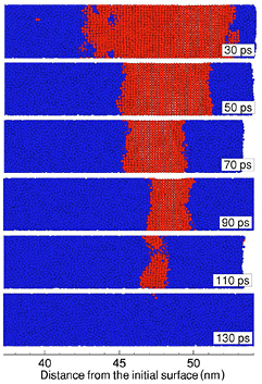
Figure 15. Snapshots of melting of a crystal slightly above melting temperature. Laser and material are the same as in figure 14, however, this figure shows an area at the rear side of the film. Red atoms indicate crystal surroundings while blue regions are molten. Heterogeneous melting is visible as a melting front proceeding through the crystal. The temperature is only slightly above melting temperature, thus the melting front proceeds through the crystal considerably slower than sound velocity. One melting front originates from the rear side of the sample, one has proceeded through fast melting processes from the front side. Reprinted figure with permission from [114], Copyright (2003) by the American Physical Society.
Download figure:
Standard image High-resolution imageThus, both types of thermal melting have been observed in one simulation. Since heterogeneous nucleation of the molten phase appears without any energy barrier at the solid-vapor interface, it occurs on both surfaces. For strong overheating above melting temperature, the gradually proceeding melt front is superimposed by molten nuclei which build homogeneously due to fluctuations. Once a phase transition has started, the melt front further proceeds into regions of lower overheating with temperatures around melting temperature. Recently, both thermal melting processes have also been observed in a simulation of a laser-irradiated semiconductor film [119].
5.2. Nonthermal melting
When a material is excited by high-fluence femtosecond laser pulses, an extreme nonequilibrium state is created, which can live for a couple of picoseconds, see section 1. This state is characterised by the presence of very hot electrons that, after absorbing a large amount of photons from the laser pulse and thermalizing through electron–electron collisions, acquire an extremely high temperature. On the other hand, the lattice still remains cold, since the laser excitation and electron thermalisation occur on a time scale that is generally much shorter than lattice heating through incoherent electron–phonon coupling, which has been described in section 3. Although ions remain at room temperature, they experience strong forces due to the dramatic changes suffered by the potential energy surface (PES), i.e. the effective potential acting on the ions, which depends on the electronic state, after the laser pulse excited a considerable fraction of electron–hole pairs [127, 128]. Thus, ions 'feel' a sudden change of the potential, which leads to the appearance of forces, and start moving. This motion is in most cases cooperative (i.e. the ions do not move independently from each other) and can sometimes even be coherent [129, 130]. Such mechanisms have been reviewed in [131–133].
If the forces arising from the above mentioned changes in the potential energy surface are strong enough, then the material disorders very quickly, even before incoherent electron–phonon heating becomes effective. This ultrafast disordering can be interpreted as melting, which occurs at room temperature. Such phenomenon is called nonthermal melting, and has been studied both experimentally and theoretically since the early eighties [134, 135]. In case sufficient energy is provided by the exciting laser pulse, the material stays in the new phase also after recombination of the electron–hole pairs and/or electron cooling.
The original theory formulated by Stampfli and Bennemann [127, 128] states that the functional form of the potential energy surface (PES) strongly depends on the occupation of the electronic levels. As an example, Stampfli and Bennemann computed the PES along a particular transversal and a particular longitudinal phonon mode at the L-point of the Brillouin zone of silicon. When the electrons are in the ground state, the PES looks like a two dimensional harmonic potential, in which both phonon modes oscillate independently of each other. Now, if 15 of the valence electrons become excited, the PES acquires a form which can no longer be described as a two dimensional harmonic potential. Moreover, in one of the phonon directions it even becomes repulsive (negative curvature), which means that large atomic displacements have to be expected along this direction [128]. Stampfli and Bennemann used for their theory the tight-binding model, which relies on a simple single-electron Hamiltonian. Later, different density functional theory approaches were used to account for the changes in the PES upon electron–hole-pair excitation, which were based on the ideas first developed by Stampfli and Bennemann [136–143]. The basic procedure to obtain the so called 'laser excited ab initio PES' is first to assume that electrons have a particular (usually very high) temperature as a consequence of the excitation and subsequent thermalisation. Thus, electronic occupations are considered to follow a Fermi distribution at the resulting electronic temperature Te. Then, the Kohn–Sham equations are solved self-consistently under this constraint for the electronic occupations. In addition, the electronic entropy at Te is determined. Then, by applying a generalised Born–Oppenheimer approximation, the PES is obtained as
  , where
  are the atomic coordinates,
  the electronic occupations at Te, Ee is the total energy of electrons (which depends on
  ), and Se is the electronic entropy, also depending on the electron occupations. ab initio MD simulations were applied to study laser induced structural changes, in semiconductors like Si [136, 137, 139, 141, 142], Te [144], InSb [140, 145], As [146], semimetals like Bi [138, 147], and metals like Al [139], Au [139], Ag [143, 148] and Cu [143].
In semiconductors, laser pulses create electrons in the conduction band (mostly in antibonding states) and holes in the valence band (mostly in bonding states). As a consequence, the overall bond strength of the material is reduced. This phenomenon is known as laser induced bond softening and has been confirmed by a wide range of experimental studies [149, 150]. While the first experiments were based on optical methods [134, 135], later time resolved x-ray diffraction or x-ray spectroscopy measurements allowed a direct analysis of the lattice order [130, 151–156]. All these results show clear evidence of ultrafast structural changes in different elements, mostly semiconductors and semimetals. Experiments have also revealed rather short melting times of metals after femtosecond laser excitation [124, 125]. However, they could be explained with (homogeneous) thermal melting [123] or other ultrafast destruction mechanisms [157].
The main feature of non thermal melting is the fact that it occurs when atoms are still either at room temperature or at least well below the melting temperature. In the framework of the theory of Stampfli and Bennemann, nonthermal melting should occur when the presence of excited carriers leads to lattice instabilities, represented by imaginary phonon frequencies. All static ab initio calculations agree in the occurrence of lattice instabilities for high enough electronic temperatures. Note that static calculations, based on the calculation of phonon spectra in the laser excited state, cannot predict which kind of lattice instabilities will lead to nonthermal melting. In semiconductors, the first phonons to become unstable are the transversal acoustic ones.
In order to confirm that lattice instabilities lead to nonthermal melting, simulations had to be performed. The first ab initio simulations to describe nonthermal melting of semiconductors were performed by Parrinello and co-workers [136, 137]. Those simulations on Si at constant volume and using a basis set of plane waves yielded a rapid disordering of the lattice structure and convergence of the pair correlation function to that of the liquid state.
It is important to mention that it is experimentally very difficult to characterise nonthermal melting and to distinguish it from ultrafast thermal melting. Therefore, experimental efforts in recent years have been aimed at obtaining information about the trajectories of the atoms immediately after laser excitation. Ultrafast diffraction techniques, based either on x-rays or on electrons, are the most suitable to follow the average atomic trajectories. However, different experiments on semiconductors have led to different and contradictory results. For instance, laser pump x-ray probe diffraction experiments on InSb were interpreted in terms of an inertial model [158]. According to it, the laser excitation leads to a completely flat PES, so that atoms move after excitation with constant thermal velocity corresponding to room temperature. On the other hand, ultrafast electron crystallography experiments performed on Si were compatible with a diffusive motion of the atoms after laser excitation, which is governed by stochastic interatomic collisions. In both experimental studies the time resolution was not small enough to capture possible acceleration of atoms due to lattice instabilities. Recent ab initio simulations performed on larger cells and using the code CHIVES [141, 142], based on Gaussian wave functions, clarified this controversy. According to those simulations, atoms first undergo an acceleration and are then decelerated for a time between half and one picosecond. This subdiffusive motion could be characterised by being fractionally diffusive [142]. Then, after enough interatomic collisions have taken place, the motion becomes purely diffusive, satisfying Einstein's diffusion equation. The onset of diffusion corresponds to the presence of a liquid state [142].
Density functional theory calculations have shown that, in contrast to semiconductors with covalent bonding, ultrafast laser excitation induces bond hardening in metals like gold, copper and silver [139, 143, 148]. However, bond softening or no effects on phonon frequencies have also been obtained for various laser-excited metals [139, 159]. In [160] it was mentioned that the question on bond hardening or softening may depend also on boundary conditions.
5.3. Coulomb explosion
Apart from nonthermal melting discussed in the previous section, another ultrafast phase transition is under discussion, namely Coulomb explosion. This process is known for large molecules or clusters, when highly excited electrons leave the structure. The resulting repulsive forces between the remaining ionised atoms lead directly to destruction of the cluster.
It has been intensively debated whether this process may also be responsible for ablation from large solid samples. Molecular dynamic approaches were used to study the effect of such repulsive Coulomb forces on the crystal lattice [161]. Experimental time-of-flight measurements have found monoenergetic ion beams emitted from irradiated surfaces, which were interpreted as stemming from Coulomb explosion [162]. It is however questionable whether in solids strong electric fields at the surface can be compensated by conduction band electrons from the bulk of the material. The large reservoir of mobile electrons is the main difference from the case of small solid-like clusters.
Bulgakova et al [120] have studied the possibility of electrostatic disintegration of surface layers in detail, by modelling photoelectron emission and electronic transport due to the resulting fields for metals, semiconductors and dielectrics. Typical representations of these material classes have been chosen with gold, silicon and sapphire. It has been assumed that the surface of a bulk material was irradiated with a 100 fs (FWHM) laser pulse. The fluence has been chosen slightly above the respective threshold for ion emission, namely 1.2 J cm−2 for gold, 0.8 J cm−2 for silicon and 4 J cm−2 for sapphire. The resulting electric field in a thin surface layer is plotted over time in figure 16. The calculated field strength for gold and silicon are enlarged by factors of 100 and 50 respectively. However, for sapphire rather large transient electric fields are observed. In [120] a critical field strength necessary to break atomic bonds in sapphire was estimated with help of the latent heat of sublimation for a single atom. The resulting critical electric field is shown in figure 16 as a dashed line. For a short time the calculated electric field at the surface of the dielectric material exceeds this value. Bulgakova et al conclude that Coulomb explosion is possible in dielectrics. Note that a similar amount of emitted electrons have also been obtained in the calculations for metals and semiconductors. However, the resulting space charge was neutralised fast enough, due to the high amount of high-mobility charge carriers in these materials [120]. In [163] experimental results were interpreted with the process of Coulomb explosion also for a semiconductor, namely silicon, which have later been under discussion in [164, 165].

Figure 16. Transient electrical fields in a thin surface layer of a dielectric (Al2O3), a semiconductor (Si) and a metal (Au) respectively. The two latter curves are enlarged. The laser pulse is of 100 fs duration (FWHM) and centered at t = 0. The laser fluence was chosen slightly above the respective ion emission threshold. The electric field in the dielectric temporarily exceeds a certain field estimated as critical for Coulomb explosion. Reprinted figure with permission from [120]. Copyright (2004) by the American Physical Society.
Download figure:
Standard image High-resolution imageThe theoretical results of [120] have been compared with experiments on sapphire [166] concluding that the sharp peak of electrical field at the surface (see figure 16) may be responsible for the observed fast ion emission from the surface marking the onset of ablation. However, the main part of ablation occurs later and is accompanied by a much larger amount of removed particles and the formation of a crater on the target surface [166–168]. The latter ablation regime, also occurring in metals and semiconductors, is the main mechanism determining ultrafast laser ablation. The dynamics of matter expansion will be discussed in the following sections of this review.
6. Hydrodynamic descriptions
Solid matter, which has been excited on a subpicosecond timescale and has undergone ultrafast phase transitions of thermal or nonthermal character (see section 5) is in a highly excited state. The density of such matter is still, in good approximation, solid density—since the expansion is connected with atomic movement and takes much longer time than the ultrafast (thus isochorical) heating and phase transitions with negligible density change. Such state is called warm dense matter; it can also be reached with heating by heavy ions and is the subject of intense research in the fields of planetary science and inertial confinement fusion [169–172].
Here, we first recall a simple expansion model [173, 174], which results in an optically sharp interface of the ablating surface. Such an interface is the key to explaining experimental observations of Newton fringes on the ablating surface [6]. The complete picture of the ablating surface was revealed by further analytical and numerical considerations [175–178]; selected properties of the ablation cupola will be discussed in section 6.2. Finally, extensive numerical approaches, aiming also to simulate the complete ablation process far from ablation threshold, are reviewed in section 6.3.
6.1. Simple expansion model
The initial rapid laser excitation can be viewed as isochoric heating. Equilibration of electron–lattice temperature is generally faster than expansion of the material, which, in turn, is usually fast in comparison with the time scale of heat conduction. Therefore, we consider here adiabatic expansion of matter with a density equal to normal solid density  . We further assume a temperature on the order of the critical temperature of the material and study the expansion of a uniformly heated, semi-infinite layer.
The flow of expanding matter is described by the equations of gas dynamics
where ρ is the density, and p is the pressure of the material which expands in the x direction with the mass velocity u. The set of equations (32) and (33) is completed in the case of adiabatic expansion by the equation of the isentrope  , resulting in a direct dependence of pressure on density,
  . The flow of matter then depends only on the self-similar coordinate x/t [173, 179] and we obtain an implicit equation for the density profile as

Here,  is the local sound velocity, which is the key parameter in the following discussion.
Figure 17 shows the phase diagram of aluminum with four isentropes of different entropy and the isochore of solid state density  . They were taken from the tabulated equation-of-state (EOS) data of aluminum which were constructed by the methods developed in [180, 181]. After the initial rapid isochoric heating (vertical dotted line) by laser excitation, the material is in a state marked by the letter A. Varying excitation strengths lead to different temperatures and pressures within the material, therefore the entropy S at that stage and during the following adiabatic expansion depends on the excitation strength. Expansion occurs along an isentrope, four examples are marked in the figure 17. The solution of equation (34) for these four isentropes is plotted as a density profile depending on the self-similar coordinate x/t in figure 18.

Figure 17. Phase diagram of aluminum with four isentropes and the isochore with solid state density  . The two-phase region (liquid–gas) is shaded. The start values of the temperature of the four isentropes at the solid state density
  have been 10190 K, 7610 K, 5170 K and 3960 K, respectively, from top to bottom. The corresponding start values of the pressure have been 36.5 GPa, 31.3 GPa, 21.2 GPa and 19.8 GPa.
Download figure:
Standard image High-resolution image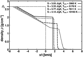
Figure 18. Self-similar solution for adiabatic expansion of aluminum fluid heated isochorically to four different starting temperatures. These have been 10190 K, 7610 K, 5170 K and 3960 K, respectively, from the fastest to the slowest resulting expansion profile. The corresponding expansion isentropes are shown in figure 17.
Download figure:
Standard image High-resolution imageThe square root of the slope of the isentrope is the sound velocity which enters equation (34). Outside the two-phase region the sound velocity of the liquid phase has a comparably large, approximately constant value (note the logarithmic scale of the pressure axis in figure 17). For a constant sound velocity, the self-similar solution (34) yields an exponential expansion profile, this can be compared with the head and the initial part of the rarefaction waves in figure 18. However, the sound velocity decreases sharply when the isentrope enters the two-phase-region [179]. For the isentrope with the smallest entropy, this point at the binodal is marked with the letter B in figure 17. The strong drop of the sound velocity by several orders of magnitude causes a jump in  in equation (34), since the term
  changes rapidly at the moment the density ρ drops below the density at the binodal,
  . Therefore, a plateau of constant density
  appears in the self-similar solution, compare equation (34) and figure 18. More importantly, due to the low value of sound velocity for densities smaller than
  , the self-similar coordinate x/t in equation (34) stays nearly constant with further decreasing ρ. For the
  profile in figure 18, this leads to a steep, step-like density gradient. Note that for higher excitations, a layer of very low density (corresponding to the gas phase) can be observed in front of this step-like density gradient. For the lower entropies considered here, corresponding to lower initial temperatures, the density decreases on a scale of
  10 ms−1. Such a profile is, also after several nanoseconds, steep enough to act as an optically sharp interface.
Here, we have discussed the self-similar profile for the special case of expanding aluminum. In [173, 174] a general qualitative case was discussed, considering a simplified isentrope with two different slopes. The assumed analytical expression for the pressure dependence on such an isentrope was  with
with  for the case of expansion in the liquid phase and
  for the two phase region, reflecting its small sound velocity. Both branches are matched at a certain point (
 ) in the phase diagram, namely on the binodal, compare point B in figure 17. This consideration directly shows that the point (
 ) corresponds to a finite segment in the self-similar representation, building the plateau segment. Its width is given by the difference of the sound velocities
  taken at both respective sides of the binodal point B, while its density equals
  [1, 173, 174].
Note that another mechanism to explain an optically sharp interface was discussed by Bulgakova in [182]. Here, heating and expansion far above the critical point was assumed and a certain curvature of the isentrope led to a rarefaction shock appearing as a sharp front in the density profile. However, as will be discussed in the following section, an optically sharp interface seems to exist in particular close to ablation threshold, thus for lower excitations than assumed in [182].
6.2. Properties of the ablation cupola
Up to now, the expansion of a semi-infinite, uniformly heated material into vacuum has been analyzed. Such condition of a uniform temperature can be fulfilled in a thin film of heated material with thickness  nm [14], compare discussion in section 4. However, when the rarefaction wave hits the unperturbed substrate, i.e. at a time of
  , it is reflected and the self-similar solution loses its validity. Reflection of the rarefaction wave will also occur in bulk material at the non-ablating, shock-compressed internal part of the target.
Figure 19 sketches qualitatively different stages of the evolution of the density profile. Figure 19(a) shows the unperturbed self-similar rarefaction wave with a head travelling with sound velocity  towards the substrate, as shown also in the density profiles in figure 18. After reflection at the substrate, the head of the rarefaction wave travels with the local sound velocity
  in the same direction as the expanding fluid, see figure 19(b). However, when reaching the plateau, the local sound velocity is
  while at the other end of the plateau it is given by the much smaller sound velocity on the two-phase side of the corresponding point on the binodal
  . Therefore, the rarefaction wave will not overtake the plateau and the latter remains nearly unperturbed when moving away from the substrate. It follows directly from mass conservation that the density in the region between the substrate and the plateau must decrease. The resulting density profile at that stage, expected to survive for comparably long time, is sketched in figure 19(c). Numerical gas dynamic calculations [173] as well as molecular dynamic simulations [178, 183] confirm this picture. The latter simulations will be discussed in more detail in section 7.
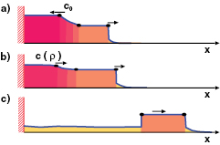
Figure 19. Schematic evolution of the density profile, (a) resulting from self-similar solution, (b) after reflection of rarefaction wave, (c) at the later stage, represented by a moving shell of condensed matter in front of a low-density two-phase region. Figure taken from [184].
Download figure:
Standard image High-resolution imageThe low density region in figure 19(c) consists of two-phase matter, while the high density region is in condensed phase. With increasing fluence the thickness of the two-phase matter increases, while the thickness of the condensed shell decreases. Since the intensity distribution over the focal spot is not uniform but in good approximation follows a Gaussian distribution, the expanding plume takes the shape of a cupola [175–178]. A laser beam of visible light can pass through the shell building this cupola. It can also pass through the low-density region between shell and substrate. This picture therefore represents an explanation for the observation of Newton fringes during ultrafast microscopy of an ablating surface [6].
For high laser fluences, the expansion isentrope enters the two-phase region near the critical point. Here, the drop in sound velocity is less pronounced and the resulting density profile is less steep, compare figures 17 and 18. Therefore, the outer condensed shell of the expansion plume will smear out as time proceeds; first in the center of the Gaussian laser profile, where the largest intensity has excited the target. Figure 20 shows a schematic picture of the fluence profile of the irradiating laser beam (a) and the resulting profile of the expansion plume (b). The point 'ev' in figure 20 marks the rim of the open aperture of the cupola, where the fluence exceeds a critical value Fev for the appearance of a shell of condensed matter. Note however, that a comparably sharp density gradient still exists along the curve '1'. The region in front of the sharp density gradient is filled with vapor 'v'; its thickness increases with increasing fluence [175].

Figure 20. Schematic picture of the expansion plume. (a) Fluence profile of the irradiating laser pulse and (b) resulting profile of crater 'cr', condensed shell 'sh' and two-phase region in-between. The melting threshold 'm' and the disappearance of the shell for high fluence 'ev' are marked as well. Reprinted from [176], Copyright (2007), with permission from Elsevier.
Download figure:
Standard image High-resolution imageIn [184] the limits for the observation of Newton fringes were estimated. The lower limit was identified with an isentrope reaching the binodal at zero or normal pressure, marking roughly the ablation threshold. The upper limit was defined through the sharpness of the density profile of the self-similar solution. It turned out that the ratio of the starting temperatures (at solid density, point A in figure 17) approximately equals the ratio of critical temperature to the boiling temperature at normal conditions,  , which is the relative extension of the two-phase region.
In case of linear absorption two pulses of different fluences heat the target to different temperatures of approximately the same ratio. In order to verify whether our estimations on the thresholds for the observation of the Newton fringes are reasonable, we therefore compare the ratio of the experimentally observed fluence limits of appearance of Newton fringes with the temperature ratio  extracted from EOS data. Table 1 shows these values for various materials. In case the disappearing of Newton fringes was not observed in the experiment, the largest ratio experimentally reached is given.
Table 1. Relative extension of the two-phase region on temperature scale given by the ratio of critical temperature to the boiling temperature at normal pressures,  , together with the experimental fluence ratio for the observation of Newton rings,
  , for different materials.
| Temperature ratio (EOS data) | Fluence ratio (Exp) | |
|---|---|---|
| Graphite | 1.32 | 1.3 |
| Silicon | 1.46 | 1.5 |
| Gold | 3.04 | >4.3 |
| Aluminum | 3.06 | >2.3 |
It can be seen from table 1 that the fluence range for the observation of Newton fringes corresponds to the relative size of the two-phase region. The denoted ratios do not exactly coincide; however, the comparison is satisfactory and supports our explanations for the observation of Newton fringes in near-threshold ablation experiments of different materials. We conclude that the upper limit for the observation of Newton fringes is given by the sharpness of the expansion profile, while the ablation threshold is connected with an expansion isentrope crossing the binodal at approximately zero pressure. The latter assumption has also been verified through molecular dynamic simulations, see section 7.
Note that this picture of ablation close to threshold is universal not only for different kinds of material, metals as well as semiconductors [184, 185], but also independent of the wavelength of excitation, up to the regime of extreme ultraviolet (XUV) [186].
6.3. Simulation of the complete ablation process
There exist a number of hydrodynamic approaches studying distinct features of ultrafast laser ablation, like progression of a pressure wave into the target [178], spinodal decomposition [187], influence of a critical tension on spallation [188], formation of nanoparticles in the ablation plume [189], and many more.
There are also several hydrodynamic simulations aiming to follow the complete ablation process. They incorporate descriptions of the initial excitation and energy dissipation to hydrodynamic approaches in order to include all relevant mechanisms [190–192].
Among them, the work of Colombier et al [190] is particularly interesting, since the influence of certain parameters entering the simulation is systematically studied and the numerical results are directly compared with experimental measurements. In [190] the authors implement the two-temperature model, equations (2) and (3), into an earlier developed hydrocode [193]. They apply a constant coupling parameter α and a thermal conductivity  as given in equation (31). Moreover, they allow changing heat capacities due to changing densities of the solid. This feature is necessary because the authors assume that electron–lattice heating may proceed more slowly than expansion of matter. Thus, heating in this case is not assumed to be necessarily isochoric. In accordance with this assumption, an additional term for the electronic pressure was included in the hydrodynamic equations. The authors compare the calculated ablation depths for copper and aluminum with experimentally measured ablation depths and thresholds. The coincidence is good for fluences well above ablation threshold. However, the simulation overestimates the threshold fluence for copper, while it is underestimated in the case of aluminum. For the case of copper, a parametric variation was performed to analyse the influence of certain parameters entering the model. Namely, the electron–phonon coupling parameter was multiplied by a factor between 0.03 and 30 keeping all other model parameters at the original values. The same was done for the electron thermal conductivity. The results are repeated in figure 21, which shows the threshold fluence for ablation for both cases of parameter variations.
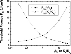
Figure 21. Calculated threshold fluences for different values of the electron–phonon coupling and the electron thermal conductivity, respectively. Results are shown for copper. The original coupling parameter was constant with  , denoted here as
  , and the thermal conductivity
  followed equation (31). Reprinted figure with permission from [190]. Copyright (2005) by the American Physical Society.
Download figure:
Standard image High-resolution imageAn increased thermal conductivity leads to an increased threshold fluence, while an increased electron–phonon coupling decreases the predicted ablation threshold. The physical explanation is straightforward: a better energy confinement and a faster lattice heating leads to higher lattice temperatures at the surface and thus more efficient ablation.
This analysis gives an idea about the accuracy of calculated ablation thresholds. In each simulation, parameters of a distinct uncertainty enter. When the simulation is aimed to provide quantitative predictions of experimentally accessible observables, the influence of such parameters on the finally sought integrated quantity has to be analyzed carefully. Such variations are also a key to understanding the interplay of mutually influencing processes.
The model described in [190] was extended in [191], where the time evolution of electronic pressure and atomic pressure was included in the hydrodynamic model explicitly. It was shown that the electronic contribution to ablation is particularly strong in the first tens of nanometers close to the free surface. The same idea was followed by Chimier et al in [194]. Here, a scenario of instantaneous pressure relaxation was discussed, thus, expansion occurs not only before electron–lattice coupling is completed, but even during ultrafast laser irradiation. The resulting equation-of-state in dependence on electron temperature and lattice temperature was presented. While this EOS reveals a number of generally interesting features, conclusions based on the assumption of instantaneous pressure relaxation on subpicosecond timescales are questionable.
In [192], Povarnitsyn et al simulated ablation of aluminum. They assumed two temperatures in one fluid and connected the TTM with a semiempirical multiphase EOS with separate descriptions of electrons and heavy particles. Expansion and phase transitions far above ablation threshold were studied. For different layers in the expanding material, the thermodynamic trajectories in the phase diagram were followed and material's behavior was analysed. Two different mechanisms of liquid–gas phase transitions were studied, first, bubble growth in metastable liquids and second, fracture of material due to large strain rates. The latter has been shown to be the dominant ablation mechanism. Thus, processes at negative pressure have to be included to gain reasonable comparison with experimental results.
In [195] and [196] the model was further elaborated and applied for various materials. The method allows in particular analysis of the phases of the expanding matter. Figure 22 shows the time-versus-depth plot of expansion. Different colors refer to different phases. White areas are not occupied by any ablating matter. The ablation/movement of gas and liquid clusters to positions outside the inital surface and the formation of a crater at the depth of about 100 nm can be clearly seen. The oscillations on the crater surface between melting and metastable melting (see figure 22) are attributed to elastic (acoustic) oscillations of the thick liquid layer.
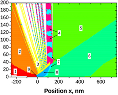
Figure 22. Expansion plane of aluminum after irradiation with a 100 fs laser pulse of 5.0 J cm−2. The laser irradiates from the left-hand side to the surface, which is initially located at x = 0. Different phase states are indicated as: metastable gas (1), metastable liquid–gas mixture (2), metastable liquid (3), metastable melting (4), metastable solid (5), solid (6), melting (7), liquid (8) and stable gas (9). The ablation of the surface as well as the formation of a molten layer on top of the remaining crater can be observed. Reprinted from [195], with permission from Elsevier.
Download figure:
Standard image High-resolution image7. Molecular dynamic simulations
In order to understand the material's behavior after ultrafast heating on the atomic scale, including the kinetics of phase transitions and material removal, molecular dynamic (MD) simulations can be very enlightening.
In this section, we will review a number of calculations which are based on a pre-assumed heating profile. This may not reflect all peculiarities discussed in sections 2–4; the inclusion of these mainly electronically driven effects requires hybrid approaches, which will be discussed in section 8. However, a pre-assumed heating profile may be particularly instructive, when results for different molecular dynamic potentials are compared [175, 177, 197]. Moreover, it allows directly checking the results of MD simulations against those from hydrodynamic descriptions, when in both cases identical initial conditions are assumed. Both kinds of simulation can be insightful in interpreting the results of the respective other and in understanding the physical nature of the particular process under study [176, 178, 183].
For such comparison, informations about density, temperature and pressure should be extracted from the MD simulations. In the following section we briefly sketch the calculation of these averaged quantities and state several advantages of the MD approach. In section 7.2 we will present MD results, which are qualitatively and quantitatively comparable to the hydrodynamic calculations of the ablation cupola discussed in section 6.2. The particular questions of ablation threshold and the thermodynamic pathways of matter in the vicinity of the threshold were successfully addressed with the help of MD simulations; part of these will be reviewed in section 7.3. General discussions of the influence of the applied interatomic potentials are summarised in section 7.4.
7.1. General principles
The classical MD method is based on the solution of a number of Newton's equations, each of them corresponding to the motion of a particular atom. While the underlying equation is thus a rather simple one, the challenge lies in the choice of the interaction potential between the atoms and in the numerical complexity of simulating a huge amount of particles to reflect most realistic macroscopic properties and dynamics of matter.
The simplest example of a potential U used in MD simulations is the Lennard-Jones (LJ) potential,

where  is the distance between the atoms at the respective positions
  and
and  . The energy and space parameters and σ can be determined through comparison with macroscopic properties of matter like the bulk modulus and the equilibrium volume. Note that this determination depends on the choice of these macroscopic parameters as well as on the fitting procedure [198]. The first term in equation (35) essentially corresponds to the repulsive force between atoms while the second term leads to an attractive force at longer distances. Such types of potentials, comprising interactions between pairs of atoms, are called pair potentials. Despite its simplicity, several important results on ablation dynamics have been obtained with large scale MD simulations assuming an LJ interaction potential. Some of these will be reviewed in the following sections.
An important advantage of MD based descriptions as compared for instance to hydrodynamic approaches (see section 6) is the a priori inclusion of nucleation kinetics and phase transitions. In contrast to hydrodynamic descriptions, where an instantaneous [178] or a delayed [192] transition to the two-phase mixture may be assumed, the MD simulations do not have to make any assumptions on nucleation kinetics. On the contrary, important information on the nucleation kinetics are gained from MD calculations. Molecular dynamic methods are therefore particularly suitable in studying fast non-equilibrium phase transitions. For instance when studying the expansion of overheated matter and the resulting density profile in sections 6.1 and 6.2, an instantaneous drop in sound velocity was the basis of the discussion. However, in reality this drop may proceed continuously, since the material proceeds through metastable states. It was in fact an important result of the first large scale molecular dynamic simulations in this context [183] that the general picture of a moving shell in front of a two phase region (see figure 19) also holds when metastable states are inherently included [175, 178, 183].
Quantities like the local density, temperature or pressure are averaged quantities. They can be extracted in MD simulations at each time step of the calculation in order to compare with hydrodynamic or other continuous approaches or to study nucleation kinetics in detail. The local density averaged over N particles, which are typically a small fraction of the total number of simulated particles, is straightforwardly defined through the volume VN, these N particles occupy in the simulation region, thus

The local temperature TN is usually determined with the ideal gas approximation,
where kB is the Boltzmann constant, m the mass of the simulated particles and  the thermal velocity of the particle j, given by the change of its coordinate
  and the center of mass velocity
  of the corresponding computational cell of N atoms. The local pressure is often calculated as a sum of the ideal gas contribution and the virial term as

where  is the force acting on particle j and
  is the distance of particle j from the center of the considered volume [199].
The extraction of such quantities allows direct comparison of molecular dynamic results with hydrodynamic calculations, as performed for example in [178, 183, 197]. Some of these results will be reviewed in the following sections.
7.2. Comparative view on the ablation cupola
Large-scale simulations of the dynamics of 10–100 millions of particles have been performed assuming a Lennard-Jones potential and a semi-infinite target with periodic boundary conditions in two dimensions and free expansion in the third [176–178]. Here, an exponential heating profile has been assumed with its maximum at the free boundary of the simulation region.
Figure 23 shows the evolution of the ablating material, heated from the right-hand side and expanding towards it. From top to bottom different stages of the ablation process are shown, namely a melting front proceeding into the bulk matter, expansion of the surface, formation of a foam (two-phase region) consisting first of bubbles in liquid phase which later coalesce, leading to a droplet–vapor mixture.

Figure 23. Expansion of a semi-infinite Lennard-Jones material, initially heated with an exponential temperature profile. Time proceeds from top to bottom. The expansion can be readily compared with the schematic evolution of the density profile of a heated layer shown in Figure 19. While the top figure shows only a slight surface excursion as compared to the unperturbed material, the lower panels reveal the transition to a two-phase region in the expanding material with a shell of higher density at the expansion front. The bars on the bottom figure mark this high-density shell as well as the position of the remaining crater. Reprinted from [176], Copyright (2007), with permission from Elsevier.
Download figure:
Standard image High-resolution imageThese dynamics reflect the results of hydrodynamic calculations as introduced in the preceding section. Qualitatively, figure 23 can be directly compared with figure 19. The upper picture in figure 23 shows the rarefaction of the material and a sharp density gradient at the expansion front as was found from the self-similar solution of expansion, compare figure 19(a). The gradient conserves as time proceeds and below the surface a phase transition to gaseous phase takes place, forming a foam structure behind a condensed shell moving further outwards. The low-density two-phase region expands and the density is decreasing further, as it was also concluded from the self-similar hydrodynamic calculations, compare figure 19(c). The shell is conserved during expansion. In the bottom picture of figure 23 it is marked with two vertical lines.
Note that in the molecular dynamic simulation the phase transition from solid to liquid (from ordered to disordered state) is also visible. A solid-density region, the boundary of which is also marked in the bottom picture of figure 23, will remain after ablation, forming the bottom of the ablation crater.
Such simulation results of ablation dynamics also compare quantitatively well with results of hydrodynamic approaches [178, 183]. A thorough discussion of the mentioned ablation dynamics comparing hydro- and molecular dynamic simulations qualitatively and quantitatively as well as analyzing them with respect to experimental observations with the help of ultrafast microscopy and interferometry was presented by Inogamov et al in [178].
A complete view of the ablation cupola is represented with expansion pictures for the same instants of time after initial excitation but for different excitation strengths. Figures 24 and 25 show the expansion for decreasing excitation strengths from left to right.

Figure 24. Viewgraphs of the MD results for a Lennard-Jones solid, heated instantaneously with an exponential heating profile and decreasing heating strengths from left to right. The laser irradiates the material from the top; the heating depth is  . The viewgraph on the outermost right represents the unperturbed solid and the initial surface position. The depth in real units is indicated for this simulation on the right axis. A heating strength of
  (here denoted as MDE) corresponds to the ablation threshold. All profiles show the early stage of expansion, when the rarefaction wave has travelled 72% of the heated layer thickness. Figure taken from [178] with permission of Springer.
Download figure:
Standard image High-resolution image
Figure 25. Same as figure 24, for a later stage of expansion, when the rarefaction wave has travelled twice the distance of the heating depth dT. Figure taken from [178] with permission of Springer.
Download figure:
Standard image High-resolution imageFigure 24 represents an early stage of the formation of the liquid shell, which is visible for excitations marked with  and
and  . The temperatures are given in Lennard-Jones units ('moleculardynamic units', MDU), i.e. they are normalised to the energy parameter of the Lennard-Jones potential , whereas the depth scales with σ, see equation (35). Here,
  corresponds to the ablation threshold. The pre-assumed heating profile is exponential with a characteristic length of
  , which corresponds for the applied simulation to a depth of dT = 204 nm. In figure 24 the undisturbed crystal phase can be identified as well as a molten region for lower excitations and a liquid–gas mixture for higher excitations. The threshold for the liquid shell in front of the two-phase mixture as discussed in section 6.2 lies in-between the two highest excitations; for
  no shell but a clear boundary of dense vapor is observed.
Figure 25 shows a later stage of expansion. At that time, droplets in the gas phase have formed, as can be clearly seen for the two highest excitations. On the other hand, in the panel for  , marking approximately the ablation threshold, bubbles have also appeared deep in the material. The physical processes close to ablation threshold are discussed in more detail in the following section. Note that similar viewgraphs of the fluence-dependent expansion profile have also been obtained for an interatomic potential of a metal [200, 201].
7.3. Thermodynamic pathways at ablation threshold
In figure 20 the ablation threshold is marked at a radius of rcr. In contrast to this sketched profile, the material expands continuously in the real experiment. This is also visible in the MD simulation in figures 24 and 25 showing a slight excursion of the material surface also for  , which is slightly below ablation threshold.
The ablation threshold was investigated in detail with the help of MD simulations in [197]. Figure 26 shows the phase-space trajectory of expanding aluminum in the vicinity of ablation threshold. A homogeneously heated slab expands freely in one dimension with laterally periodic boundary conditions. The expansion in both directions leads to overlapping of the rarefaction waves corresponding to the image of a reflected rarefaction wave as discussed in section 6.2 [183]. While in [183] the complete picture of the shell structure could be confirmed for the first time, in [197] the thermodynamic pathway of the central two-phase region was at the focus of the study. To that end, density, pressure and temperature were evaluated for the central third of the simulation volume. The three parts of figure 26 represent different excitation strengths, increasing from top to bottom. In each figure, four isentropes are also plotted, obtained from an aluminum EOS [180]. Note that these isentropes also include metastable states, in contrast to those in figure 17, which are based on the same data.
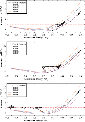
Figure 26. Thermodynamic pathways of expanding aluminum after instantaneous energisation of the energy E0 per atom. Additionally, isentropes are shown, labeled with temperatures corresponding to the initial state at solid density n = n0. The material is heated isochorically to a certain temperature. The starting temperature increases from top to bottom. The expansion was calculated with the help of MD simulation. Each 0.2 ps the pressure and density was monitored and the corresponding point is marked in the respective figure. The black line connects these points to a trajectory of the expanding material in the pressure–density phase diagram. The black arrow on the trajectory close to the initial state indicates the direction of time flow. Reprinted figure with permission from [197], Copyright (2008) by the American Physical Society.
Download figure:
Standard image High-resolution imageThe interpretation of the thermodynamic pathways shown in figure 26 was possible through molecular dynamic snapshots and the relation to the corresponding thermodynamic phases [197]. The upper part of figure 26 shows expansion along an isentrope into a region of negative pressure, i.e. tensile stress, then pressure relaxation connected with contraction, and further acoustic oscillations around zero pressure. The density is reduced as compared to the initial situation, but the material is still in liquid phase. The central figure represents the expansion slightly below ablation threshold. The material expands along an isentrope, reaches metastable states at negative pressure and relaxes to nearly zero pressure. In that state it contains bubbles in a liquid phase. However, the initial energisation was not strong enough for a complete transition into gaseous phase and also, after the observed partial phase transition, the material is still under tensile stress—therefore it contracts again. The final state is thus in liquid phase and no ablation has occurred. The lowest part of figure 26 shows the thermodynamic pathway of aluminum slightly above ablation threshold: the material expands again to negative pressure, the gas phase nucleates while the material is still expanding. Zero pressure is reached, however, in this case it is slightly positive pressure. Therefore, after a short contraction, the material further expands into the gas phase—thus it is ablated.
Note the difference in the timescales of contraction in the two cases below ablation threshold. Each point on the trajectory was determined 0.2 picoseconds after the preceding one. Thus, close to ablation threshold the expansion recovers on a much longer time scale than further below ablation threshold. The timescale of expansion and contraction in the central picture of figure 26 by far exceeds that of acoustic oscillations in the liquid phase. Such long-scale surface excursions in the vicinity of ablation threshold were found experimentally [53, 202] and analyzed with help of hydrodynamic and molecular dynamic simulations [177, 197]. The reason can be attributed to the formation of gaseous bubbles, also below ablation threshold. Recently, a hybrid simulation including fast resolidification has shown that such bubbles can be conserved as a void structure below a re-crystalised silver surface [203].
7.4. Solid potentials
The choice of a suitable potential is crucial in any MD simulation. Usually it is chosen with the aim of describing a real material with a most accurate interaction potential, reproducing known properties like crystal structure, melting temperature or sound velocity. It is likely that any chosen potential works best (meaning most realistically) only in a certain range of temperature, density or pressure. Finding a 'good potential' is a challenging task and beyond the scope of this review.
Instead, we briefly show in this section, which differences have been observed in the previously discussed works, appearing due to the particular choice of the MD potential. For instance, the central panels of figure 25 indicate that gaseous bubbles in expanding Lennard-Jones material appear in the solid phase. The reason lies in a much higher melting temperature of approximately 50% of the critical temperature, than obtained for metal potentials, e.g. aluminum where the melting temperature is only about 10% of the critical temperature [177, 197]. The threshold isentrope leading to ablation of the LJ material may therefore not enter the liquid state [197, 204].
The threshold energies for ablation, as well as those for melting and bubble formation, have been compared for different metals as well as LJ material in [197]. The main difference in the potentials is that the LJ potential is a pair potential whereas the metals were simulated with many body potentials reflecting the delocalised metallic binding. Figure 27 (top) shows the threshold energies for ablation (spallation), as well as those for melting and bubble formation (void) for LJ material and different metals [197]. The energies of initial excitation E0 were normalised to the cohesive energy Ecoh of the material, directly resulting from the applied respective potentials. It can be seen that breaking of the crystal structure is most expensive in terms of energy for the LJ material, whereas the energy range for melting and void formation are smaller than in all considered metals. Differences in melting thresholds were studied on atomistic scale in [177], where the potential barriers for relocation of a single atom in an fcc lattice were analyzed. The energetic costs for such displacement were much lower in aluminum than in LJ material and silicon.
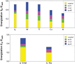
Figure 27. Areas of energisation for reaching different phases upon expansion, normalised to the cohesive energies of the different materials. The thresholds for the respective phases are at energisations corresponding to the bottom of the respective coloured area. The top panel shows the comparison of LJ material to several metals simulated with many body potentials. The bottom panel shows the effect of the size of the simulation region, here thickness of the heated film. Reprinted figure with permission from [197], Copyright (2008) by the American Physical Society.
Download figure:
Standard image High-resolution imageFigure 27 (bottom) shows also a comparison of a small simulation region (30 monolayers, as applied for the simulations presented in section 7.3) with a larger one (300 monolayers, used in the simulations presented in section 7.2). The increase in the thickness of the simulated film has a clear effect on the energy ranges for the observed phases. In particular for the thick film of LJ material the formation of voids appears directly from the solid phase. This behaviour was also observed in [204] and studied in dependence on the crystal's orientation.
It was pointed out in [175] that the transverse dimensions of the simulation region (perpendicular to the direction of expansion) are also important. A better agreement of MD simulations with hydrodynamic calculations has been achieved for larger lateral dimensions.
8. Hybrid approaches
Many modern approaches combine different types of numerical calculations in order to follow the ablation process on a broad range of temporal and spatial scales. Aspects of excitation and energy dissipation on femtosecond to picosecond timescales can be included more or less directly into hydrodynamic calculations. Such hydrocodes aiming to simulate the complete ablation process were reviewed in section 6.3. For the case of molecular dynamic simulations the inclusion of the initial excitation dynamics is more complex, since the electronic system, playing the main role in the initial stage of energy absorption and dissipation, is not included in MD simulations from the first. Even when considering the electrons as classical particles, their inclusion into a MD description is hindered by their small mass and much shorter timescale of their dynamics as compared to the atoms. Therefore, modelling the heating and energy dissipation of the electrons is usually performed in a specially dedicated approach, which can be combined with MD to build a hybrid simulation.
In the present section we focus on the combination of electronic descriptions with molecular dynamic simulations. Such studies allow consideration of effects discussed in sections 2–5 of this review. Note that these simulations are continuously developed and applied for various combinations of laser- and material parameters. Here, we restrict ourselves to presenting the basic principles of such modelling and typical observations of the interplay of electronic behavior and structural modifications enabled with hybrid approaches.
We first discuss a way in which the electronic heat transport can be incorporated in atomistic simulations. This method is most appropriate to describe metals where a large number of electrons provide the energy transport. Results of such simulations are reviewed in section 8.2. To describe excitation and structural dynamics in semiconductors or dielectrics, modified approaches have been performed. Classical electronic descriptions for such materials combined with MD simulation will be presented in section 8.3, while the combination of density functional theory calculations, tracing potential changes upon excitation, with the resulting atomic movement is reviewed in section 8.4.
8.1. Incorporating electron heat transport in molecular dynamics
When heat conduction effects come into play, especially in metals, the electronic heat transport has to be taken into account. A possible way to model such conditions is the combination of the two temperature description with a molecular dynamic simulation. Such hybrid combination was introduced in [205] and further developed in [114, 126, 206]. In these simulations the heating of the electrons by the laser and the further energy dissipation by electron–phonon coupling as well as electron thermal transport is described in the frame of the two temperature model (TTM), while the movement of the lattice atoms is simulated with molecular dynamic (MD) methods. Here we briefly review the principal method as presented in [114].
To combine the two temperature model with a molecular dynamic simulation, the latter equation of the system (2) and (3) was substituted by an equation of motion for the lattice atoms and a coupling term accounting for the lattice heating by the electrons. The resulting equation system reads:


Here, equation (40) has to be solved for each considered atom j with mass mj at position  . The force
  acts on atom j and depends on the chosen interatomic potential. The force
  enters due to electron-lattice heating. The energy received by the lattice is transferred to motion of the lattice ions. This term is balanced with the loss of electron energy
  to ensure energy conservation.
  is directly proportional to the momentum of particle j. In [114] it was shown that the thermal velocity
  has to be considered here, thus
  , where
  is the velocity of the center of mass of the computational cell to which atom j belongs, see section 7.1. The factor ξ which ensures energy conservation, is deduced in [114].
To solve equation system (39) and (40) numerically, the main challenge is to couple a finite difference scheme for the electronic heat conduction with a molecular dynamic (MD) simulation accounting for atomic movement of the surface atoms and a continuum description for the bulk of the material. Figure 28 shows schematically the parts of the model and the energy exchange between them. The MD method is used only in the very surface region of the target, where active processes of laser melting and ablation are taking place. The diffusion equation for the electron temperature is solved in a much wider region affected by the thermal conduction from the absorbing surface layer. In order to avoid reflection of the pressure waves propagating in the MD part from the irradiated surface, a dynamic boundary condition that mimics the interaction of the atoms in the boundary region with the outer 'infinite elastic medium' should be applied [206]. In the outer part the lattice temperature is calculated using equation (3), usually neglecting the ionic heat conduction  .
.
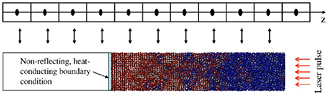
Figure 28. Schematic representation of the hybrid TTM–MD model applied in [114]. The laser irradiates the target from the right hand side. The structural dynamics at the surface region of the target is simulated with MD methods, while the inner part as well as the electron heating and energy dissipation is calculated with the TTM. Both schemes are spatially connected. Reprinted figure with permission from [114], Copyright (2003) by the American Physical Society.
Download figure:
Standard image High-resolution imageThis scheme allows studying the influence of the electron dynamics on structural changes due to laser irradiation. For short laser pulses a prolonged lattice heating can thus be included and in contrast to the studies presented in the preceding section 7 the pre-assumption of a certain energisation of the atoms can be avoided.
8.2. Results for metals
In [114, 126, 206] the hybrid TTM–MD has been developed and kinetics of melting and disintegration of a metal film have been observed on an atomic scale.
In [206] a coherent emission of ablated material was found for laser irradiated copper. This picture is consistent with the observation of Newton fringes [6] and the results of large scale MD simulations applying the simplified LJ potential [178, 183] as reported in section 7. The application of a realistic metal potential in combination with a consideration of the electron dynamics of excitation and relaxation led to a good agreement of calculated ablation thresholds with experiment [206].
In [114] melting and disintegration of free standing nickel and gold films have been studied. Figure 29 shows contour plots of the resulting lattice temperature (a) and pressure (b) for irradiation of a 50 nm nickel film in the vicinity of but above the ablation threshold. A laser pulse of 200 fs duration was assumed to irradiate on the target from the bottom of the plots. On a timescale of a few picoseconds, the lattice temperature and the pressure within the material increase strongly. The onset and completion of melting are marked by black dotted and solid lines respectively. It starts from both free surfaces; however, the melting from the back of the film starts with delay, which results directly from the electronic heat transport assumed in this calculation. Melting kinetics on the atomic scale have been shown and discussed in section 5. Another effect of the implementation of the electron dynamics is the gradual lattice heating. Figure 29(a) shows a temperature increase at the irradiated surface of the film lasting about 20 ps. This timescale is connected with the electron–phonon coupling discussed in section 3. For the calculation of figure 29 a comparably large, constant coupling parameter was assumed. The strong expansion of the film observed on the same timescale leads finally to two voids in the center of the irradiated film. The rupture follows a strong tensile pressure, compare figure 29(b). After disintegration of the film, pressure waves, visible as blue and green zigzag lines, appear in both parts of the disintegrated film.
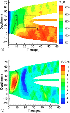
Figure 29. (a) Temperature and (b) pressure contour plots for an excited nickel film, irradiated with an ultrashort laser pulse slightly above ablation threshold. The laser-irradiated surface is at the bottom of the film, depth = 0 nm. The nickel film extends initially to a depth of 50 nm while below and above these depths is vacuum. The solid and dashed lines indicate the region of phase transition to the molten state. The squares show a spatial and temporal area which is discussed in more detail in the original reference [114]. Reprinted figure with permission from [114], Copyright (2003) by the American Physical Society.
Download figure:
Standard image High-resolution imageFigure 30 shows a temperature plot for the similar case of the irradiation of a 50 nm film of gold, irradiated with a 200 fs laser pulse slightly above ablation threshold. We compare it to the case of nickel, figure 29. In gold, the lattice temperature increases for a duration up to 75 ps. The assumed coupling constant was about one order of magnitude lower than that for nickel. Another difference between the two materials appears in the temperature profile. The gold film shows a homogeneous temperature distribution, which is due to a large electronic heat conductivity. As a result, both parts of the disintegrated film are equally heated, while in nickel the disintegration of the film separates a hot front layer from a colder back layer. The effects described above can only be observed in the frame of a TTM–MD description when including a description of electron dynamics as heat transport and electron–phonon interaction in the MD simulation.

Figure 30. (a) Temperature and (b) pressure contour plots for an excited gold film, irradiated with an ultrashort laser pulse slightly above ablation threshold. The geometry and the markers in the figures are the same as explained in figure 29. Reprinted figure with permission from [114], Copyright (2003) by the American Physical Society.
Download figure:
Standard image High-resolution imageResults for a bulk sample of nickel were presented in [207] and are shown in figure 31. The figure shows contour plots of lattice temperature (left plots) and pressure (right plots) for nickel irradiated with a 1 ps laser pulse of increasing fluence from top to bottom, i.e. from (a) to (d). The black line marks in each plot the border between liquid and crystal. For moderate excitations, inducing melting but no ablation, the figure (a) shows heating, heat transport, a pressure wave of positive and negative pressure proceeding into the material and expansion at the free surface. The phase border induces a slight discontinuity for most of these features. For slightly higher fluence, ablation of a single liquid layer is observed, as was also reported in the works reviewed in section 6. A pressure oscillation occurs in the ablated layer, visible in figure 31(b) right-hand side. It appears both in the ablated layer and in the remaining bulk. The surface of reflection of the bulk pressure wave is provided by the liquid–solid interface. Further above the ablation threshold (c) the ablated material consists of several layers or droplets, which are of decreasing size for even higher fluences (d).

Figure 31. Temperature (left) and pressure (right) contour plots of a laser-excited bulk sample of nickel. The initial surface is at depth = 0 nm; vacuum is for positive distances, thus the laser irradiates from the top in each figure. The panels show the extension or ablation of the irradiated surface. The black line in each plot indicates the border between crystalline and molten state. From top to bottom increasing laser fluences, indicated in the respective figure, are applied. The pulse duration was 1 ps. Figure reprinted with permission from [207]. Copyright (2009) American Chemical Society.
Download figure:
Standard image High-resolution image8.3. Approaches for semiconductors
When semiconductors or dielectrics are to be described in the frame of a TTM–MD or similar scheme, the implementation of the electron dynamics becomes more complicated. In these materials, the density of conduction band electrons is not constant (compare section 2), and the transport of heat and also particles has to be considered (compare section 4).
Combinations of the density dependent TTM [34] with molecular dynamic simulations have recently been realised [21, 117, 119]. In [21, 117] the influence of certain parameters and approximations on the resulting dynamics have been discussed. The results of [119] show the interplay of pressure and temperature and their influence on the melting kinetics. Note that ablation has not been studied, since a changing potential energy surface (see section 5.2) has not yet been implemented in this large scale simulation (see sections 5.2 and 8.4).
Another way of implementing carrier dynamics into a MD simulation of semiconductors was chosen in [208]. Here, the authors applied a Monte Carlo approach to account for carrier heating on femtosecond timescales, together with a molecular dynamic calculation of the subsequent atomic displacement on pico- to nanosecond timescales. Picosecond heating followed by expansion up to the nanosecond regime was also investigated. The initial carrier dynamics were taken explicitly into account, including generation and transport of free carriers and phonon emission. The transition from the semiconducting solid silicon to a metallic-like liquid state has also been implemented. It drastically changes the reflectivity of the material (compare section 2). The authors attribute the onset of ablation to a direct conversion of translational mechanical energy into surface energy. The general view of ablating material as well as the pathway in the phase diagram look similar to those in the works reviewed above [178, 183, 197]. Figure 32 shows the near-threshold ablation after femtosecond excitation. Nucleation of a bubble can be observed—due to the small calculation region only one bubble is visible—as well as ablation of a liquid shell.

Figure 32. Near-threshold ablation of a silicon surface after irradiation with a laser pulse of 500 fs duration [208]. Atoms marked with green color belong to the solid phase whereas red atoms have a liquid surrounding. Figure reprinted with permission from [208]. Copyright (2006) by the American Physical Society.
Download figure:
Standard image High-resolution image8.4. Expansion under electronically induced potential changes
Neither of the approaches presented in the previous section implementing electronic excitation in semiconductors to molecular dynamics consider changes of the potential due to electronic excitation. As we have discussed in section 5.2, such changes of the potential energy surface may, however, lead to strong changes of the atomic bonds and should thus be considered in a consistent molecular dynamic simulation, in particular in semiconductors exhibiting strong covalent bonds. The implementation of a transiently changing potential surface into such an approach is, however, challenging. Direct combinations of first principles calculations with MD simulations have been employed by different groups and are mentioned in Chapter 5.
Also, different molecular dynamics simulations including the dynamics of electrons within a tight-binding scheme have been performed, giving insight into the mechanism of laser induced lattice instabilities as a driving force for nonthermal melting. One of those approaches was based on the numerical solution of the time-dependent Schrödinger equation [209–211], whereas in the other approach an equation of motion for the density matrix was solved together with the molecular dynamics [212–216]. In spite of the model character of the tight-binding method, good agreement was obtained with experiments regarding pre-ablation and ablation thresholds in graphite [216] and regarding the dependence of the ablation and melting thresholds in Si as a function of the pulse duration [215]. Figures 33 and 34 show results of such hybrid approach for graphite combining a tight-binding description of electron dynamics with molecular dynamics simulations based on a potential energy surface calculated using the same tight binding Hamiltonian. Incoherent electron–phonon interactions and diffusion were also taken into account, but using a phenomenological approach [216]. In figure 33, a lower excitation has been assumed, which does not show melting of the graphite planes. However, a pre-ablation regime consisting in the successive ejection of intact and ordered planes has been obtained. This result was experimentally confirmed by Zewail and co-workers through ultrafast electron crystallography experiments [217]. The existence of this pre-ablation regime was exploited for producing ultra thin graphitic flakes by femtosecond laser irradiation of graphite [218].
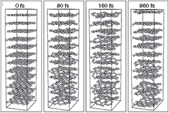
Figure 33. Ablation of single graphite layers after excitation of electrons to an energy of 2.4 eV/atom, which is however still below the damage threshold for graphite planes. The pulse duration was 20 fs. Different instants of time are shown, 0 fs refers to the initial stage. Reprinted figure with permission from [216], Copyright (2001) by the American Physical Society.
Download figure:
Standard image High-resolution image
Figure 34. Complete destruction of the graphite structure after excitation of the electrons to an energy of 4.0 eV/atom, which corresponds to an energisation above the ablation threshold. The pulse duration was 20 fs. Different instants of time are shown, 0 fs refers to the initial stage. Reprinted figure with permission from [216], Copyright (2001) by the American Physical Society.
Download figure:
Standard image High-resolution image
For comparison to the pre-ablation regime, figure 34 shows the complete disorder of the graphite structure on a timescale of about 80 fs, solely due to electronic excitation. A liquid-like state and the ablation of single carbon atoms and chains is observed. Thus transient low density liquid carbon can be produced by laser excitation of graphite [216].
9. Summary and conclusions
In this review, we have presented approaches to modelling ultrafast laser ablation of solids, as well as the underlying processes, on a broad range of timescales. These processes reach from the femtosecond to the nanosecond scale, i.e. from the initial energy absorption to the final material removal.
We have discussed descriptions for laser absorption in metals, semiconductors and dielectrics, focussing on simplified models suitable to serve as initial conditions for further modelling of the induced processes. We have given expressions to describe the energy transfer from electrons to the lattice, mentioning successive electron–phonon collisions as well as a direct influence of electron heating on the interatomic potential. The transport of energy into the depth of the material has been analysed and different descriptions have been compared. Further, ultrafast phase transitions as well as material expansion leading finally to ablation have been described. Common approaches include hydrodynamic models as well as molecular dynamic simulations which yield qualitatively (and sometimes even quantitatively) comparable results. Finally, hybrid simulations aim to combine the mentioned modelling approaches to cover the complete range of timescales from the initial excitation to the final material removal. Here, we have presented the basic principles of a number of such approaches.
In conclusion, ultrafast laser ablation involves a broad variety of processes and effects, each opening an exciting field of research of ultrafast microscopic phenomena in solids. Emerging combined hybrid simulations cannot cover all peculiarities of the distinct phenomena; however, they allow interesting insights on the interplay of these processes.
Acknowledgments
We gratefully acknowledge financial support from the Deutsche Forschungsgemeinschaft through the Emmy Noether Grant RE 1141/11-1, the Heisenberg Grant RE 1141/15-1, and the Projects RE 1141/14-1 and GA 465/16-1, as well as from the Russian Foundation for Basic Sciences through Grants 13-02-01078 and 16-02-00864. We are indebted to many colleagues and coworkers for numerous calculations, analyses and fruitful discussions within the last few years.