
Abstract
X-ray free electron lasers (XFELs) have emerged as powerful sources of short and intense x-ray pulses. We propose a simple and robust procedure which takes advantage of the inherent stochasticity of self-amplified stimulated emission (SASE) pulses to enhance the time-resolution and signal strength of the recorded data. Notably, the proposed method is able to enhance the average signal without knowledge of the signal strength of individual shots. Simple metrics for the probe pulses are introduced, such as an effective pulse duration applicable to SASE pulses characterised in the time domain using e.g. an X-band transverse cavity. The approach is evaluated using simulated and real pulse data in the context of ultrafast electron dynamics in a molecule. Utilising H2 as a model system, we demonstrate the efficacy of the method theoretically, successfully enhancing the predicted nonresonant ultrafast x-ray scattering signal associated with electron dynamics. The method presented is broadly applicable and offers a general strategy for enhancing time-dependent observables at XFELs.

Original content from this work may be used under the terms of the Creative Commons Attribution 4.0 license. Any further distribution of this work must maintain attribution to the author(s) and the title of the work, journal citation and DOI.
1. Introduction
In recent years, ultrafast chemistry and physics have seen many exciting advances due to the emergence of short and bright x-ray pulses generated by x-ray free-electron lasers (XFELs). One notable example is non-resonant ultrafast x-ray scattering (UXS) of isolated molecules in the gas phase [1–4], which has evolved rapidly since the initial proof-of-principle experiments [5–9]. A summary list of achievements includes the observation of alignment [7, 10–13], tracking of nuclear dynamics during photochemical reactions [6, 14–18], excited state molecular structure determination [19, 20], detection of ionisation and charge states [14, 17], and measurement of the rearrangement of electrons in electronically excited states [20, 21]. These experimental advances have been accompanied by significant theoretical groundwork [22–35] and the development of computational tools crucial for the analysis and interpretation of the experiments [13, 36–43].
Most XFELs use a phenomenon known as self-amplified spontaneous emission (SASE) [44–46]. This process is initiated when a bunch of electrons enters an undulator at velocities close to the speed of light. The alternating magnetic fields in the undulator cause the electrons to oscillate transversely, leading to emission of photons along the direction of travel. Initially, the photons are emitted incoherently. However, interaction between the electrons and the electric field of the photons cause the electrons to emit increasingly in phase, resulting in short, intense, and at least partially coherent laser pulses.
The initial electron bunches, before acceleration to nearly the speed of light, are generated by photoejection. This process introduces stochasticity into the x-ray pulses. As a consequence, the temporal intensity profiles of the x-ray pulses fluctuate significantly. Some pulses will have a longer pulse duration and therefore reduce the overall temporal resolution of the experiment. Likewise, other pulses will have shorter effective durations, with the capacity to, at least in principle, improve the time-resolution in the experiments. Crucially, by using an X-band transverse cavity (XTCAV), it is possible to measure temporal intensity profiles of individual pulses [47–49]. In this paper, we demonstrate how shot-by-shot characterisation of the x-ray pulses using XTCAV data makes it possible to filter out shots with long pulse durations to enhance the overall temporal resolution of the experiment and improve the signal.
This completely general procedure, applicable to any type of time-resolved experiment which utilises SASE XFELs, is illustrated using the imaging of coherent electron dynamics by UXS as an example. Such yet to be realised experiments are likely to benefit greatly from the presented approach since the required time-resolution for resolving electronic motion is high, typically on the order of a few femtoseconds down to attoseconds. Encouragingly, attosecond lasing was recently demonstrated in the soft x-ray regime at an XFEL [48, 50–55] and attosecond pulses in the hard x-ray regime are likely to follow, setting the stage for the eventual measurement of electron dynamics by UXS. Notably, already in currently available SASE pulses, individual pulses can have quite short effective durations. This, combined with the improved repetition rate at next generation XFEL facilities, indicates that the filtering technique proposed in this article could play an important role in future experiments, realising measurements of electron dynamics by scattering, specifically, and improving the time-resolution in a wide range of experiments more broadly.
Electron dynamics manifests in UXS alongside elastic and inelastic scattering contributions to the signal [56–65]. The respective new component in the total, energy-integrated scattering signal arises from the interference of scattering amplitudes from two or more coherently populated electronic states and is therefore sometimes referred to as coherent mixed scattering (CMS) [66, 67]. Measuring CMS poses an experimental challenge, not only because it places high demands on temporal resolution, but also because the CMS signal is weak compared to the elastic and inelastic components. A high signal-to-noise ratio is therefore required in order to measure CMS. Using the methodology proposed in this manuscript, which selects which shots to keep when averaging detector images based on the characteristics of the individual x-ray probe pulses, could therefore dramatically increase the chances of successfully detecting CMS experimentally by enhancing temporal resolution and maximising the CMS signal.
Our conceptual and computational study utilises both synthetically generated and experimentally measured SASE pulses to calculate CMS signals from a vibronic wavepacket in . Although this system is not an ideal candidate for an actual experiment, the hydrogen molecule constitutes a valuable model system for which CMS has been studied in great detail using idealised Gaussian x-ray pulses [66, 67]. These previous results provide a useful benchmark for the signals calculated in the present work. The analysis presented in this paper constitutes a proof-of-concept for a data processing and analysis methodology which could enhance the CMS signal in future experiments. Furthermore, while our focus here is on CMS, the methodology presented is completely general and could straightforwardly be utilised to enhance time-dependent observables across various experiments that employ SASE pulses.

2. Theory
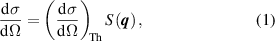
The quantity measured in non-resonant UXS is the differential scattering cross section per solid angle Ω,
where is the differential Thomson scattering cross section of a free electron and is the molecular scattering at momentum transfer vector , where k0 and are the wave vectors of the incoming and scattered photons, respectively. Describing the light–matter interaction with quantum electrodynamics and first-order time-dependent perturbation theory and assuming that rovibrational transitions are not resolved, the molecular scattering for a perfectly aligned molecule is, [66, 67]


where is the photon number intensity of the x-ray pulse at time . Wfij is a weight obtained by the convolution of the pulse's power spectral density with the window function for the detector [68].


The double sum over the indices and in equation (2) runs over all populated electronic eigenstates that arise from the excitation of the molecule prior to scattering and the Born–Huang-type expansion of its wavefunction,


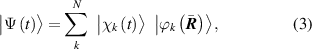
where is the nuclear vibrational wavepacket on electronic state , which depends on the set of internal nuclear coordinates , where is the number of internal coordinates considered.


Finally, is the one-electron scattering matrix element. Its square modulus gives the probability of a transition from the initial electronic state to final state due to a photon scattering with momentum transfer vector q, assuming that the Waller–Hartree approximation is valid [69]. It relates to the real-space one-electron (transition) density through a Fourier transform from real into reciprocal space,


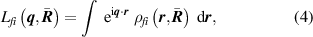
where is the imaginary unit and r the electronic coordinate.

It is instructive to consider the contributions to equation (2). The equation can be split into three distinct contributions depending on the indices , , and . The first is the electronically elastic contribution with . The second is the electronically inelastic contribution with . The third, and most important for this work, is the coherent mixed contribution with and any . The coherent mixed component is accordingly given as,


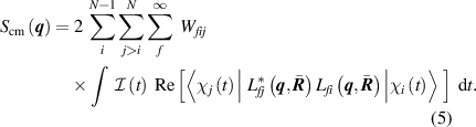
Equation (5) shows that CMS arises from the interference of scattering amplitudes from different populated electronic states, and . Furthermore, the intensity of the coherent mixed term maps onto the square root of the degree of electronic coherence . This is in contrast to the elastic and inelastic components, which are weighted by the populations of the individual electronic states. Because the phase of an electronic state is contained within the nuclear wavepacket in the Born–Huang-type expansion in equation (3), will contain an oscillating term with a frequency , where is the difference in energy between the electronic states with indices and and is the reduced Planck's constant. This relationship demonstrates the close connection between CMS and coherent electron dynamics.


Considering the convolution by the photon number intensity in equation (5) is important for the possibility of detecting CMS given the rapid evolution of electronic wavepackets, generally speaking. If the dynamics is faster than the pulse duration, which is given by the temporal width of , the CMS signal will be averaged out. At the same time, the presence of in equation (5) means that shot-by-shot variations in the SASE pulses will directly impact the magnitude of the CMS signal.


3. Computational methods
3.1. Modelling SASE pulses
To realistically account for temporal intensity profiles of SASE pulses in the simulations, it is necessary to model the pulses' stochastic nature. For this we employ the partial-coherence method shown to emulate the temporal structure of SASE pulses seen in experiments [70, 71]. This allows us to generate temporal intensity profiles, in equations (2) and (5), that display substantial shot-by-shot variation, yet still have a well-defined Gaussian-shaped average.

The partial-coherence method defines the temporal intensity profile as , where the partially coherent electric field amplitude is [72],


Here, is a normalisation factor that ensures that the total energy of the pulse takes a particular value and does not fluctuate across different shots. The electric field is incoherent,


with an initial electric field in frequency-space, , which serves as a starting point and can be expressed as,

The exponential term in equation (8) is the coherence function containing the coherence time and defines, via its Fourier transform, the frequency spectrum of the pulse. The cosine accounts for the rapid oscillation of the electric field with carrier frequency .


Moreover, in equation (7) is a phase factor which takes a different value for each point on the frequency grid in the range . This has the effect of giving each frequency component in the pulse a random phase and, after the Fourier transform, results in an incoherent electric field that has a random shape in the time domain.


Finally, in equation (6) is a Gaussian filter function,


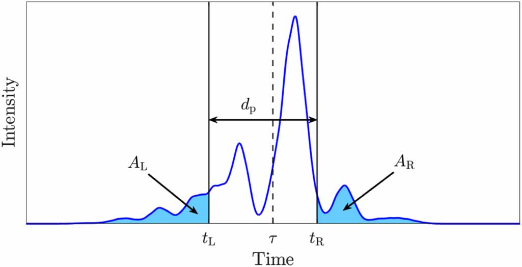
which defines the shape that the average pulse will take. Here, is the centre of the Gaussian and is its full-width half-maximum (FWHM). The purpose of the filter function is to confine to a certain region in the time domain, taking the completely incoherent electric field and making it partially coherent. An example of a pulse generated by the partial-coherence method is shown in figure 1.


Figure 1. An illustration of the parameters used to characterise the temporal intensity profile of SASE pulses. The times and define the pulse duration and τ is the pump–probe delay time (see text for definitions). The areas and are the integrals of from to and from to , respectively. They take the value for a normalised pulse.


Download figure:
Standard image High-resolution image3.2. Pulse characterisation
To sort and select the SASE pulses, it is necessary to define parameters that reliably characterise the shape of each individual intensity profile. Here, we present definitions for an effective pulse duration and a pump–probe delay time τ, which are analogous to the parameters that define an idealised Gaussian pulse.

For a transform-limited pulse with a Gaussian-shaped intensity profile, the duration is usually defined as its FWHM. We define the respective times at which the intensity of the Gaussian pulse equals half its maximum as and . For a SASE pulse, however, these times cannot be rigorously defined via the value of because can, in principle, take any value at any point in time. Instead, and are defined via the integral of from to , , and the corresponding integral from to , . For a normalised Gaussian-shaped pulse, these integrals take the values . In analogy, for a SASE pulse, we determine and numerically such that and take the same value as for a Gaussian pulse. The pulse duration is then simply calculated as the difference . Notably, this definition reproduces the standard FWHM duration for a Gaussian pulse. The approach is illustrated in figure 1.


The delay time τ can be thought of as the centre of the x-ray probe pulse. For a Gaussian, it is simply the time where the intensity is at its maximum. For SASE pulses, this is usually not the case, and τ is better described by the expectation value,
3.3. Simulating ultrafast UXS in H2
To investigate the effect that the stochasticity of SASE pulses has on the CMS signal, scattering signals are calculated according to equation (5). The simulations use previously published electronic potential energy curves, one-electron scattering matrix elements, and nuclear wavepackets [66, 67]. The nuclear wavepackets have been propagated by numerical integration of the time-dependent Schrödinger equation using the WAVEPACKET code [73] in MATLAB [74], with accurate potential energy surfaces, transition dipole moments, and derivative non-adiabatic coupling matrix elements from Wolniewicz et al [75–78]. The one-electron scattering matrix elements, defined in equation (4), are calculated using our own code [39, 79, 80] from electronic wavefunctions obtained using the state-averaged complete active space self-consistent field method with a large active space and basis, SA-CASSCF(2,30)/d-aug-cc-pVQZ, in MOLPRO [81] for the first nine electronic singlet states of molecular hydrogen.
In the published simulation, an extreme ultraviolet pump pulse centred at excites the molecule in its electronic and vibrational ground state, . This pulse has a Gaussian shape with a FWHM duration of 25 fs, a mean photon energy of 14.3 eV, and an electric field amplitude of 53.8 MV . It leads to a partial excitation from the electronic and vibrational ground state, , with 10% of the population transferred to the first electronically excited state, . The electronic coherence between these two states peaks at and the resulting reference CMS signal is calculated for a Gaussian-shaped x-ray pulse. The geometry of the calculations are such that the bond vector of the molecule is aligned with the laboratory axis, the incident x-ray pulse propagates along the axis, and the scattering patterns are calculated in the plane. Finally, the weights are modelled by a box function centered at the mean photon frequency ω0 with a width Δω chosen to justify the truncation of the sum over final states f in equation (5) at the nine electronic states included.


While the previous work of Simmermacher et al approximated the SASE pulse by a simple bandwidth-limited Gaussian function, in this article more realistic temporal intensity profiles are used. Synthetic SASE pulses are generated applying the partial-coherence method discussed in section 3.1, using the following parameters: , , , and . The intensity of the pulse is assumed to be sufficiently low that non-linear processes can be ignored (see SI for further details). The random phases, , were generated using the built-in random number generator in Matlab, initialised by a seed based on the current time. We note that pulse durations on the order of attoseconds are significantly shorter than what is currently available at XFEL facilities. However, these values are needed in order to resolve the fast electron dynamics in H2. Experimentally recorded SASE pulse intensity profiles, scaled down to an average duration of 100 as, are also used for the calculations in section 4.2. Strictly speaking, shorter SASE pulses would most likely undergo qualitative changes, but for the current purpose of matching the overall duration of the pulses to the time-scale of the theoretical model, such linear scaling is sufficient. The method is directly applicable to any SASE pulse as long as its structure is measured and characterised. We also note that the XTCAV measures pulse energy and converting this to intensity requires that the focus diameter is estimated.


4. Results
4.1. CMS with SASE pulses
To compare CMS signals from different SASE pulses with the signal obtained with the idealized Gaussian pulse in previous work, we introduce a scaled signal,
where is the CMS signal calculated according to equation (5) with a realistic SASE pulse and is the reference CMS signal simulated with a Gaussian pulse with the same parameters as the Gaussian filter function in equation (9). The function max(...) in the denominator gives the maximum value across all values of , providing a global normalisation of the CMS signal.


Figures 2(A) and (C) show two examples of scaled CMS signals. The overall shapes of the scattering patterns are identical and do not deviate from the pattern obtained with the Gaussian pulse. They only differ in their magnitudes. We can therefore represent each shot by the maximum value of the respective signal,

The CMS pattern shown in figure 2(A) has a maximum intensity of , which is notably weaker than the corresponding value for the reference Gaussian pulse, . This 25% reduction in intensity is a direct consequence of the intensity profile of the corresponding synthetic SASE pulse shown in figure 2(B). The pulse has an effective pulse duration of , which is significantly longer than the duration of the idealised Gaussian pulse of . Hence, the temporal resolution is decreased, consequently leading to a weaker signal. The signal in figure 2(C), in contrast, is considerably stronger with , which is nearly a 20% improvement over the reference. In this latter case, the underlying SASE pulse in figure 2(D) has a shorter effective pulse duration of only .


Figure 2. ((A) and (C)) Contour plots of scaled CMS signals in the plane. ((B) and (D)) Temporal intensity profiles of SASE-pulses (blue curves) used to calculate the corresponding CMS signal to the left, plotted with the Gaussian filter function (red curves). On the horizontal axes, the time is shifted by the delay time of the filter function . The intensities are normalised to one.


Download figure:
Standard image High-resolution imageFigure 3(A) shows the values of for 25 000 shots simulated with different synthetic SASE pulses and sorted according to the pulse properties that were introduced in section 3.2 The shots are distributed in a circle centred at and , i.e. the FWHM and the centre of the Gaussian filter function. This circular shape is a consequence of the statistical distribution used in the partial-coherence method. As illustrated in figure 3, depends strongly on the effective pulse duration , with shorter pulses unsurprisingly giving stronger CMS signals. This is further exemplified by two pulses with and , which are shown in figures 3(B) and (C). These two pulses lead to quite weak and quite strong signals with and , respectively, as shown by the corresponding markers in figure 3(A).


Figure 3. (A) Distribution of the values of for 25 000 SASE pulses as a function of their delay times τ and pulse durations , with each point representing the value of for a single shot. The values of are shifted (re-centered) by the delay time of the filter function . The colourbar represents the maximum intensity of the CMS signal in terms of . ((B)–(E)) Temporal intensity profiles for four representative SASE pulses (blue curves) shown together with the Gaussian filter function (red curves) for reference. As in (A), the time is shifted by . The values of and the boundaries of are indicated for each pulse and the profiles are normalised to unit area. The marker in the top right corner of each panel is used to identify the corresponding point in panel (A).


Download figure:
Standard image High-resolution imageThe magnitude of the CMS signal also depends on the delay time , reflected by the curved appearance of the blue, yellow and red distributions in figure 3(A). The SASE pulse in figure 3(D) illustrates the effect. Even though this pulse has a shorter than average duration of , it still results in a weak signal with because the pulse is shifted to the shorter delay time of . Here, the signal is weaker simply due to the phase of the electronic wavepacket. Essentially, the measurement is performed at a time when the CMS signal is weak. This is due to the fact that the centre of the Gaussian filter function is set to because the CMS signal reaches its maximum at that time. Hence, any deviation of from that value of inevitably results in a weaker signal.


Interestingly, the SASE pulse in figure 3(E) has an average effective pulse duration of and is centred at , but nevertheless results in a weakly enhanced signal with . This can be explained by the presence of a sharp peak in around and suggests that the manner in which we characterise the pulses cannot fully account for the distribution of the intensity within the boundaries of . We note that the characterisation may be straightforwardly improved by the introduction of additional parameters such as, for instance, a second pulse duration defined by a different width, e.g. the full-width 3/4-maximum (see SI for details). In the latter case, the two integrals and used to determine via and (see section 3.2) take the value .


4.2. Enhancement of the CMS Signal
Next, we consider how one may apply the above pulse characterisation to an actual XFEL-based experiment to enhance the magnitude of ultrafast signals. For that, the synthetic SASE pulses are replaced with real experimental pulse envelopes taken from XTCAV data measured at the CXI instrument of the Linear Coherent Light Source at SLAC in 2021 (proposal number LV04). The intensity profile of the average pulse from this data is shown in figure 4. It displays a largely Gaussian-like shape with two extra shoulders at negative times that together span about 10 fs and has an effective pulse duration of .


Figure 4. Plot of the intensity profile of the average pulse from the XTCAV data as a function of time , with the respective pulse centre and the boundaries of the pulse duration .


Download figure:
Standard image High-resolution imageTo be usable within the currently employed model of attosecond electron dynamics of , the experimentally characterised pulses are compressed in time by two orders of magnitude to an average duration of . Moreover, the centre of each individual pulse is determined according to equation (10) and shifted to a random value within the range to emulate a temporal jitter [82] of 60 as with an average time delay = 62.92 fs. As expected, this random shift leads to a uniform distribution of pulses in , which can be seen in figure 5(A). The overall dependence of the signal strength on the effective pulse duration in figure 5(A) is identical to the one shown in figure 3(A). The distribution is, however, slightly shifted to lower values of . This can be explained by the asymmetry of the average intensity profile seen in figure 4. Because the average intensity has a strong peak at positive values of , individual pulses give stronger CMS signals on average when they are slightly shifted to negative values of .


Figure 5. (A) Distribution of values for 50 000 time-compressed experimental SASE pulses, characterised in terms of their delay times and pulse durations . Each point represents a single shot and the values of are shifted by the average delay time . The colourbar represents the maximum magnitude of the corresponding CMS signal in terms of . (B) The mean improvement in the CMS intensity, plotted as a percent increase in the signal against the percent of shots used, with the limit of 0% shots used corresponding to all shots having been discarded. The blue curve is obtained when shots are eliminated on the basis of , while the red curve shows the results when is used for filtering (an ideal but experimentally not realizable filter).


Download figure:
Standard image High-resolution imageNow, an upper limit for the pulse duration is introduced and only CMS signals simulated with pulses shorter than this limit are averaged. Figure 5(B) demonstrates how the magnitude of the average signal increases as the limit for decreases and more pulses are discarded. Using only 50% of all shots, for example, the strength of the average signal is increased by 10.8% relative to the average with all shots included. By adding a second pulse duration to the characterisation as described earlier, the signal enhancement may be further improved to 11.2% (see SI for details). As a result of this selection, the magnitude of the average CMS signal can be enhanced without prior knowledge about the magnitude of the CMS signal itself. This is particularly useful considering that the signal cannot be determined for individual shots due to its inherent weakness and insufficient signal-to-noise ratio. The CMS signal can only be discerned once averaged over a sufficient amount of shots. This also points to another important aspect of this analysis: the enhancement of the signal comes at the cost of discarding data. Since there is a requirement for a particularly good signal-to-noise ratio in order to detect a significant and discernible signal, a balance must be struck to ensure enough data is kept for the signal to emerge from the background noise.


Even though the intensity of the CMS signal cannot be measured experimentally for individual shots, in the current analysis the theoretical CMS intensities can be used to create a benchmark for the pulse selection based on . Figure 5(B) also shows how the strength of the average signal increases if shots are selected according to their maximum signal . This selection shows a similar trend as the one based on the effective pulse duration before, but there is a significant difference in magnitude, illustrating that there is still room for improvement. For example, selecting 50% of all shots based on yields an increase of 13.5% relative to the average with all shots included, compared to the 10.8% increase previously achieved when using for the selection. The largest contributor to this difference is the dependence on because the temporal jitter of 60 as covers a significant part of the electronic wavepacket's period of . This illustrates the well-known fact that the temporal jitter and the pulse duration jointly impose a limit on the temporal resolution of a pump-probe experiment. The impact of the temporal jitter becomes more significant the fewer shots are used and the lower the average pulse duration is. Hence, a smaller temporal jitter will increase the effectiveness of the shot selection by since the jitter will be less of a limiting factor.


5. Conclusions
We demonstrate that the inherent stochasticity of the SASE process can be exploited to increase temporal resolution by measuring the pulse profiles and systematically selecting short-duration pulses. To achieve this, a simple, robust, and easy-to-implement method for determining effective pulse durations is introduced. The approach is evaluated both on synthetic pulses, generated using the partial-coherence method, and on scaled, experimentally measured SASE-pulses. The method is shown to enhance the difficult-to-measure CMS signal in model calculations of the molecule H2, offering a route to increasing the chance of detecting CMS in experiments that rely on SASE x-ray pulses.

We note that H2, although a useful model system, is not a strong candidate for an actual experiment due to the rapid sub-femtosecond electron dynamics, which would be exceptionally challenging to resolve, and due to the small scattering cross section. Moreover, the simulated CMS signal vanishes if an energy-integrating detector is used [67]. When targets for prospective experiments are selected, these constitute important considerations. One potential candidate for measurements are non-adiabatic transitions at conical intersections, since transient electron dynamics at a conical intersection can be comparatively slow due to the near-degeneracy between the electronic states [59, 60, 62]. However, in that scenario one must carefully consider the symmetries at the intersection [83]. Nevertheless, future simulations of CMS in complex systems will provide an interesting opportunity to further test the data analysis methodology presented in this paper.
In summary, we present an efficient approach for increasing the temporal resolution and enhancing weak transient signals at SASE-based XFELs. No changes in how the experiment is done are required, as long as pulses are characterised on a shot-by-shot basis. Compared to more sophisticated ghost-imaging approaches proposed for increasing temporal resolution [84], the advantage of this approach lies in its simplicity and robustness. The utility of the approach is demonstrated computationally by enhancing a weak CMS signal of a model system, indicating the potential utility of the approach in the context of challenging measurements of coherent electron dynamics in photoexcited systems. Importantly, we note that the approach presented is applicable in a much broader context, providing a way to enhance signals in any SASE-based experiment where the temporal resolution is critical.
Acknowledgments
EML acknowledges a PhD Studentship of the UK XFEL Physical Sciences Hub funded by the Science and Technology Facilities Council (STFC). MS and AK acknowledge funding from the Engineering and Physical Sciences Research Council (EPSRC) EP/V006819/2. AK further acknowledges funding EP/V049240/2, EP/X026698/1, and EP/X026973/1 from the EPSRC, RPG-2020-208 from the Leverhulme Trust, and support from the U.S. Department of Energy, Office of Science, Basic Energy Sciences, under award number DE-SC0020276. PMW was supported by the U.S. Department of Energy, Office of Science, Basic Energy Sciences, award number DE-SC0017995. Data from LCLS beamtime LV04, 'Ultrafast Ghost Imaging of Molecular Dynamics in Ionic Systems', is gratefully acknowledged.
Data availability statement
The data cannot be made publicly available upon publication because no suitable repository exists for hosting data in this field of study. The data that support the findings of this study are available upon reasonable request from the authors.