
Abstract
We employ the Markov approximation and the well-known Fresnel-integral to derive in 'one-line' the familiar expression for the Landau–Zener transition probability. Moreover, we provide numerical as well as analytical justifications for our approach, and identify three characteristic motions of the probability amplitude in the complex plane.
Export citation and abstract BibTeX RIS

Original content from this work may be used under the terms of the Creative Commons Attribution 4.0 license. Any further distribution of this work must maintain attribution to the author(s) and the title of the work, journal citation and DOI.
1. Introduction
Exact solutions of problems in quantum mechanics [1] are rare: the harmonic oscillator, the hydrogen atom, and the Landau–Zener transition [2–6] immediately come to mind. However, even these elementary models require complex mathematics. Especially the derivation of the Landau–Zener 3 transition probability is rather involved, independent of the approach pursued. An integration in the complex plane [2, 8–10], the asymptotic expansion of the parabolic cylinder functions [4, 11–13], or the introduction of a superadiabatic basis [14–17] represent only a few of the many sophisticated techniques [18–24] that eventually lead to the well-known elementary result.
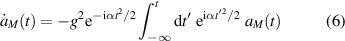
Despite its simplicity [25, 26] there does not seem to exist a 'one-line' derivation of it 4 . This fact is astonishing especially in view of the numerous applications [27–31], and further developments of this model [32–36]. In this note we present such an argument based on the Markov approximation of the resulting Schrödinger equation for the transition probability amplitude.
Our article is organized as follows: in order to set the stage for our insight we define in section 2 the Landau–Zener problem and then derive the relevant equations of motion for the two probability amplitudes which are of first order in time and coupled. When we formally solve for one and substitute the result into the equation of motion for the other we arrive at a first order integro-differential equation.
This equation forms the starting point of our one-line derivation presented in section 3. Here the crucial step is to ignore the memory of the transition probability amplitude which leads us immediately to the familiar asymptotic expression.
We then dedicate section 4 to a justification of the Markov approximation by casting the corresponding integral into a form which verifies the validity of our approach. This formulation also demonstrates that the Landau–Zener transition represents a jump between two circular motions in the complex plane of different radii. We bring out this fact in section 5 by a simplification of the integral governing the dynamics in the Markov approximation.
Finally, in section 6, we transform the Markov integral into yet another form which highlights the difference between negative and positive times. Indeed, we identify the origin of the Stueckelberg oscillations which only appear for positive times due to the interference of two contributions to the Landau–Zener probability amplitude. We conclude in section 7 by briefly summarizing our results and providing an outlook. In particular, we present another one-line derivation based on the corresponding differential equation of second order for the complex-valued probability amplitude.
2. Formulation of the problem
The Hamiltonian
for the two states  and
and  whose energies change with the rate α linearly in time t and are coupled by the Rabi frequency g, leads via the Schrödinger equation
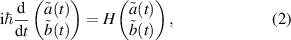
and the introduction of the transformed probability amplitudes  and
and  to the set


of two coupled differential equations of first order. Here the dot denotes differentiation with respect to time.
When we solve formally equation (4) for b, subjected to the initial condition  , and substitute this expression into equation (3) for a, we arrive at the integro-differential equation
Obviously the dependence of the probability amplitude a(t) on the integration variable tʹ is the complication.
3. One-line derivation
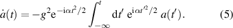
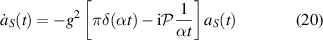
It is at this point that our one-line derivation starts. We perform the Markov approximation [37, 38]  which allows us to integrate immediately the resulting differential equation
subjected to the initial condition  , providing us with the asymptotic transition probability amplitude

Here we have introduced the two-dimensional integral
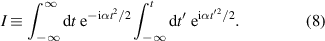
In the decomposition
of I the second contribution vanishes since the integrand is anti-symmetric, and the first term is the product of two Fresnel integrals
leading us to the expression
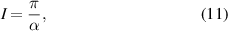
and with equation (7) we arrive indeed at the celebrated Landau–Zener formula
It is surprising that the Markov approximation yields immediately the exact result which is difficult to obtain by other methods. This feature is confirmed by figure 1 where we compare and contrast the time dependence of the probability amplitude a with and without the Markov approximation. On the left we depict this trajectory in the complex plane and note that both curves start out in the same way, then deviate slightly but eventually return to the same end point, demonstrating that the Markov approximation provides us indeed with the exact result
5
. On the right we depict this comparison for the amplitude  and the phase
  as a function of time in more detail confirming again this amazing property.
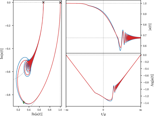
Figure 1. Comparison of the time dependence of the probability amplitude of a Landau–Zener transition with (red line) and without (blue line) the Markov approximation represented in the complex plane (left) and in amplitude  and phase
  (right). Here we have chosen the parameters g = 0.25 and α = 0.5 and have scaled time in units of the coupling frequency g. The open circle (green) marks t = 0. A slight difference between the numerical and the approximate curve occurs in the transition from the circle of radius unity (grey dotted curve), determined by the initial condition
  and indicated by the right cross on the real axis, and the final circle (grey dotted curve) governed by the asymptotic value
  depicted by the left cross on the real axis for positive t. However, the two curves agree perfectly for
  as shown on the right. In the right column we use a logarithmic time on the horizontal axis in order to bring out the different behaviours during the time evolution. Hence, the Markov approximation yields the exact transition probability.
Download figure:
Standard image High-resolution image
4. Validity of the Markov approximation
In order to gain deeper insight into the validity of the Markov approximation we now combine the two quadratic phase factors in equation (5) and introduce the integration variable  leading us to the alternative yet exact representation
of the time evolution of the probability amplitude a.
In the limits of  and τ ≠ 0 the first phase factor in the integral of equation (13) is rapidly oscillating and only contributes in the neighbourhood of τ = 0, that is at the lower limit of the integral. For this reason we can evaluate
  at τ = 0 and factor a(t) out of the integral providing us with a justification for the Markov approximation. Thus, equation (13) reduces to
It is interesting to see how the Landau–Zener formula, equation (12), follows from the integral in equation (14) compared to the one in equation (6). Needless to say both must lead to identical results because they are different representations of the same integral. Nevertheless, we can gain additional insight from equation (14).
Indeed, by integration subjected to the initial condition  we find the asymptotic probability amplitude

where we have introduced the integral
When we interchange the order of integrations we obtain the Fourier representation of a Dirac-delta function δ in the variable ατ together with a factor of 2π which allows to perform the integration over τ, and taking into account that due to the restriction τ > 0, we obtain a factor  .
.
As a result, we arrive at
in complete agreement with equation (11) and thus at equation (12). We emphasize that the integration over τ with the delta function at τ = 0 replaces the quadratic phase factor in the integral over τ in equation (16) by unity.
5. Landau–Zener transition as a jump between two circular paths
The emergence of the delta function is crucial in obtaining the transition from the initial probability amplitude unity to the final value given by the Landau–Zener formula. This fact stands out most clearly when we recall that the main contribution to the integral in equation (14) arises from τ = 0.
Thus we can replace the phase factor quadratic in τ by unity arriving at
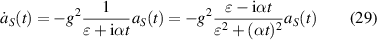
Here we have introduced the subscript S to express the fact that we have made an additional approximation which is valid in the asymptotic regimes  .
.
The identity
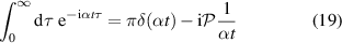
containing the delta function and the Cauchy principal value denoted by  transforms immediately equation (18) into
with the solution
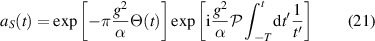
where Θ denotes the Heaviside step function and  .
.
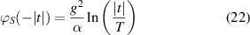
The asymptotic motions corresponding to equation (21) for  when represented in the complex plane are two circles with the radius unity for
  , and the radius given by the Landau–Zener probability amplitude, equation (12), for
  as shown by the grey lines in figure 1. The phase
  of
of  is always negative except at the starting and the end point where it vanishes.
Indeed, we find from equation (19) immediately
and with the integral relation
the result
where the first integral in equation (23) vanishes.
When we differentiate the asymptotic phases ϕS given by equations (22) and (24) we find the angular velocities
and
which for t < 0 is negative but for t > 0 is positive. Moreover, for  the angular velocity approaches zero.
6. Stueckelberg oscillations
From figure 1 we note that for positive t an additional phenomenon emerges: circular motions of ever decreasing radii along a circular path in the clockwise direction terminating on the real axis at  .
.
This feature stands out most clearly when we complete the square in equation (13) leading us to the exact formula
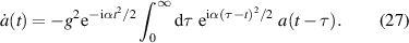
Indeed, for t > 0 the quadratic phase factor in the integral, is slowly varying in the neighbourhood of  . In this case we can replace
  by a(0) and factor it out of the integral.
The resulting contribution is an addition to the one arising from the lower boundary of the integral, and governed by equation (14). The two contributions interfere [15] giving rise to the Stueckelberg oscillations [5]. We emphasize that this qualitative argument requires a more sophisticated approach to obtain good agreement between an approximate but analytic expression for the Stueckelberg oscillations and the numerically exact result.
7. Conclusions and outlook
In this article we have presented a one-line derivation of the familiar Landau–Zener formula based on the Markov approximation and have discussed the validity of our approach. Moreover, we have identified in the exact as well as the Markov dynamics of the probability amplitude three characteristic behaviours in the complex plane: (i) a motion along a circle in the clock-wise direction starting from the real axis at  . (ii) A transition from the original unit circle to the final circle with a radius determined by the asymptotic probability amplitude
  , and (iii) circular motions of decreasing amplitude as
  . We have briefly analysed these motions and, in particular, have derived approximate but analytic expressions for a in these domains of the dynamics.
Several extensions of our approach suggest themselves: (i) solve approximately the differential equation of second order

following by differentiation of equation (5) in the three characteristic time domains. (ii) Analyse the equations of motion for amplitude and phase corresponding to equation (28), and (iii) simplify the nested integrals which emerge when we iterate equation (5), and add up the corresponding sum. We already have performed these tasks but postpone our results to a future publication.
As a small appetizer of coming attractions we point out that the Landau–Zener transition in the form of a delta function with a Cauchy principal value apparent in equation (21) emerges from equation (28) when we neglect the second derivative and add a small real part  to the coefficient in front of
  , leading us to the relation
which in the limit of  reduces to equation (20). Hence, we have found another one-line derivation of the Landau–Zener result.
Acknowledgments
Bruce Shore was a highly gifted physicist with a very deep understanding of quantum mechanics. He discovered many phenomena which will always be intimately connected with his name. Due to his outstanding scientific achievements he enjoyed the greatest respect among colleagues worldwide. However, Bruce was also a multi-talented artist who delighted and touched the people as an outstanding musician with his superb banjo playing, and also as a great draftsman with his ever-popular Christmas cards and his cartoons from his student days at MIT shown at the beginning of every chapter in his last book [41]. Above all he was a wonderful human being who enjoyed life, travelling and collaborating with everybody in the world. Since Bruce loved simple explanations we have chosen this one-line derivation of the Landau–Zener formula for our tribute to his memory.
We thank P B Boegel, M A Efremov, A Friedrich, B M Garraway, P Hänggi, M Holthaus, V Malinovsky, F Nori, B Pacolli, J Seiler, S N Shevchenko, K-A Suominen and S Varro for many fruitful discussions, E M Chudnovsky for reminding us about his prize for an elementary derivation of the Landau–Zener formula, and P Kofman for making [31] available to us before publication.
W P S is most grateful to Texas A&M University for a Faculty Fellowship at the Hagler Institute for Advanced Study at Texas A&M University and to Texas A&M AgriLife for the support of this work. The research of the IQST is financially supported by the Ministry of Science, Research and Arts Baden-Württemberg.
Data availability statement
The data that support the findings of this study are available upon reasonable request from the authors.
Footnotes
- 3
Since Ernst Carl Gerlach Stueckelberg and Ettore Majorana have derived similar results at the same time as Landau and Zener several authors suggest [7] to call these transitions 'Landau–Zener–Stueckelberg–Majorana transitions'. Although we feel that this change is well justified, throughout our article we subscribe to the traditional expression.
- 4
During the workshop honouring Daniel Greenberger and Myriam Sarachik on 22 March 2013 Eugene Chudnovsky mentioned in his presentation that for years he has offered a prize of 1000 $ to his doctorial students for a short derivation but none succeeded and he did not have to pay.
- 5