Keldysh ionization theory of atoms: mathematical details

Optical field ionization of atomic systems has two limiting cases. Tunnel ionization, or the quasi-static limit, occurs when the field remains frozen during the ionization process [1, 2]; when the field varies substantially, multi-photon ionization dominates, see figure 1.

Zoom In Zoom Out Reset image size

Keldysh developed a seminal theory of optical field ionization that comprises both limiting cases, the tunneling, and the multi-photon limit [3]. Dominance of the two ionization mechanisms is determined by the Keldysh parameter

$$\begin{equation}\gamma =\frac{\omega \sqrt{2{I}_{0}}}{F}.\end{equation} \tag{ 1 }$$

Here, ω is the laser circular frequency, F is the laser electric field strength, and I₀ is the ionization potential. Tunnel ionization dominates for γ ≪ 1, whereas multi-photon ionization is dominant for γ ≫ 1. For an intuitive overview of these regimes see [4], and for an overview of other regimes, see [5].

Keldysh's work [3] along with similar work by Faisal [6] and Reiss [7] are sometimes referred together as KFR theory [8], here we focus on Keldysh's formulation. Keldysh's work, is based on the strong field approximation; the wave function is represented as a superposition of an s-bound state (l, m = 0) and the non-relativistic, laser dressed free electron wavefunction in the dipole approximation and the length gauge; by contrast, Faisal and Reiss theories are calculated in the velocity gauge. Keldysh-type theories assume a strong linearly polarized cw laser field of relatively low frequency compared to the atomic ionization potential. As a result of these assumptions, the effect of the far-range Coulomb potential on the continuum electron and on ionization is neglected. Therefore, in the low frequency limit ω → 0, the Keldysh ionization rate does not go over into the (static) tunnel ionization rate [1, 2], as it should. Whereas Keldysh gave a simple Coulomb correction factor, a more sophisticated correction was developed subsequently in the Perelomov–Popov–Terent'ev (PPT) approach [9], where also ionization rates for l, m ≠ 0 [9, 10] were derived (for a comprehensive review of this 'imaginary-time' method, see [11]). Further, for high Rydberg states with large n the original approach becomes inaccurate and corrections have to be added [12]. For detailed reviews of optical field ionization of atomic systems, see [5, 13–16]. Recently, some technical issues with regard to employing saddle point integration versus residue theory in Keldysh's ionization theory were discussed [12, 17, 18] and the original approach was confirmed. For reviews, see [14, 16].

The Keldysh approach to ionization has remained relevant to date. Although it is being widely used, many of its mathematical methods and intricacies are not fully explained. This is unfortunate, as the methodology is of relevance for current research in strong field physics including, for example, attosecond science and [19–21]. Other subsequently explored phenomena include above-threshold ionization [22, 23] and more complicated ionization pathways like non-sequential double ionization [24]. For summaries of other applications involving strong field physics, including those involving novel molecular and solid state systems see [5].

This work does not contain new results. It started as a comprehensive exam question, driven by the authors' desire to understand the mathematical details of Keldysh's derivation of strong field ionization in atoms [3]. Our efforts are complementary to previous work exploring details of Keldysh ionization theory in atoms [12, 16, 18]. Our tutorial is presented in the hope that it will be of use for a wider audience in the fields of strong laser field physics and attosecond science and will entail an even deeper appreciation of Keldysh's brilliant work.

We have adopted most of Keldysh's notation. Atomic units are used to keep the notation simpler. Following the more modern literature [25], P is used as canonical momentum instead of p in Keldysh. For the same reason we have reserved S for the classical action and use T instead of S in (16) and (18) of [3]. Finally, we use t instead of T as a time variable.

The derivation of the Keldysh ionization rate for the ground state (n = 1, l = 0) of a hydrogen-like atom starts from the Schrödinger equation. The laser electric field is accounted for in dipole approximation and in length gauge,

$$\begin{equation}i{\partial }_{t}{\Psi}(\mathbf{x},t)=\left({H}_{0}-\mathbf{x}\mathbf{F}(t)\right){\Psi}(\mathbf{x},t),\end{equation} \tag{ 2 }$$

where Ψ is the wavefunction, ${H}_{0}=-(1/2){\nabla }^{2}-\sqrt{2{I}_{0}}/\vert \mathbf{x}\vert$ is the field free Hamiltonian, F(t) = F cos(ωt) is the laser electric field, and |F| = F.

(2) is solved by utilizing the strong field approximation; the ansatz

$$\begin{equation}{\Psi}(\mathbf{x},t)=a(t){e}^{i{I}_{0}t}\left\vert 0\right\rangle +\int {d}^{3}pb(\mathbf{p},t)\left\vert \mathbf{p}\right\rangle \end{equation} \tag{ 3 }$$

consists of a ground state part fulfilling the time independent Schrödinger equation, ${H}_{0}\left\vert 0\right\rangle =-{I}_{0}\left\vert 0\right\rangle$ with ground state energy −I₀ and wavefunction $\left\vert 0\right\rangle =1/\sqrt{\pi {a}_{0}^{3}}\,\mathrm{exp}(-\vert \mathbf{x}\vert /{a}_{0})$. Here, ${a}_{0}=1/\sqrt{2{I}_{0}}$ is the atomic radius, with a₀ = 1 for a hydrogen ground state (I₀ = 1/2). The ground state probability amplitude a(t) ≈ 1 is assumed to remain frozen which is a good approximation as long as ionization is weak. The second part of (3) is an expansion of the continuum wavefunction in terms of plane waves |p⟩ = 1/(2π)^3/2exp(i px) with mechanical momentum p; b(p, t) represents the continuum electron probability amplitude.

The strong field ansatz (3) introduces three approximations: first, excited bound states are neglected. Second, loss of ground state population due to ionization is disregarded. Third, the effect of the Coulomb potential on the continuum part of the electron wavefunction is not accounted for.

Inserting ansatz (3) into (2), utilizing the Schrödinger equation for the ground state, neglecting the Coulomb interaction for the free electron part, and applying ⟨p'| to the resulting equation yields

$$\begin{equation}i{\partial }_{t}b(\mathbf{p},t)=\!\left(\!\frac{{\mathbf{p}}^{2}}{2}\!-\!i\mathbf{F}(t){\nabla }_{\mathbf{p}}\!\right)\!b(\mathbf{p},t)\!-\!{\mathbf{V}}_{0}(\mathbf{p})\cos (\omega t){e}^{i{I}_{0}t}.\end{equation} \tag{ 4 }$$

Here, we have relabelled p' → p for notational convenience, and inserted the definition of F(t). Further, ${\mathbf{V}}_{0}(\mathbf{p})=\mathbf{F}\left\langle \mathbf{p}\right\vert \mathbf{x}\left\vert 0\right\rangle$ is the potential energy associated with the laser driven transition from ground state to continuum. Following [26] (see also the supplementary material for a derivation) one obtains

$$\begin{equation}{V}_{0}(\mathbf{p})=-i\frac{{2}^{7/2}{(2{I}_{0})}^{5/4}}{\pi }\frac{\mathbf{F}\mathbf{p}}{{({p}^{2}+2{I}_{0})}^{3}}.\end{equation} \tag{ 5 }$$

The dipole term differs by a factor (2π)^3/2 from Keldysh due to the normalized definition of the plane wave states.

Integration of (4) is performed by transforming into a moving momentum frame P = p + A(t), where P is the canonical momentum and A(t) = −(F/ω)sin(ωt) is the vector potential defined by −∂_t A(t) = F(t). The equation of motion in the transformed frame is

$$\begin{equation}i{\partial }_{t}b(\mathbf{P},t)=\frac{1}{2}{\mathbf{P}}_{t}^{2}b(\mathbf{P},t)-{V}_{0}({\mathbf{P}}_{t})\cos (\omega t){e}^{i{I}_{0}t},\end{equation} \tag{ 6 }$$

where P_t = P − A(t). Integration of (6) results in

$$\begin{equation}b(\mathbf{P},t)=i{\int }_{0}^{t}\!d{t}^{\prime }{V}_{0}({\mathbf{P}}_{{t}^{\prime }})\cos (\omega {t}^{\prime }){e}^{-\frac{i}{2}{\int }_{{t}^{\prime }}^{t}{\mathbf{P}}_{\tau }^{2}\,d\tau +i{I}_{0}{t}^{\prime }}.\end{equation} \tag{ 7 }$$

The ionization rate is determined by w₀ = ∫d³ P∂_t |b(P, t)|²; inserting (7) we find

$$\begin{align}\hfill {w}_{0}& =\underset{t\to \infty }{\mathrm{lim}}\int \!{d}^{3}\!P{V}_{0}^{\ast }({\mathbf{P}}_{t})\cos \,\omega t{\int }_{0}^{t}\!d{t}^{\prime }{V}_{0}({\mathbf{P}}_{{t}^{\prime }})\cos \,\omega {t}^{\prime }\hfill \\ \hfill & \quad \times \mathrm{exp}\left(-i{\int }_{{t}^{\prime }}^{t}{I}_{0}+\frac{1}{2}{\mathbf{P}}_{\tau }^{2}\,d\tau \right)+\mathrm{c}.\mathrm{c}.,\hfill \end{align} \tag{ 8 }$$

where the rules of scattering theory are applied; the perturbation is switched on at time zero and the scattered state is analyzed at t → ∞, where a steady state ionization rate has been reached [27]. We proceed by inserting the definition of F(t) and A(t) in (8) and obtain

$$\begin{align}\hfill {w}_{0}& =2\,\underset{t\to \infty }{\mathrm{lim}}\,\mathrm{R}\mathrm{e}\!\int \!{d}^{3}\!P\!\!{\int }_{0}^{t}\!\!d{t}^{\prime }\,\cos (\omega t)\cos (\omega {t}^{\prime }){V}_{0}^{\ast }\hfill \\ \hfill & \quad \times \left(\mathbf{P}+\frac{\mathbf{F}}{\omega }\,\mathrm{sin}(\omega t)\right){V}_{0}\!\left(\mathbf{P}+\frac{\mathbf{F}}{\omega }\,\mathrm{sin}(\omega {t}^{\prime })\right)\mathrm{exp}\hfill \\ \hfill & \quad \times \left(-i{\int }_{{t}^{\prime }}^{t}{I}_{0}+\frac{1}{2}{\left(\mathbf{P}+\frac{\mathbf{F}}{\omega }\,\mathrm{sin}(\omega \tau )\right)}^{2}d\tau \right),\hfill \end{align} \tag{ 9 }$$

in agreement with (8) in Keldysh [3], but with an extra factor of 2 that is missing in Keldysh's manuscript. The prefactor 1/(2π)³ in Keldysh is contained here in the two dipole moments. The symbol Re represents the real part.

Next, a Fourier expansion of the integrand is performed. To that end we reexpress the ionization rate as

$$\begin{align}\hfill \begin{aligned}\hfill & {w}_{0}=\!2\,\underset{t\to \infty }{\mathrm{lim}}\,\mathrm{R}\mathrm{e}\!\!\int \!\!{d}^{3}\!P\,\cos (\omega t){L}^{\ast }(\mathbf{P},t)\!{\int }_{0}^{t}\!\!\cos (\omega {t}^{\prime })L(\mathbf{P},{t}^{\prime })d{t}^{\prime }\hfill \\ \hfill & L(\mathbf{P},t)={V}_{0}\left({\mathbf{P}}_{t}\right)\mathrm{exp}\left(i{\int }_{0}^{t}\!\!{I}_{0}+\frac{1}{2}{\mathbf{P}}_{\tau }^{2}\,d\tau \right).\hfill \end{aligned}\end{align} \tag{ 10 }$$

The Fourier series expansion of L(P, t) and the corresponding coefficients L_n are given by

$$\begin{equation}L(\mathbf{P},t)=\!\!\sum\limits _{n=-\infty }^{\infty }\!\!\!{L}_{n}(\mathbf{P})\mathrm{exp}\left(i{{\Omega}}_{n}t\right)\end{equation} \tag{ 11a }$$

$$\begin{equation}{L}_{n}(\mathbf{P})\!=\!\frac{\omega }{2\pi }\!{\int }_{0}^{{T}_{0}}\!\!\!L(\mathbf{P},t)\mathrm{exp}\left(-i{{\Omega}}_{n}t\right)dt\end{equation} \tag{ 11b }$$

with ${{\Omega}}_{n}=\left({\tilde{I}}_{0}+{\mathbf{P}}^{2}/2-n\omega \right)$, ${\tilde{I}}_{0}={I}_{0}+{\mathbf{F}}^{2}/(4{\omega }^{2})$, and T₀ = 2π/ω the optical cycle. The first two terms in Ω_n are the non-sinusoidal contributions of the exponent in (9) and (10) which have been separated out.

The time integral in (10) is performed by using (11a) and by replacing cos with exponentials resulting in frequencies Ω_n±1. The summation index is redefined so that Ω_n±1 → Ω_n . The ionization rate contains a double sum coming from the expansion of L(P, t) and L*(P, t). Only terms with the same index fulfill energy conservation and result in ionization. All other terms are of virtual nature and do not contribute to net (cycle-averaged) ionization. Their neglect eliminates one of the sums. The resulting integral is divergent in the limit t → ∞ and must be modified to be well defined,

$$\begin{align}\hfill {w}_{0}& =\frac{1}{2}\,\mathrm{R}\mathrm{e}{\int }_{-\infty }^{\infty }\!\!{d}^{3}\!P\sum\limits _{n=-\infty }^{\infty }{\left\vert {L}_{n+1}(\mathbf{P})+{L}_{n-1}(\mathbf{P})\right\vert }^{2}\underset{\varepsilon \to {0}^{+}}{\mathrm{lim}}\hfill \\ \hfill & \quad \times \underset{t\to \infty }{\mathrm{lim}}{\int }_{0}^{t}{e}^{-(i{{\Omega}}_{n}+\varepsilon )(t-{t}^{\prime })}\,d{t}^{\prime }.\hfill \end{align} \tag{ 12 }$$

The time integral for t → ∞ becomes

$$\begin{equation}\underset{\varepsilon \to {0}^{+}}{\mathrm{lim}}{\int }_{0}^{\infty }{e}^{-(i{{\Omega}}_{n}+\varepsilon )\tau }\,d\tau =\underset{\varepsilon \to {0}^{+}}{\mathrm{lim}}\,\frac{-i}{{{\Omega}}_{n}-i\varepsilon }=\pi \delta ({{\Omega}}_{n})-i\mathrm{P}\frac{1}{{{\Omega}}_{n}}\end{equation} \tag{ 13 }$$

with P denoting Cauchy's principal value (PV) [28, 29] which gives an imaginary contribution in (12) that drops out. Further, in the last equality of (13) the Sokhotski–Plemelj theorem is used [29, 30].

The δ-function in (13) in combination with the definition of L_n , (11b), yields the relation

$$\begin{equation}{L}_{n\pm 1}(\mathbf{P})\!=\!\frac{\omega }{2\pi }\!{\int }_{0}^{{T}_{0}}\!\!\!L(\mathbf{P},t)\mathrm{exp}\left(\pm i\omega t\right)dt.\end{equation} \tag{ 14 }$$

Use of relations (13) and (14) in (12) results in

$$\begin{align}\hfill \begin{aligned}\hfill {w}_{0}& =2\pi {\int }_{-\infty }^{\infty }{d}^{3}\!P{\left\vert L(\mathbf{P})\right\vert }^{2}\sum\limits _{n=-\infty }^{\infty }\delta ({{\Omega}}_{n}),\hfill \\ \hfill L(\mathbf{P})& =\frac{1}{2\pi }{\int }_{0}^{2\pi }\!\!\!L(\mathbf{P},x)\cos (x)dx,\hfill \end{aligned}\end{align} \tag{ 15 }$$

in agreement with (14) of [3]; the variable transformation x = ωτ was used and L(P, x) is defined in (10). As the Fourier transform is periodic, integration over any 2π interval can be used.

The second part of (15) is rewritten with the help of variable transformations sin(x) = u, so that cos(x)dx = du, and $dx=du/\cos (x)=du/\sqrt{(1-{u}^{2})}$. We obtain

$$\begin{equation}L(\mathbf{P})=\frac{1}{2\pi }\oint {V}_{0}\left(\mathbf{P}+\frac{\mathbf{F}}{\omega }u\right)\mathrm{exp}\left(\frac{i}{\omega }S(u)\right)du\end{equation} \tag{ 16a }$$

$$\begin{equation}S(u)=\!{\int }_{0}^{u}\!\left[{I}_{0}+\frac{1}{2}{\left(\mathbf{P}+\frac{\mathbf{F}}{\omega }v\right)}^{2}\right]\frac{dv}{\sqrt{1-{v}^{2}}}\end{equation} \tag{ 16b }$$

which agrees with (15) of Keldysh [3]. The above variable transformation is not bijective, i.e. for a given value of u, x is not single valued. This problem can be dealt with in two ways. First, the integration path in (15) can be split in intervals for which the exponent is single valued. Alternatively, the integral can be analytically continued into the complex domain, where with the help of a branch cut the exponent is made single valued, see the dogbone contour in figure 2. This is discussed in more detail in appendix A. We follow Keldysh and continue the contour into the complex plane, and deform it in a way that it passes through the saddle points, see figure 2, which yield the dominant contribution to the ionization rate. This is discussed next.

Zoom In Zoom Out Reset image size

The exponent of the integral in (16) contains a function of u. The first derivative dS/du can be seen as a local frequency which varies with u. The points at which dS/du = 0 are called saddle points; the phase factor exp(iS/ω) remains approximately constant in the vicinity of these points. Away from the saddle points, |dS/du| grows and exp(iS/ω) becomes rapidly oscillating. The integral over a rapidly oscillating phase tends to zero asymptotically according to the Riemann–Lebesgue lemma [31]. As a result, the dominant contribution to the integral comes from the vicinity of the saddle point. A quantitative evaluation of the accuracy of the saddle point method does not exist. However, Keldysh theory has been tested extensively over the past decades and has shown to be quite reliable over a large range of laser and atomic parameters.

In the following we go through the technical details. The first step of saddle point integration consists of expanding the phase to second order about the saddle points u_s± [28]; the yields S(u) ≈ S(u_s±) + S'(u_s±)δu + (1/2)S''(u_s±)δu² with prime and double prime indicating first and second derivatives and δu = (u − u_s±). The main contribution to the integral comes from the saddle points at which S'(u_s±) = 0,

$$\begin{equation}{S}^{\prime }(u)=\left[{I}_{0}+\frac{1}{2}{\left({P}_{z}+\frac{F}{\omega }u\right)}^{2}\!\!+\frac{1}{2}{P}_{\perp }^{2}\right]\frac{1}{\sqrt{1-{u}^{2}}},\end{equation} \tag{ 17a }$$

$$\begin{equation}{I}_{0}+\frac{1}{2}{\left({P}_{z}+\frac{F}{\omega }{u}_{s\pm }\right)}^{2}\!\!+\frac{1}{2}{P}_{\perp }^{2}=0.\end{equation} \tag{ 17b }$$

Here, we have assumed $\mathbf{F}=F\hat{\mathbf{z}}$, and have introduced the longitudinal and transverse momenta P_z and P_⊥ = (P_x , P_y ); further, ${P}_{\perp }^{2}={P}_{x}^{2}+{P}_{y}^{2}$ and ${P}^{2}={P}_{z}^{2}+{P}_{\perp }^{2}$. From (17b) we obtain $({P}_{z}+\frac{F}{\omega }{u}_{s\pm })=\pm i\sqrt{2{I}_{0}+{P}_{\perp }^{2}}$; the ± sign represents saddle points for the positive and negative laser half cycle. The second derivative is found to be

$$\begin{equation}{S}^{{\prime\prime}}(u)=\frac{F}{\omega }\frac{{P}_{z}+\frac{F}{\omega }u}{\sqrt{1-{u}^{2}}}+{S}^{\prime }(u)\frac{u}{1-{u}^{2}},\end{equation} \tag{ 18a }$$

$$\begin{equation}{S}^{{\prime\prime}}({u}_{s\pm })=\pm i\frac{F}{\omega }\frac{\sqrt{2{I}_{0}}}{\sqrt{1-{u}_{s\pm }^{2}}}.\end{equation} \tag{ 18b }$$

After saddle point integration, S''(u_s±) will end up as pre-exponential. We only carry along exponential transverse momentum dependence, which is why ${P}_{\perp }^{2}$ has been neglected in the numerator of (18b). As a result, the phase S(u) is approximated as

$$\begin{equation}S(u)\approx S({u}_{s\pm })\pm i\frac{F}{2\omega }\frac{\sqrt{2{I}_{0}}}{\sqrt{1-{u}_{s\pm }^{2}}}\delta {u}^{2}.\end{equation} \tag{ 19 }$$

The rules of saddle point integration dictate that the integration contour is deformed to pass through u_s± and that δu is chosen along the path of steepest descent. We make the ansatz δu = u − u_s± = s  e^iφ and insert it in (19). Further, $1/\sqrt{1-{u}_{s\pm }^{2}}$ is split into amplitude and phase term ±exp(iζ) with phase ζ defined in the positive imaginary half plane. The two saddle points are mirror points in the positive and negative imaginary half plane for which the phase differs by π, see appendix A. This yields

$$\begin{equation}\frac{i}{\omega }S=\frac{i}{\omega }S({u}_{s\pm })\mp \eta {s}^{2}\,{e}^{2i\varphi }\left(\pm \,{e}^{i\zeta }\right),\end{equation} \tag{ 20a }$$

$$\begin{equation}\eta =\frac{F\sqrt{2{I}_{0}}}{2{\omega }^{2}}\left\vert \frac{1}{\sqrt{1-{u}_{s\pm }^{2}}}\right\vert .\end{equation} \tag{ 20b }$$

The signs in (20a) cancel so that each saddle point gives the same contribution in the second term. The path of steepest descent is determined by φ = −ζ/2. With this choice the last term in (20a) results in a Gaussian decay (steepest descent) in (16). Further, as the saddle point is dominantly imaginary, see (28) further down, ζ ≈ 0 and the path of steepest descent is close to parallel to the real axis. Finally, as the Gaussian expansion in the integrand decays quickly, the integral is extended to ±∞, where the vertical parts of the closed contour integral have no contribution, see figure 2.

Inserting the above in (16a) one arrives at

$$\begin{equation}L(\mathbf{P})\!=\!\frac{1}{2\pi }\sum\limits _{{u}_{s\pm }}{\int }_{\mp \infty }^{\pm \infty }\!\!\!{V}_{0}\left(\mathbf{P}\!+\!\frac{\mathbf{F}}{\omega }{u}_{s\pm }\right){e}^{\frac{i}{\omega }S({u}_{s\pm })-\eta {s}^{2}}\,{e}^{-i\frac{\zeta }{2}}\,ds,\end{equation} \tag{ 21 }$$

where the different signs of the integration limits represent the integrals through u_s±, respectively; see figure 2.

Following the rules of saddle point integration, pre-exponential factors are to be evaluated at the saddle points. However, the dipole moment V₀ in (21) has a singularity at u_s±. As such, we need to replace u_s± → u_s± + δu in the denominator of V₀,

$$\begin{align}\hfill {V}_{0}\left(\mathbf{P}+\frac{\mathbf{F}}{\omega }{u}_{s\pm }\right)& \to -i\frac{{2}^{1/2}{(2{I}_{0})}^{5/4}F\left({P}_{z}+\frac{F}{\omega }{u}_{s\pm }\right)}{\pi {\left({I}_{0}+\frac{1}{2}{\left({P}_{z}+\frac{F}{\omega }({u}_{s\pm }+\delta u)\right)}^{2}+\frac{1}{2}{P}_{\perp }^{2}\right)}^{3}}\hfill \\ \hfill & =\frac{\mu }{\delta {u}^{3}}\hfill \end{align} \tag{ 22 }$$

with $\mu =i{2}^{3/2}{I}_{0}{a}_{0}^{3/2}{\omega }^{3}\!/\pi {F}^{2}$. Here, we have expanded the denominator to first order with regard to δu and have utilized the saddle point condition (17b). Further, as (22) contributes to the pre-exponent, we set ${P}_{\perp }^{2}\approx 0$.

With the help of (22), the integral in (21) can be recast into

$$\begin{equation}L(\mathbf{P})=\frac{1}{2\pi }\sum\limits _{{u}_{s\pm }}{e}^{\frac{i}{\omega }S({u}_{s\pm })}{\int }_{\mp \infty }^{\pm \infty }\frac{\mu }{{s}^{3}}\,{e}^{-\eta {s}^{2}}\,{e}^{i\zeta }\,ds.\end{equation} \tag{ 23 }$$

In order to evaluate the integral in (23), its path needs to be deformed around the singularity without crossing it, see figure 2. This results in splitting the integral into a PV integral and an integral that runs counterclockwise along an infinitesimal half circle around the saddle point s = 0,

where the first term on the right-hand side of (24), the PV integral, is zero since the integrand is odd about s = 0. In (24) only the integral around u_s+ is displayed. The other integral proceeds counterclockwise along an upper half circle. We proceed with the u_s+ integral. Evaluation of the u_s− integral proceeds similarly and gives the same result.The counterclockwise lower half circle integral around u_s+ is obtained by performing a Laurent expansion of the integrand,

To evaluate the half circle integral a change of variables s = ɛ  e^iϑ has been introduced. In evaluating the dϑ integral, only the second term (residue) in the brackets gives a non-zero result. Therefore, (25) becomes

Inserting (26) into (23) yields

$$\begin{equation}L(\mathbf{p})=\frac{{I}_{0}\omega }{\pi F}\sqrt{\frac{{a}_{0}}{2}}\sum\limits _{{u}_{s\pm }}\left\vert \frac{1}{\sqrt{1-{u}_{s\pm }^{2}}}\right\vert {e}^{\frac{i}{\omega }S({u}_{s\pm })},\end{equation} \tag{ 27 }$$

which for each of the saddle points agrees with the last equation of the left column on p 1309 in Keldysh [3] divided by (2π)^3/2. The difference comes again from the normalized plane waves but disappears in w₀ in (8). Note that we have dropped constant complex phase factors (−i  e^iζ ) in the pre-exponential as they drop out of |L(P)|² in the ionization rate.

To completely determine (27), S(u_s±) still needs to be worked out. This is done by solving (17b) for u_s±

$$\begin{align}\hfill {u}_{s\pm }& =-{P}_{z}\frac{\omega }{F}\pm i\frac{\omega }{F}\sqrt{2{I}_{0}+{P}_{\perp }^{2}}\hfill \\ \hfill & \approx \pm i\gamma -{P}_{z}\frac{\gamma }{\sqrt{2{I}_{0}}}\pm i\frac{\gamma }{4{I}_{0}}{P}_{\perp }^{2}=\pm i\gamma +{{\Delta}}_{\pm }\hfill \end{align} \tag{ 28 }$$

with the Keldysh parameter γ defined in (1). Here, only terms of order ${P}_{\perp }^{2}$ have been kept, as dominant contributions to ionization come from small P² ≪ 2I₀ [16]. As a result, also |Δ_±|/γ ≪ 1.

Let us digress to interpret the meanings of the saddle points u_s± = ±iγ + Δ_±. For only this discussion, given that |Δ_±|/γ ≪ 1, consider u_s± ≈ ±iγ. Given that the variable u is related to time through u = sin(ωt), and following the analytic continuation procedure of appendix A, the equivalent time saddle points are given by

$$\begin{equation}{t}_{s+}\approx \frac{i}{\omega }\,{\mathrm{sinh}}^{-1}(\gamma )\mathit{\text{,}}\end{equation} \tag{ 29a }$$

$$\begin{equation}{t}_{s-}\approx \frac{\pi }{\omega }+\frac{i}{\omega }\,{\mathrm{sinh}}^{-1}(\gamma ).\end{equation} \tag{ 29b }$$

They reflect the dominant times at which electrons are born in the continuum that result in the same final state [10]. The complex nature of these times reflects the quantum mechanical nature of tunneling. The imaginary parts are necessary for describing the trajectories of photoelectrons as they result in exponential decay of exp(iS/ω), and thus, the ionization rate. The real parts coincide with the peaks of the laser field, separated by a half-cycle π/ω, when the probability of ionization is most likely. Complex time points have also been notably used in a later work involving semiclassical analysis by PPT [9, 11].

Returning to the current problem, (28) is inserted in (16b); then, following the analytic continuation procedure of appendix A, (A.5a) and (A.5b) are used to determine S(u_s+) and S(u_s−), respectively. This is followed by a Taylor expansion with respect to Δ_± so that,

$$\begin{align}\hfill S({u}_{s\pm })& \approx S(\pm i\gamma )+{{\Delta}}_{\pm }{S}^{\prime }(\pm i\gamma )+\frac{{{\Delta}}_{\pm }^{2}}{2}{S}^{{\prime\prime}}(\pm i\gamma )\hfill \\ \hfill & =S(\pm i\gamma )-\frac{i}{2}\frac{\gamma }{\sqrt{1+{\gamma }^{2}}}{P}_{z}^{2}.\hfill \end{align} \tag{ 30 }$$

The last line has been obtained after some calculations with the help of (17a) and (18a). Finally, in calculating the second term in the last line, only terms up to second order in momentum have been kept.

Using an integral of the form of (A.5a) for S(iγ) and of the form of (A.5b) for S(−iγ) in (30) yields

$$\begin{align}\hfill \frac{i}{\omega }S({u}_{sj})& =-\frac{{\tilde{I}}_{0}}{\omega }\left[{\mathrm{sinh}}^{-1}(\gamma )-\frac{\gamma \sqrt{1+{\gamma }^{2}}}{1+2{\gamma }^{2}}\right]\hfill \\ \hfill & \quad -\frac{1}{2\omega }\left[{\mathrm{sinh}}^{-1}(\gamma )-\frac{\gamma }{\sqrt{1+{\gamma }^{2}}}\right]{P}_{z}^{2}-\frac{1}{2\omega }\,{\mathrm{sinh}}^{-1}\hfill \\ \hfill & \quad \times (\gamma ){P}_{\perp }^{2}-j\frac{i{P}_{z}F}{{\omega }^{2}}\sqrt{1+{\gamma }^{2}}+\frac{i}{\omega }\left({\tilde{I}}_{0}+\frac{{P}^{2}}{2}\right)\pi {\delta }_{j,-},\hfill \end{align} \tag{ 31 }$$

where j = +, − corresponds to the sign in the subscript of u_s±; further, δ_j=−,− = 1 and δ_j=+,− = 0. See appendix A for more details on the analytic continuation procedure leading to the sign conventions and the presence of the final term for u_s− which is equivalent to inπ through the δ-function relation δ(Ω_n ).

To obtain the ionization rate, (31) is inserted into (15),

$$\begin{align}\hfill {w}_{0}& =\frac{{I}_{0}{a}_{0}{\gamma }^{2}}{\pi (1+{\gamma }^{2})}\,\mathrm{exp}\left(-\frac{2{\tilde{I}}_{0}}{\omega }\left[{\mathrm{sinh}}^{-1}(\gamma )-\frac{\gamma \sqrt{1+{\gamma }^{2}}}{1+2{\gamma }^{2}}\right]\right)\hfill \\ \hfill & \quad \times 2\pi \sum\limits _{n=-\infty }^{\infty }{\int }_{0}^{\infty }\!\!\!dP{P}^{2}{\int }_{-1}^{1}\!dx\delta \left({\tilde{I}}_{0}+\frac{{P}^{2}}{2}-n\omega \right)\hfill \\ \hfill & \quad \times \mathrm{exp}\left(-\frac{1}{\omega }\,{\mathrm{sinh}}^{-1}(\gamma ){P}^{2}+\frac{1}{\omega }\frac{\gamma }{\sqrt{1+{\gamma }^{2}}}{P}^{2}{x}^{2}\right).\hfill \end{align} \tag{ 32 }$$

In arriving at this result, interference terms between the two saddle point contributions to |L(P)|² have been dropped. It has been demonstrated numerically in [16] that their contribution to the net ionization rate is small. Nevertheless, if one wishes to study the differential ionization rate with respect to θ, the angle of the projection of P onto F, these terms cannot be neglected [16]. They manifest as oscillations with θ in said differential ionization rate (see for example figure 3 of [16]), and if they are neglected, the differential ionization rate appears more or less as the average of these oscillations. The papers [10, 32] explain these oscillations as results of interference of partial electron waves and, further, the paper [10], indicates that they are emitted in adjacent half cycles. We would like to note that in the tunneling limit, electrons with opposite drift momenta are generated which do not interfere. Nevertheless, it is important to note that ionization is analysed in the steady state limit corresponding to observation time in the limit t → ∞ and so the oscillations from the interference terms cannot be interpreted as instantaneous phenomena. Non-interference terms from both saddle points, in the positive and the negative complex half plane, yield the same contribution to w₀ and give an additional factor of 2 compared to Keldysh from here on [16].

Here we have introduced spherical variables for P with P_z = P cos(θ) and use the transformation cos(θ) = −x. The integral over dP is performed using the δ-function. Then, using the variable transformation $y=x{[2\gamma (n-{\tilde{I}}_{0}/\omega )/\sqrt{1+{\gamma }^{2}}]}^{1/2}$, the resulting integral over dy gives the Dawson function ${\Phi}(z)={\int }_{0}^{z}\;{e}^{{y}^{2}-{z}^{2}}\,dy$. This results in

$$\begin{align}\hfill {w}_{0}& =\frac{2\sqrt{2{I}_{0}\omega }{\gamma }^{3/2}}{{(1+{\gamma }^{2})}^{3/4}}\,\mathrm{exp}\left(-\frac{2{\tilde{I}}_{0}}{\omega }\left[{\mathrm{sinh}}^{-1}(\gamma )-\frac{\gamma \sqrt{1+{\gamma }^{2}}}{1+2{\gamma }^{2}}\right]\right)\hfill \\ \hfill & \quad \times \sum\limits _{n=\bar{n}}^{\infty }\mathrm{exp}\left(-2\left({\mathrm{sinh}}^{-1}\!\gamma -\frac{\gamma }{\sqrt{1+{\gamma }^{2}}}\right)\left(n-\frac{{\tilde{I}}_{0}}{\omega }\right)\right)\hfill \\ \hfill & \quad \times {\Phi}\left({\left\{\frac{2\gamma }{\sqrt{1+{\gamma }^{2}}}\left(n-\frac{{\tilde{I}}_{0}}{\omega }\right)\right\}}^{1/2}\right).\hfill \end{align} \tag{ 33 }$$

The sum in (33) does not start at n = −∞, but at $\bar{n}=\langle {\tilde{I}}_{0}/\omega +1\rangle$ corresponding to the lowest number of photons to reach the continuum, see figure 3. Here, ⟨⟩ denotes the integer part of a real number. For convenience, the summation index is shifted, $n\to n+\bar{n}$, so that summation runs from n = 0 to ∞.

Zoom In Zoom Out Reset image size

With this final change we arrive at Keldysh's equations (16)–(18) for the ionization rate [3] with an additional factor of 2,

$$\begin{align}\hfill {w}_{0}& =2\sqrt{2{I}_{0}}\sqrt{\omega }{\left(\frac{\gamma }{\sqrt{1+{\gamma }^{2}}}\right)}^{\frac{3}{2}}T\left(\gamma ,\frac{\tilde{{I}_{0}}}{\omega }\right)\hfill \\ \hfill & \quad \times \mathrm{exp}\left\{-\frac{2{\tilde{I}}_{0}}{\omega }\left[{\mathrm{sinh}}^{-1}(\gamma )-\gamma \frac{\sqrt{1+{\gamma }^{2}}}{1+2{\gamma }^{2}}\right]\right\}.\hfill \end{align} \tag{ 34 }$$

Note that (16) in the original paper has ω instead of $\sqrt{\omega }$ found here. Dimensional analysis suggests $\sqrt{\omega }$ to be correct, as it yields units 1/time. Further, T is defined as

$$\begin{align}\hfill T(\gamma ,x)& =\sum\limits _{n=0}^{\infty }\mathrm{exp}\left\{\!-2\left[\langle \!x+1\!\rangle -x+n\right]\left(\!{\mathrm{sinh}}^{-1}\!\gamma -\frac{\gamma }{\sqrt{1+{\gamma }^{2}}}\right)\right\}\hfill \\ \hfill & \quad \times {\Phi}\left\{{\left[\frac{2\gamma }{\sqrt{1+{\gamma }^{2}}}(\langle x+1\rangle -x+n)\right]}^{1/2}\right\}.\hfill \end{align} \tag{ 35 }$$

The ionization rate (34) contains tunnel ionization and multi-photon ionization as two limiting cases for γ ≪ 1 and for γ ≫ 1.

In the limit γ ≪ 1, tunneling is the dominant ionization mechanism derived in the following from (34) and (35). We start with T. For γ → 0

$$\begin{equation}{\mathrm{sinh}}^{-1}(\gamma )-\frac{\gamma }{\sqrt{1+{\gamma }^{2}}}\approx \frac{{\gamma }^{3}}{3}.\end{equation} \tag{ 36 }$$

Inserting in T yields

$$\begin{align}\hfill T(\gamma ,x)& =\sum\limits _{n=0}^{\infty }\mathrm{exp}\!\left(-\frac{2}{3}{\gamma }^{3}\left[\langle x+1\rangle -x+n\right]\right)\hfill \\ \hfill & \quad \times {\Phi}\!\left(\sqrt{2\gamma \left[\langle x+1\rangle -x+n\right]}\right).\hfill \end{align} \tag{ 37 }$$

To get a rough idea of the main contribution (maximum) of T, we need to approximate Φ(x) ≈ x (x < 1) with a rising function, as the exponential is continuously decreasing with growing x. Then, from dT_n /dn = 0 we find large n ≈ γ⁻³. This justifies setting $\langle x+1\rangle -x\approx 0$ in (37). Further, it allows us to change summation into integration. Expansion of the Dawson function for large values gives to lowest order Φ(x) ≈ 1/(2x). As a result, (37) becomes

$$\begin{equation}T(\gamma ,x)={\int }_{0}^{\infty }\mathrm{exp}\left(-\frac{2}{3}{\gamma }^{3}n\right)\frac{1}{2\sqrt{2n\gamma }}\,dn=\frac{\sqrt{3\pi }}{4{\gamma }^{2}}.\end{equation} \tag{ 38 }$$

Using (38), $\tilde{{I}_{0}}=(1+1/2{\gamma }^{2}){I}_{0}$ and the Taylor expansion of the exponent,

$$\begin{equation}\left(1+\frac{1}{2{\gamma }^{2}}\right)\left[{\mathrm{sinh}}^{-1}(\gamma )-\gamma \frac{\sqrt{1+{\gamma }^{2}}}{1+2{\gamma }^{2}}\right]\approx \frac{2\gamma }{3}-\frac{{\gamma }^{3}}{15},\end{equation} \tag{ 39 }$$

in (34), yields

$$\begin{equation}{w}_{0}=\frac{\sqrt{6\pi }}{2}\sqrt{\frac{{I}_{0}\omega }{\gamma }}\,\mathrm{exp}\left(-\frac{4}{3}\frac{{I}_{0}\gamma }{\omega }\left[1-\frac{1}{10}{\gamma }^{2}\right]\right)\end{equation} \tag{ 40 }$$

which, up to a factor of 2 coming from two saddle points, becomes equivalent to (20) in Keldysh [3], once γ from (1) is inserted.

The tunneling limit can be interpreted by noting that, as Keldysh did [3], the Keldysh parameter can be written as γ = ω/ω_t , where ${\omega }_{t}=F/\sqrt{2{I}_{0}}$ is the tunneling frequency. This can also be reframed in terms of a time relative to the laser half-cycle by multiplying the top and bottom by π, so that γ = T_t /(T₀/2), where ${T}_{t}=\pi \sqrt{2{I}_{0}}/F$. As can be seen, Coulomb barrier suppression due to a strong laser field relative to $\sqrt{2{I}_{0}}$ reduces the time T_t so that an electron is able to tunnel more quickly. If the laser half-cycle T₀/2 is long relative to T_t , then the electron has sufficient time to pass through the suppressed Coulomb barrier during each laser half-cycle.

As is mentioned in Keldysh's original work [3], this equation fails in the static limit as ω → 0. This is because the effect of the Coulomb field is ignored for the ionized electron. Keldysh's paper does include a correction factor, apparently derived quasiclassically for the general ionization rate in (1) there [3]. However, better articulation of a quasiclassically obtained correction factor is in explored by PPT [9]. However, it should be stressed that the results of PPT are not exact and continued research on improving the Coulomb correction is needed [16].

In the opposite limit of multi-photon ionization γ ≫ 1 so that sinh⁻¹(γ) ≈ ln 2γ. Further, we use the identity exp(a ln γ) = γ^a and set n = 0 in the sum in (35), as multi-photon ionization is dominant for small n. With these approximations we reach

$$\begin{align}\hfill T(\gamma ,x)={\left(\frac{1}{4{\gamma }^{2}}\right)}^{\langle x+1\rangle -x}\,\mathrm{exp}\left(2\left(\langle x+1\rangle -x\right)\right)\\ \hfill \times \,{\Phi}\left\{{\left(2(\langle x+1\rangle -x)\right)}^{1/2}\right\}.\end{align} \tag{ 41 }$$

Inserting (41) into (34) and expanding the exponent gives

$$\begin{align}\hfill {w}_{0}& =2\sqrt{2{I}_{0}\omega }{\left(\frac{1}{4{\gamma }^{2}}\right)}^{\langle {\tilde{I}}_{0}/\omega +1\rangle }\!\!\!\mathrm{exp}\left(2\left\langle \frac{{\tilde{I}}_{0}}{\omega }+1\right\rangle -\frac{{\tilde{I}}_{0}}{\omega }\right)\hfill \\ \hfill & \quad \times {\Phi}\left\{{\left[2\left\langle \frac{{\tilde{I}}_{0}}{\omega }+1\right\rangle -2\frac{{\tilde{I}}_{0}}{\omega }\right]}^{1/2}\right\},\hfill \end{align} \tag{ 42 }$$

in agreement with (21) of [3] up to a factor of 2.

The multi-photon limit of ionization describes the dominant mechanism as being the simultaneous absorption of multiple photons to free a bound electron. While tunneling is an inherently quantum mechanical process, the tutorial [14] describes multi-photon ionization as a 'nearly classical' mechanism where a laser field 'shakes' the Coulomb potential walls such that an electron contained within eventually has enough energy to pass over the potential.

Although Keldysh presented an important preliminary formulation of multi-photon ionization, it has been criticized as being too idealistic for describing actual atoms [14, 17, 33, 34]. The multi-photon limit has been considered as a limit where perturbation theory can be applied, but is considered to be of too low order to be valid [14]. The model's neglect of excited states between the ground state and the continuum, that are considered to be highly relevant, has also been criticized [17, 33].

Keldysh's trail blazing work on optical field ionization of atoms leaves a number of gaps between the various formulas, with only few of them easily filled. The goal of this work was to close these gaps and to make the derivation of Keldysh ionization theory more accessible and complete. Our goal was to add sufficient details so that only simple few-line manipulations are left between equations. In particular, we felt it necessary to give a detailed account of the analytic continuation of the integration contour into the complex domain, a key piece of Keldysh's analysis. Another central point, that was presented in detail is how to evaluate a saddle point integral in the presence of a singularity. In doing so, we obtained a factor of 2 relative to Keldysh's original derivation in the atomic ionization rates. Finally, obtaining the δ-function for energy conservation by using the Sokhotski–Plemelj theorem also appeared non-trivial to us and was outlined in detail as well. We hope that the more detailed exposition of the mathematical methods and tools used in Keldysh's work will benefit the research community.

No new data were created or analysed in this study.

The analytical continuation of (15) into the complex plane, leading to (16), is derived in more detail. We start from L(P, x) of (15). The exponent of L(P, x), as defined in (10), is expressed as

$$\begin{align}\hfill \begin{aligned}\hfill S& ={\int }_{0}^{x}{I}_{0}+\frac{1}{2}{\left(\mathbf{P}+\frac{\mathbf{F}}{\omega }\,\mathrm{sin}(\tau )\right)}^{2}d\tau \hfill \\ \hfill \frac{S}{\omega }& ={\int }_{0}^{x}(n-{c}_{2})+{c}_{1}\,\mathrm{sin}(\tau )+2{c}_{2}\,{\mathrm{sin}}^{2}(\tau )d\tau \hfill \\ \hfill & =nx-{c}_{1}\,\cos (x)-\frac{{c}_{2}}{2}\,\mathrm{sin}(2x)\hfill \\ \hfill & =n\,{\mathrm{sin}}^{-1}(u)-{c}_{1}\sqrt{1-{u}^{2}}-{c}_{2}u\sqrt{1-{u}^{2}},\hfill \end{aligned}\end{align} \tag{ A.1 }$$

where sin⁻¹ = arcsin. Further, we have used the δ-function in (15) in going from line 1 to 2, c₁ = (PF)/ω², and c₂ = F²/(4ω³). Moreover, the constant terms in the third line arising from the lower integration limit are not shown, as they drop out in |L(P)|² in (15). Finally, in the last line we have used the transformation sin(x) = u. The integral as a function of u must be treated with some care, as for every value u two values of x exist. This can be remedied by splitting the integration path into segments over which u is single valued [18].

The integral in (15), and there with the integral (A.1), run from 0 to 2π. The integration points x = 0, π/2, 3π/2, 2π correspond to u = 0, 1, −1, 0 in the transformed u-domain. The goal is to define the functions sin⁻¹(u), $\sqrt{1-{u}^{2}}$, and $u\sqrt{1-{u}^{2}}$ in a way that they are single valued over the whole integration path, i.e. have a unique x-value for each value of u. We discuss sin⁻¹(u) in more detail and then give the results for the other two functions. The principal branch of sin⁻¹(u), where it is single valued, ranges from −π/2 ⩽ x ⩽ π/2. To keep sin⁻¹(u) single valued and to make it cover the whole original x-domain of [0, 2π], the integration path in (15) is split into segments, each lying within a particular single-valued branch. In segment ${I}_{a}^{+}$, 0 ⩽ x ⩽ π/2, we have x = sin⁻¹(u). Segment I⁻ occupies the next branch, π/2 ⩽ x ⩽ 3π/2 for which x = π − sin⁻¹(u). Finally, the last segment ${I}_{b}^{+}$ runs from 3π/2 ⩽ x ⩽ 2π with x = 2π + sin⁻¹(u). The transformation u = sin(x) and its inverse are plotted in figures A1(a) and (b). We see from figure A1(b) that the above definition of sin⁻¹ is single valued and recovers the whole range from 0 to 2π (the x-axis in figure A1(a).

Zoom In Zoom Out Reset image size

Similarly, to make the remaining functions $g(u)=\sqrt{1-{u}^{2}},u\sqrt{1-{u}^{2}}$ in (A.1) single valued, they need to be defined in ${I}_{a}^{+}$, I⁻, ${I}_{b}^{+}$ as g(u), −g(u), g(u), respectively. The functions g(u) change sign in I⁻.

As a result, (15) can be written as

$$\begin{align}\hfill L(\mathbf{P})& =\frac{1}{2\pi }{\int }_{0}^{1}{V}_{0}\,{e}^{i\left[n\,{\mathrm{sin}}^{-1}(u)-{c}_{1}\sqrt{1-{u}^{2}}-{c}_{2}u\sqrt{1-{u}^{2}}\right]}\,du\hfill \\ \hfill & \quad +\frac{1}{2\pi }{\int }_{1}^{-1}{V}_{0}\,{e}^{i\left[n\left(\pi -{\mathrm{sin}}^{-1}(u)\right)+{c}_{1}\sqrt{1-{u}^{2}}+{c}_{2}u\sqrt{1-{u}^{2}}\right]}\,du\hfill \\ \hfill & \quad +\frac{1}{2\pi }{\int }_{-1}^{0}{V}_{0}\,{e}^{i\left[n\left(2\pi +{\mathrm{sin}}^{-1}(u)\right)-{c}_{1}\sqrt{1-{u}^{2}}-{c}_{2}u\sqrt{1-{u}^{2}}\right]}\,du,\hfill \end{align} \tag{ A.2 }$$

where V₀ = V₀(P + F u/ω). The three integrals correspond to segments ${I}_{a}^{+}$, I⁻, ${I}_{b}^{+}$, respectively. So far, we have shown how to remedy the multi-valuedness of the transformation u = sin(x) in the real domain.

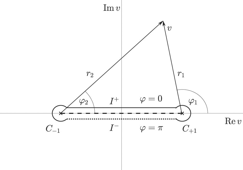
The same procedure can be done very elegantly by continuing integral (15) into the complex domain, see figure A2. The variable transformation x = sin(u), used to go from (15) to (16), introduces multi-valuedness that needs to be resolved by an appropriate definition of the integration contour. The factor $1/\sqrt{1-{v}^{2}}$ in (16b) is multi-valued and has branch points at v = ±1. We introduce a branch cut between −1 and 1 to make the function single-valued. Points v infinitesimally above and below the branch cut are denoted by v^± = v ± iɛ.

Zoom In Zoom Out Reset image size

The branch cut is defined by setting v + 1 = r₂ exp(iφ₂) and v − 1 = r₁ exp(iφ₁) with 0 ⩽ φ₁, φ₂ < 2π which results in $\sqrt{1-{v}^{2}}=\sqrt{{r}_{1}{r}_{2}}\,\mathrm{exp}(i\varphi )$ with φ = (φ₁ + φ₂ − π)/2. As φ₁ ≈ π, π and φ₂ = 0, 2π we find φ = 0, π for v on I⁺ and I⁻, respectively. As a result, ${\mathrm{lim}}_{\varepsilon \to 0}\sqrt{1-{v}_{\pm }^{2}}\to \pm \sqrt{1-{v}^{2}}$. This agrees with the ± difference between the square root evaluated on I⁺ and I⁻, respectively, obtained before in the real domain. As a result, we find that the ± difference can be realized by choosing I⁺ and I⁻ to be located above and below the real axis, respectively. We connect I⁺ and I⁻ by infinitesimal circles (C_±1) around v = ±1 which yields the dog bone contour in figure A2. As such, the requirement of a single valued integrand has defined the integration contour of the integral

$$\begin{align}\hfill \begin{aligned}\hfill L(\mathbf{P})& =\frac{1}{2\pi }\oint \!{V}_{0}\!\left(\!\mathbf{P}+\frac{\mathbf{F}}{\omega }u\!\right){e}^{i\frac{S(u)}{\omega }}\!du\hfill \\ \hfill \frac{S(u)}{\omega }& ={\int }_{0}^{u}\frac{(n-{c}_{2})+{c}_{1}v+2{c}_{2}{v}^{2}}{\sqrt{1-{v}^{2}}}\,dv\hfill \end{aligned}\end{align} \tag{ A.3 }$$

in the complex plane. The integral defining S(u) on the real axis is

$$\begin{align}\hfill & {\int }_{0}^{u}\frac{2{c}_{2}{v}^{2}+{c}_{1}v+(n-{c}_{2})}{\sqrt{1-{v}^{2}}}\,dv\hfill \\ \hfill & \hspace{25.0pt}=n\,{\mathrm{sin}}^{-1}(u)-({c}_{1}+{c}_{2}u)\sqrt{1-{u}^{2}}.\hfill \end{align} \tag{ A.4 }$$

What remains to be done is to evaluate integral (A.4) on the complex integration contour and to show that the result agrees with the integrals in (A.2). The integral along the dogbone contour consists of an integral along ${I}_{a}^{+}$ from 0⁺ → 1⁺, a circular integral along C₊₁, an integral along I⁻ from 1⁻ → −1⁻, another circular integral along C₋₁, and finally an integral ${I}_{b}^{+}$ from −1⁺ → 0⁺. The two circular integrals drop out, as they scale $\propto {\mathrm{lim}}_{\varepsilon \to 0}\sqrt{(}\varepsilon )=0$. We denote ${S}_{{I}_{a}^{+}}({u}^{+})$, ${S}_{{I}^{-}}({u}^{-})$, and ${S}_{{I}_{b}^{+}}({u}^{+})$, as the integrals for which u lies in the intervals of ${I}_{a}^{+}$, I⁻, ${I}_{b}^{+}$, respectively. With the help of (A.4) we obtain

$$\begin{align}\hfill \frac{{S}_{{I}_{a}^{+}}({u}^{+})}{\omega }& ={\int }_{0}^{{u}^{+}}\frac{(n-{c}_{2})+{c}_{1}v+2{c}_{2}{v}^{2}}{\sqrt{1-{v}^{2}}}\,dv\hfill \\ \hfill & =n\,{\mathrm{sin}}^{-1}(u)-({c}_{1}+{c}_{2}u)\sqrt{1-{u}^{2}},\hfill \end{align} \tag{ A.5a }$$

$$\begin{align}\hfill \frac{{S}_{{I}^{-}}({u}^{-})}{\omega }& =\frac{{S}_{{I}_{a}^{+}}({1}^{+})}{\omega }+{\int }_{{1}^{-}}^{{u}^{-}}\frac{(n-{c}_{2})+{c}_{1}v+2{c}_{2}{v}^{2}}{-\sqrt{1-{v}^{2}}}\,dv\hfill \\ \hfill & =n\left(\pi -{\mathrm{sin}}^{-1}(u)\right)+\,({c}_{1}+{c}_{2}u)\sqrt{1-{u}^{2}},\hfill \end{align} \tag{ A.5b }$$

where ${S}_{{I}_{a}^{+}}({1}^{+})/\omega =n\pi /2$, and

$$\begin{align}\hfill \frac{{S}_{{I}_{b}^{+}}({u}^{+})}{\omega }& =\frac{{S}_{{I}^{-}}(-{1}^{-})}{\omega }+{\int }_{-{1}^{+}}^{{u}^{+}}\frac{(n-{c}_{2})+{c}_{1}v+2{c}_{2}{v}^{2}}{\sqrt{1-{v}^{2}}}\,dv\hfill \\ \hfill & =n\left(2\pi +{\mathrm{sin}}^{-1}(u)\right)-\left({c}_{1}+{c}_{2}u\right)\sqrt{1-{u}^{2}}\hfill \end{align} \tag{ A.5c }$$

with ${S}_{{I}^{-}}(-{1}^{-})/\omega =3n\pi /2$. The classical actions in all three segments agree with the phase terms in (A.2) which shows that the treatments in the real and complex domains are consistent.